
Fatigue Load Modeling of Floating Wind Turbines Based on Vine Copula Theory and Machine Learning

 , and
, and
Abstract
:1. Introduction
- (1)
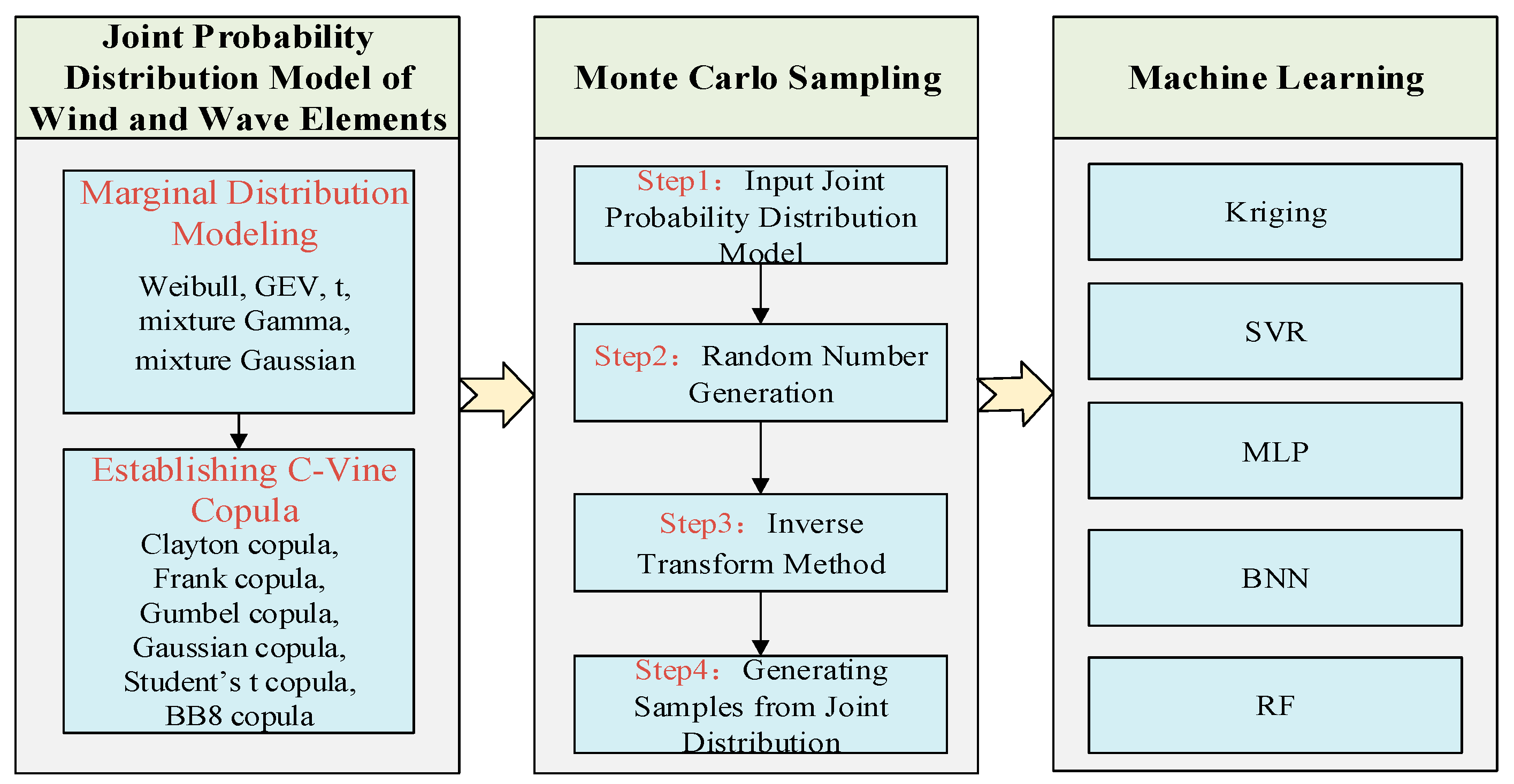
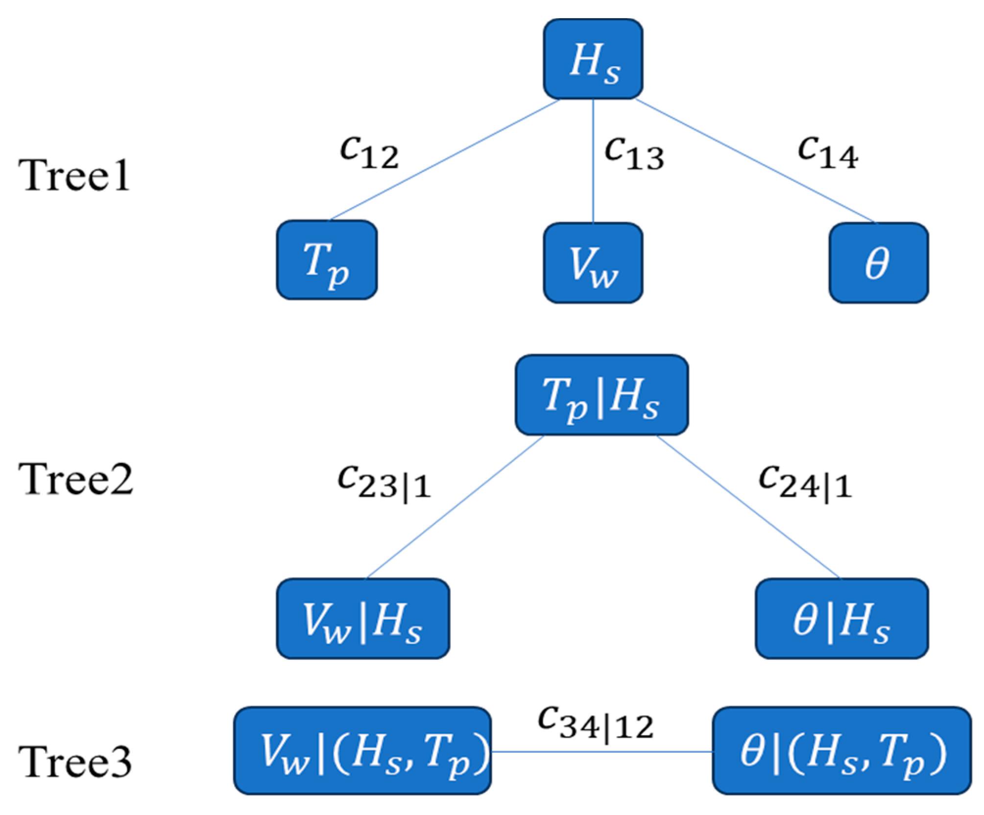
- Establishing a joint probability distribution model of wind and wave elements based on Vine copula theory: Using long-term meteorological and oceanographic data from marine sites, selecting appropriate wind and wave elements as variables, and constructing a long-term joint probability distribution model using the C-Vine copula model to capture dependencies among multivariate wind and wave environments;
- (2)
- Developing a data-driven load model using machine learning: Using five machine learning algorithms (Kriging, MLP, SVR, BNN, and RF) to build data-driven models. Input variables include easily measurable data such as wind and wave environment variables (wind speed, wave height, wave period, wind direction) and wind turbine motion state variables (yaw, rotor speed, pitch angle), selected through correlation analysis. Output variables are DEL for two key components of the wind turbine: blade root and tower base;
- (3)
- Validating the proposed method with real marine site data: Using measured wind and wave data from the Lianyungang marine observation station in the East China Sea, conducting OpenFAST simulation experiments and actual data verification to evaluate the performance and accuracy of the proposed method.
2. Methodologies
2.1. Joint Probability Distribution Model of Wind and Wave Elements
2.1.1. Marginal Distribution Modeling
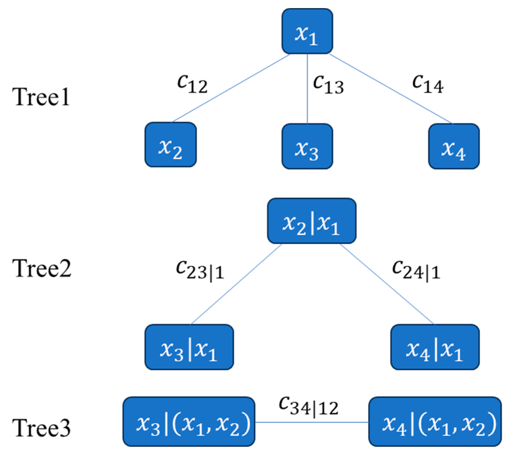
2.1.2. Joint Distribution Modeling
2.2. Monte Carlo Sampling Method
2.3. FAST Simulation and Fatigue Load Estimation Method
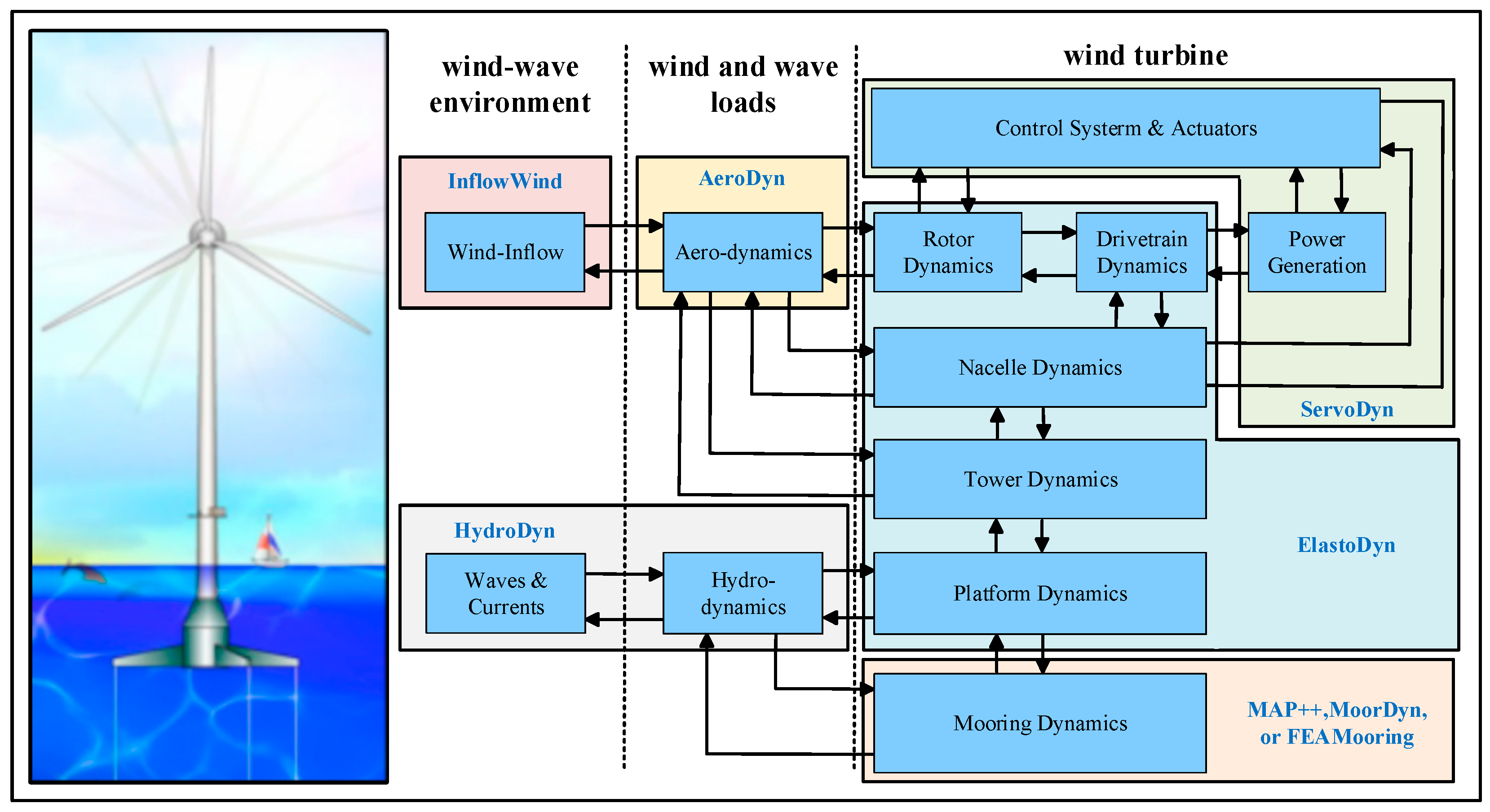
2.3.1. OpenFAST Simulation Method
2.3.2. Fatigue Load Assessment Method
2.4. Machine Learning-Based Fatigue Load Modeling Method
| Algorithm 1 Damage Equivalent Load (DEL) Prediction and Model Selection |
| Input: Environment variables: wind_speed, wave_height, wave_period, wind_direction Turbine state variables: yaw_angle, rotor_speed, blade_pitch DEL: RootMxb1, RootMyb1, RootMzb1, TwrBsMxt, TwrBsMyt, TwrBsMzt Output: Best model among Kriging, MLP, SVR, BNN, RF based on overall error 1. Correlation Analysis: Compute correlation coefficients between: - wind_speed, wave_height, wave_period, wind_direction - yaw_angle, rotor_speed, blade_pitch and - RootMxb1, RootMyb1, RootMzb1, TwrBsMxt, TwrBsMyt, TwrBsMzt 2. Select Input Variables: Select top four variables with highest absolute correlation coefficients with DEL: - selected_input_variables = [var1, var2, var3, var4] 3. Machine Learning Models Training and Prediction: Initialize models: Kriging, MLP, SVR, BNN, RF for each model in [Kriging, MLP, SVR, BNN, RF]: Train model using selected_input_variables to predict DEL values: - model.train(X_train[selected_input_variables], y_train[DEL]) Predict DEL values for test dataset: - predicted_DEL = model.predict(X_test[selected_input_variables]) Calculate overall error (e.g., MSE) for the model: - overall_error = calculate_error(predicted_DEL, y_test[DEL]) Store model and its overall error 4. Select Best Model: Identify model with minimum overall error: - best_model = model with minimum overall_error 5. Output Results: Print or store predicted DEL values and evaluation metrics for best_model. End Algorithm |
2.5. Framework for Fatigue Load Modeling of Floating Wind Turbines
- (1)
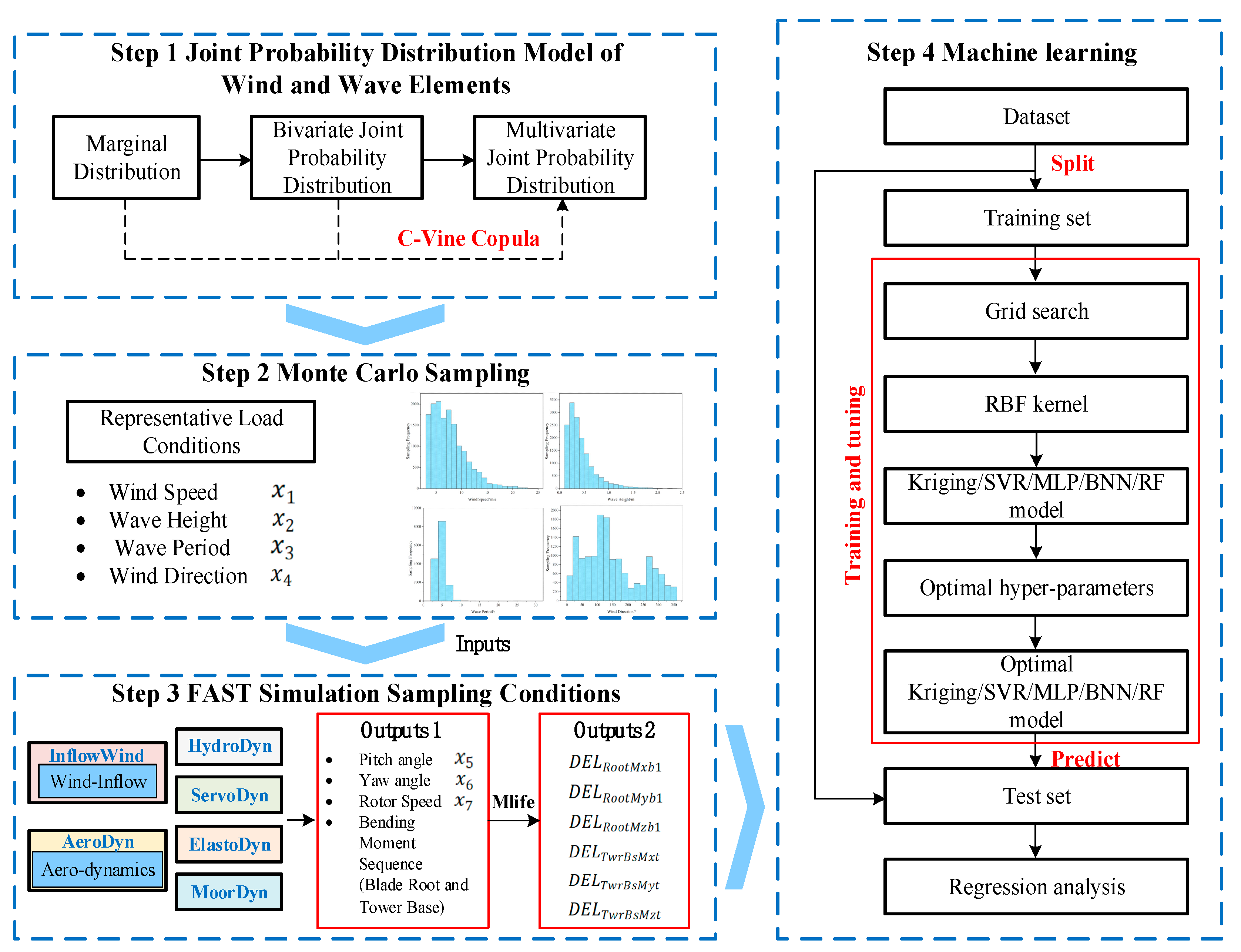
- Establishment of joint probability distribution models for wind and wave factors: Marginal distribution model parameters for each wind and wave factor are determined using maximum likelihood estimation. The goodness of fit is evaluated using AIC, BIC, and RMSE criteria to establish marginal distributions of wind and wave factors. Subsequently, parameters of the two-dimensional copula function are estimated within a Bayesian framework using a Gaussian likelihood function based on residuals, with model selection based on AIC for optimal copula function determination. Finally, the C-Vine copula theory is employed to establish a joint probability distribution model for the four-dimensional random variables: wind speed, wave height, wave period, and wind direction;
- (2)
- Monte Carlo sampling for representative sample conditions: Following construction of the joint PDF of ocean environmental variables, Monte Carlo sampling is employed to obtain representative sample conditions of wind speed (), wave height (), wave period (), and wind direction () as input conditions for subsequent simulation modeling;
- (3)
- FAST simulation under-sampled conditions: To establish a data-driven model for fatigue load data at critical components such as blade roots and tower bases of floating wind turbines, a substantial volume of effective data is required to build the database. Post identification of representative load conditions, OpenFAST is utilized to model fatigue loads for all sampled conditions;
- (4)
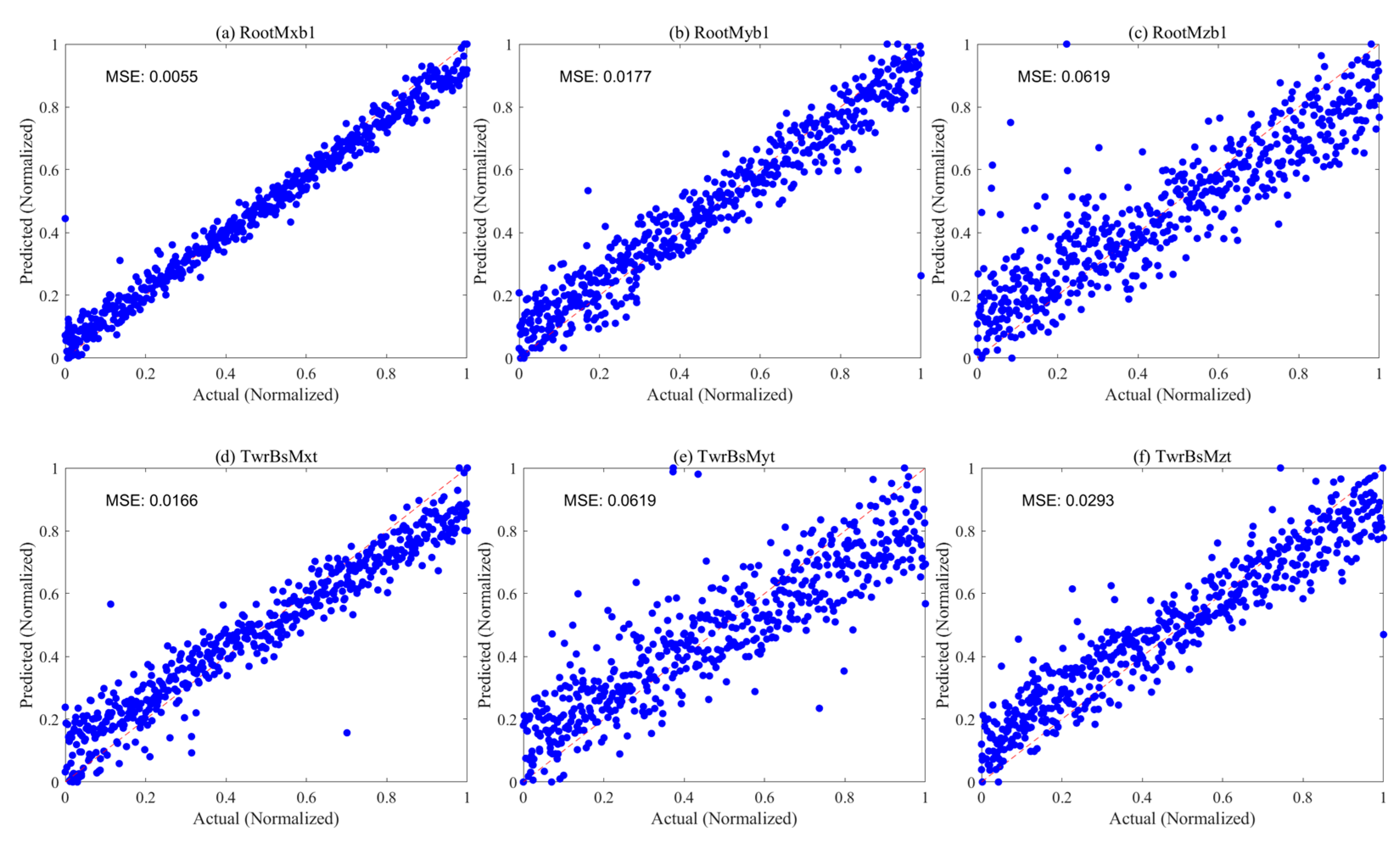
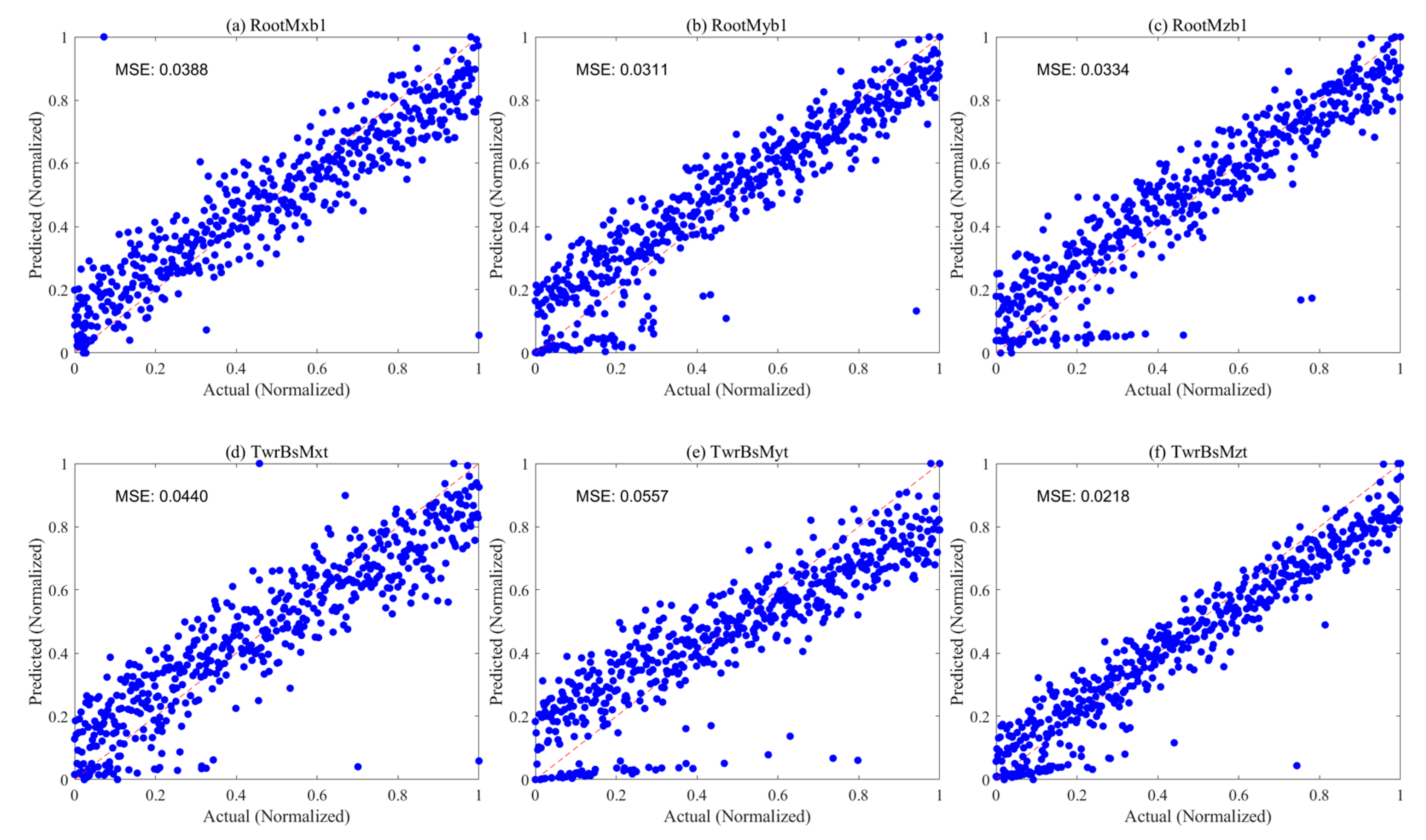
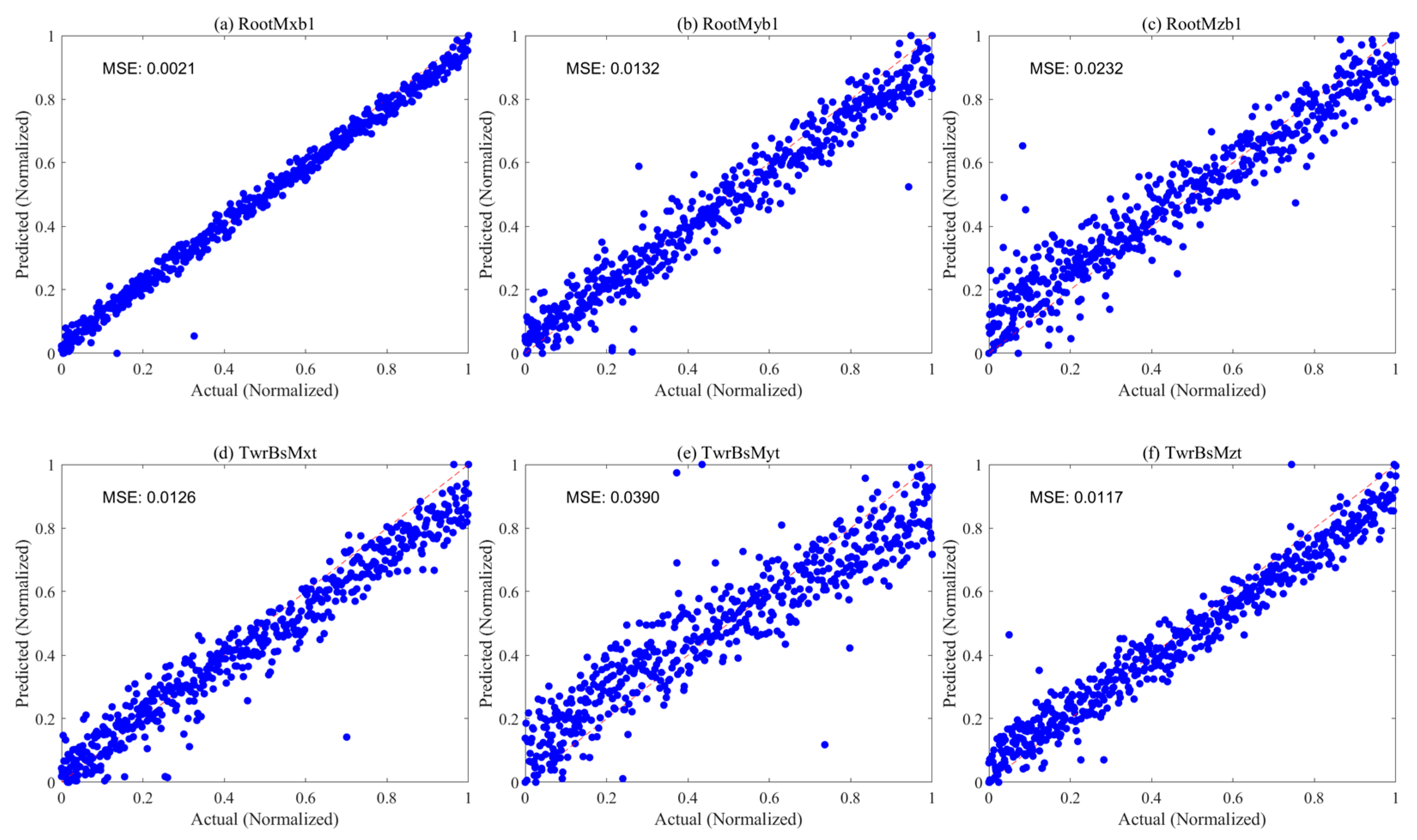
- Machine learning-based damage equivalent load modeling: Machine learning techniques are employed to construct fatigue load models. Model inputs include environmental variables (wind speed, wave height, wave period, wind direction) and operational state variables (rotor speed, yaw angle, blade pitch angle). Outputs consist of damage equivalent loads for six key moments at blade roots (RootMxb1, RootMyb1, and RootMzb1) and tower bases (TwrBsMxt, TwrBsMyt, and TwrBsMzt).
3. Case Study
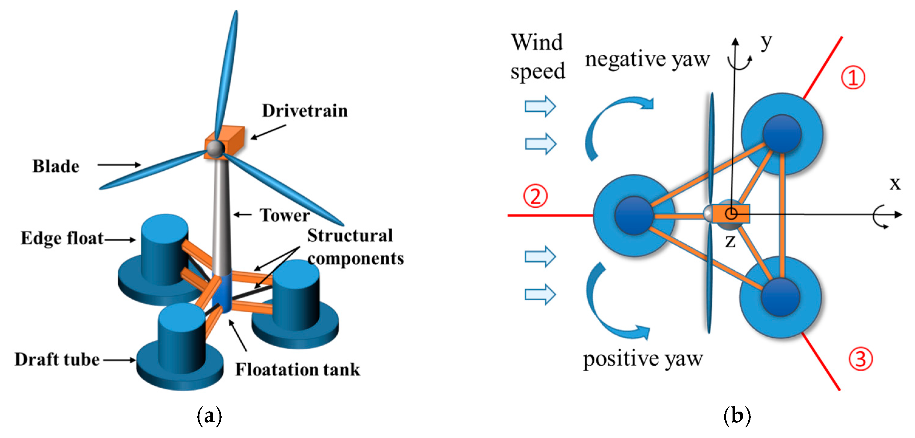
3.1. Study Object
3.2. Analysis of Joint Probability Distribution Modeling Results of Wind and Wave Factors
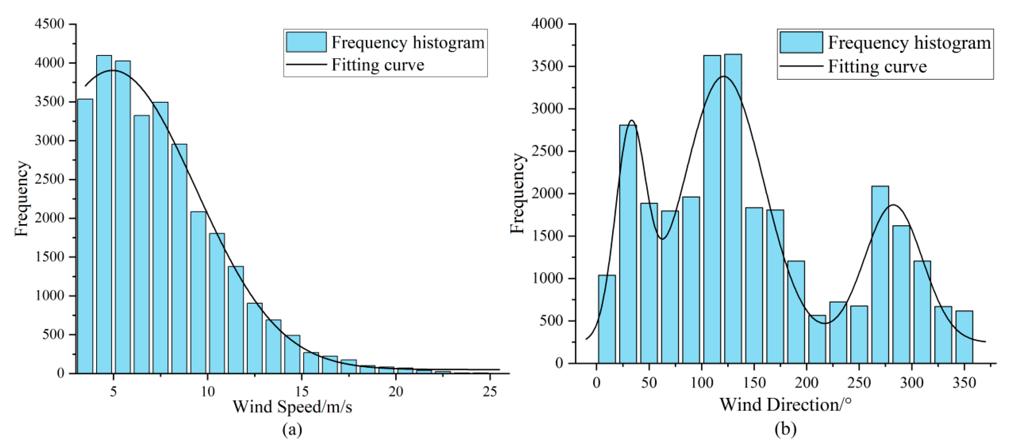
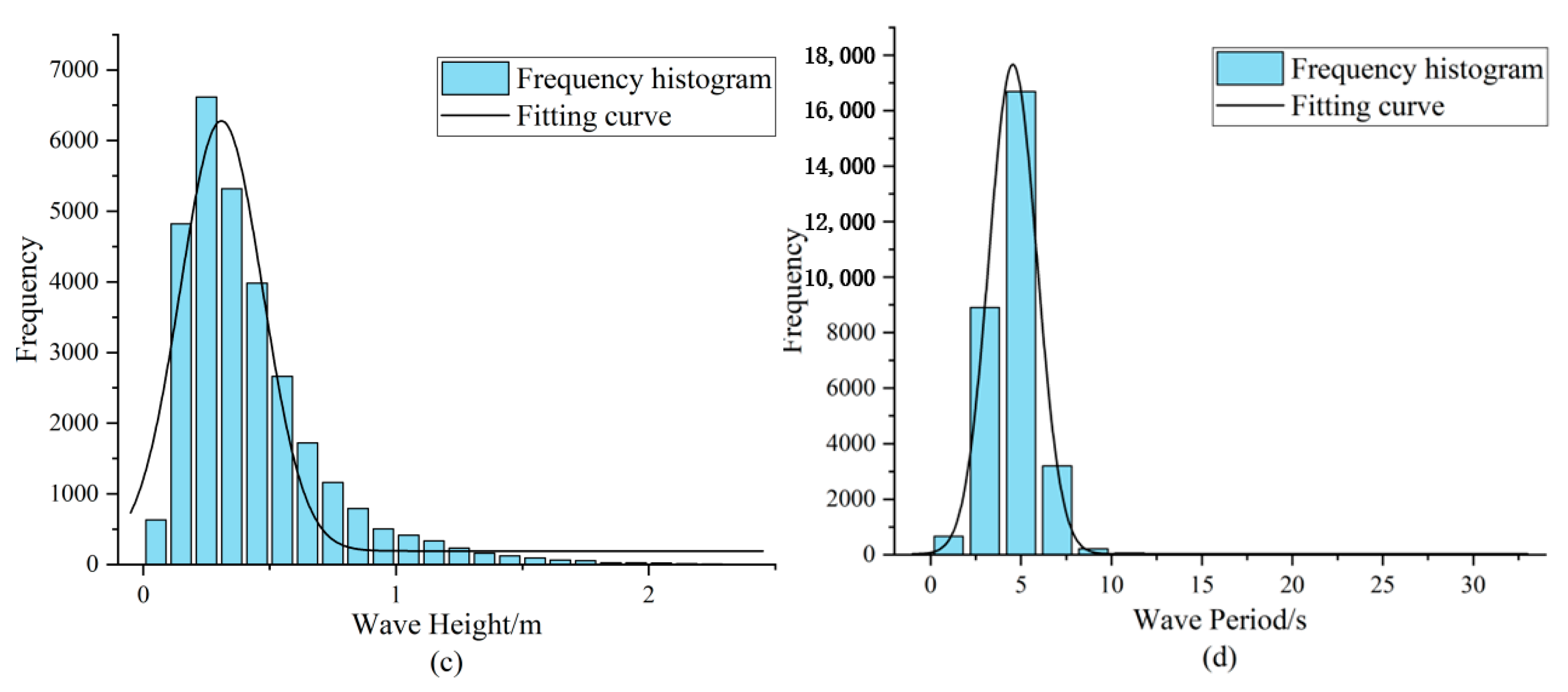
3.2.1. Data Description
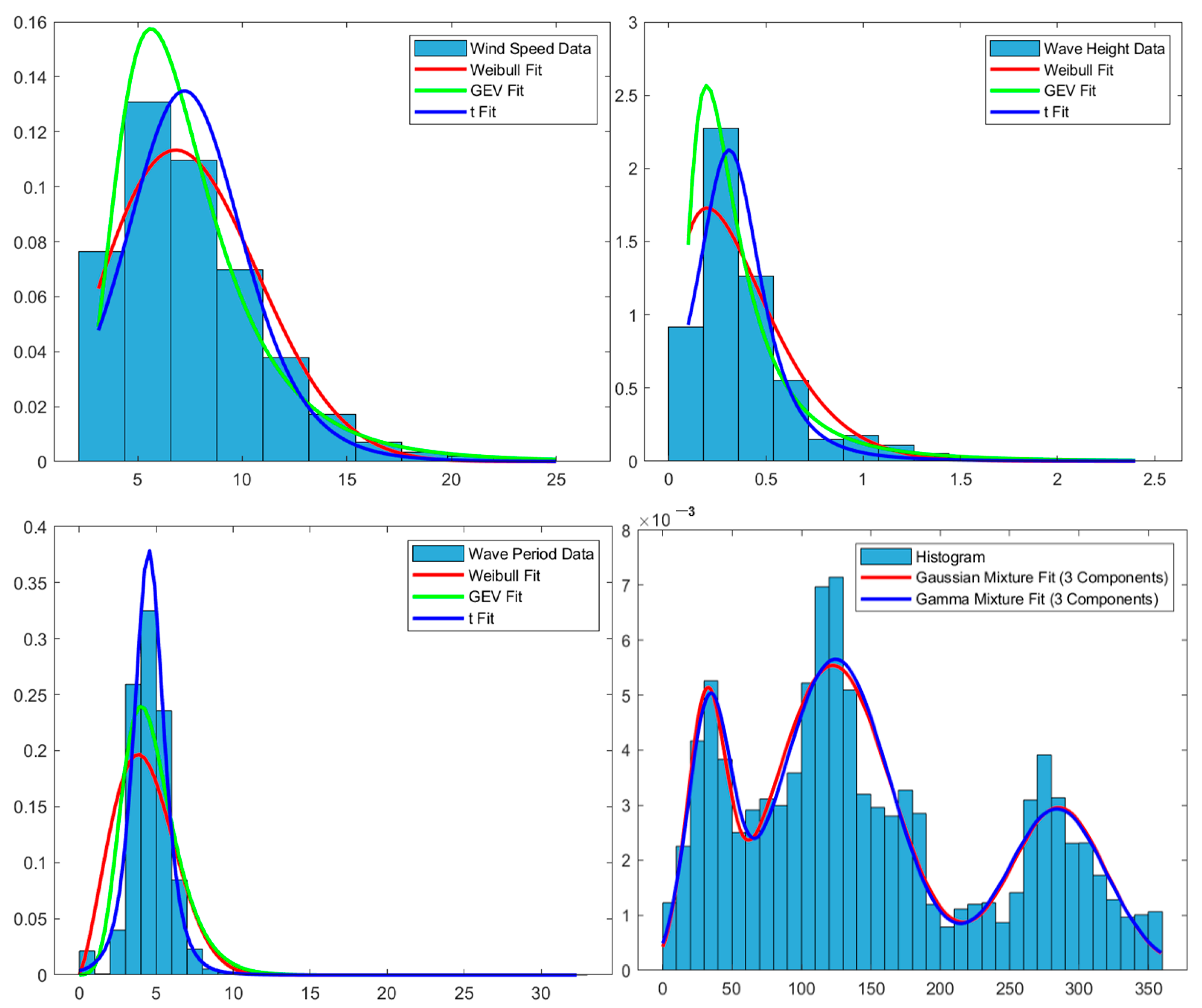
3.2.2. Results of Marginal Distribution Modeling
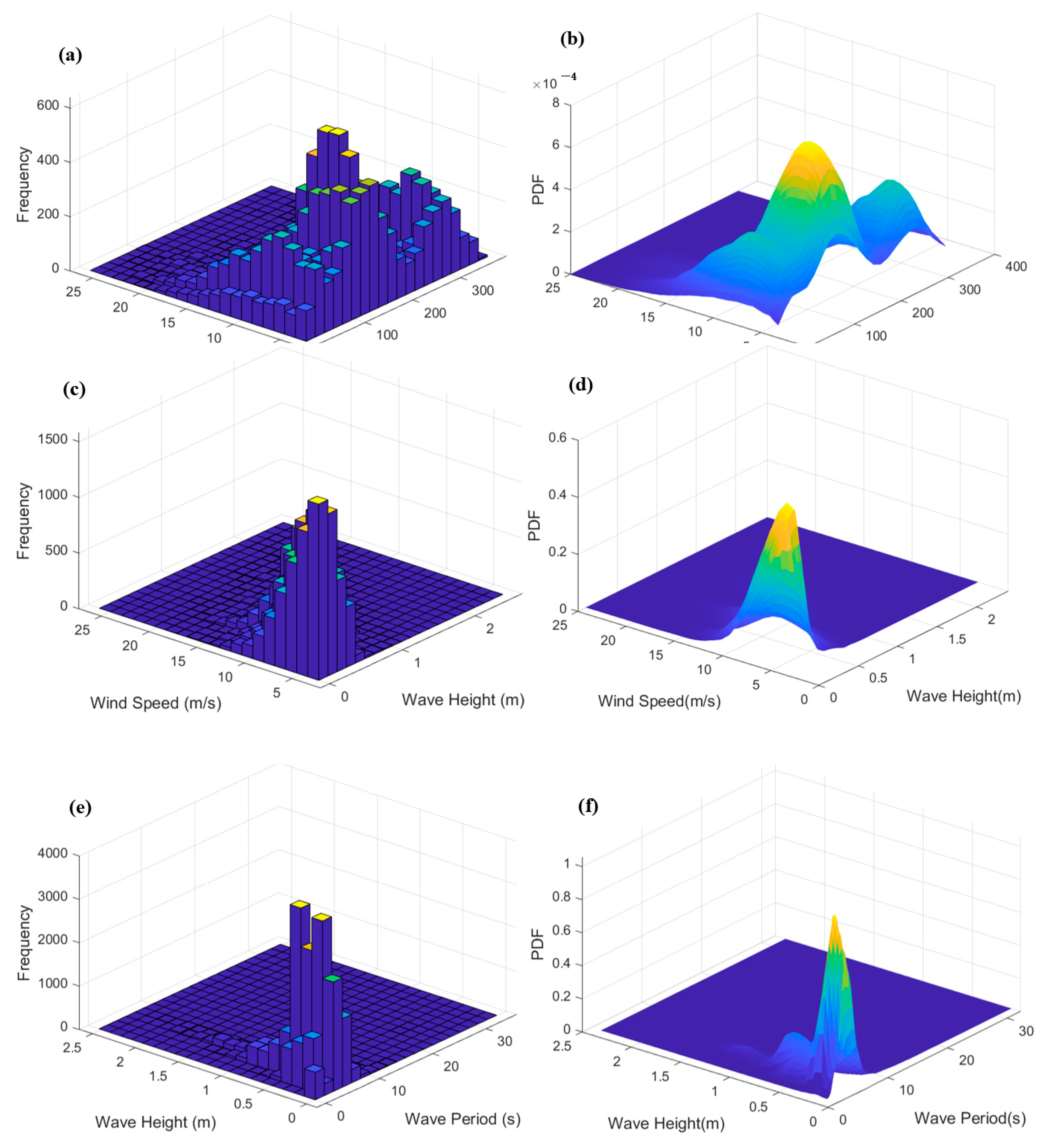
3.2.3. Joint Distribution Modeling Results
3.3. Analysis of Fatigue Load Modeling Based on Machine Learning
3.3.1. Simulation Parameter Settings and Correlation Analysis
3.3.2. Modeling Results of Data-Driven Models
4. Conclusions
- (1)
- Detailed analysis of measured data from the Lianyungang marine site in the East China Sea reveals that wind speed, wave height, and wave period exhibit unimodal distribution characteristics suitable for fitting with common unimodal distribution models, whereas wind direction shows multimodal distribution characteristics requiring a mixture model for fitting. Specifically, the optimal fitting distributions are the Weibull distribution for wind speed, Generalized Extreme Value (GEV) distribution for wave height, t-distribution with scale parameter for wave period, and mixed Gaussian distribution for wind direction. The Root Mean Square Error for fitting these four variables is all less than 0.01, indicating the good performance of the selected optimal marginal probability distribution models in fitting;
- (2)
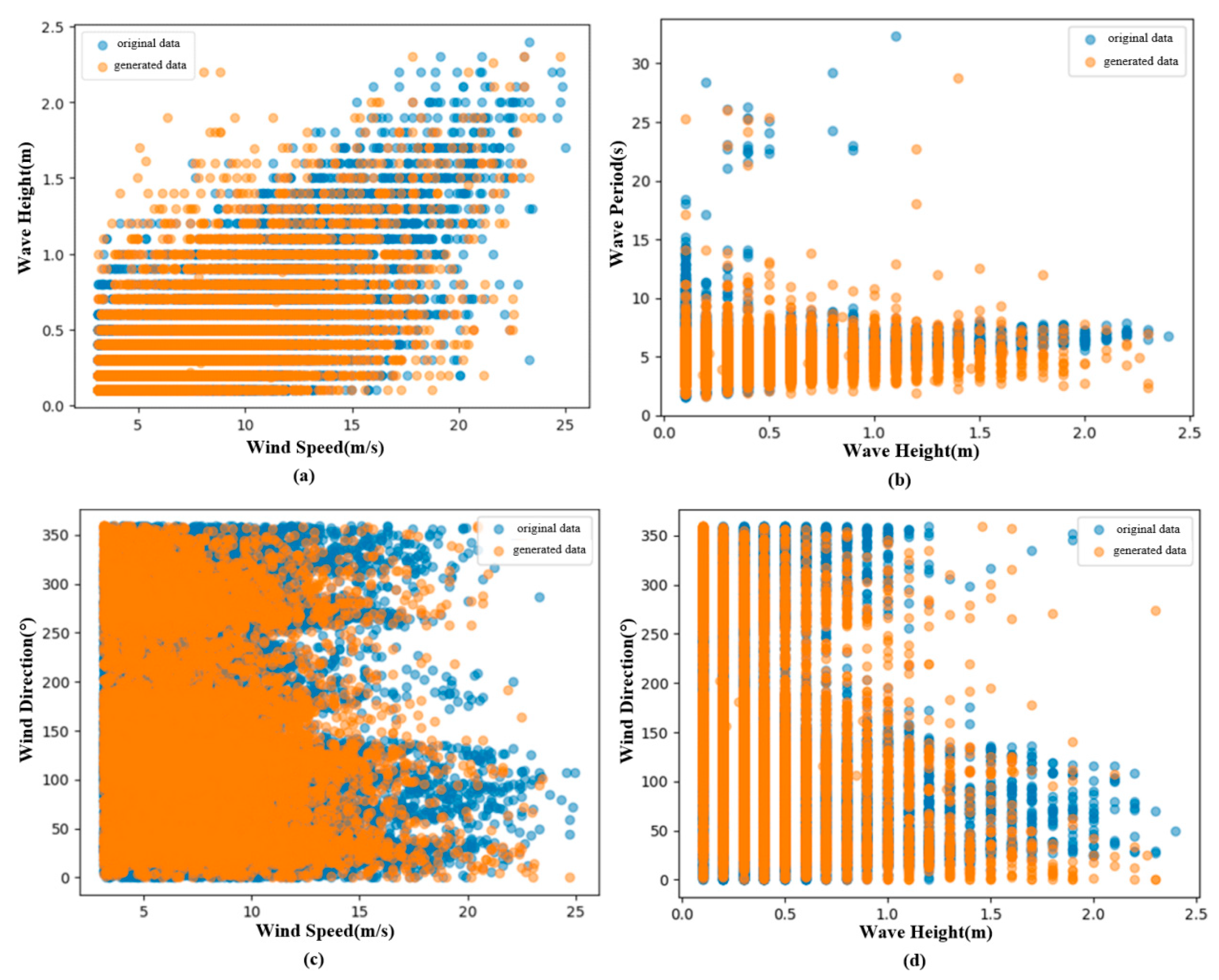
- The established C-Vine copula model effectively characterizes the joint probability distribution between the four-dimensional random variables of wind speed, wave height, wave period, and wind direction. Specifically, comparing the probability dependency characteristics of model-generated samples with original data reveals a high degree of consistency between the two. Additionally, the Kolmogorov–Smirnov (K-S) test statistic of 0.0025 indicates that the distribution of generated samples is nearly identical to that of the original data. The K-S test p-value of 0.9917 further confirms that there is no significant difference between generated samples and original data. These results demonstrate the reliability and effectiveness of the model in simulating environmental variables;
- (3)
- For predicting fatigue loads of floating wind turbine root and tower base moments, the RF model demonstrates superior prediction performance and generalization ability, achieving outstanding results with a minimum MSE of only 0.0021 for predicting six DEL values. While the Kriging model approaches the accuracy of the RF model on some variables, it exhibits slight degradation in high-dimensional spaces. In contrast, MLP and BNN models show higher prediction errors, especially the BNN model with an MSE exceeding 0.3 in some predictions, indicating limited prediction accuracy. Therefore, it is recommended that the RF model be selected as the preferred method for establishing DEL prediction models for root and tower base moments in practical applications, ensuring the accuracy and reliability of prediction results.
Author Contributions
Funding
Institutional Review Board Statement
Informed Consent Statement
Data Availability Statement
Conflicts of Interest
Abbreviations
| FOWT | Floating Offshore Wind Turbine |
| C-Vine copula | Canonical Vine copula |
| CDF | Cumulative Distribution Function |
| Probability Density Function | |
| GEV | Generalized Extreme Value distribution |
| AIC | Akaike Information Criterion |
| BIC | Bayesian Information Criterion |
| RMSE | Evaluate the goodness of fit of different probability distribution models |
| The expression for the BB8 copula | |
| Evaluate the goodness of fit of the selected copula functions | |
| Kriging | Geostatistical Kriging |
| MLP | Multilayer Perceptron |
| SVR | Support Vector Regression |
| BNN | Bayesian Neural Network |
| RF | Random Forest |
| DEL | Damage Equivalent Load |
| var1, var2, var3, var4 | Marine environmental variables 1, 2, 3, and 4, respectively |
| RootMxb1 | Edgewise bending moment at the blade root |
| RootMyb1 | Flapwise bending moment at the blade root |
| RootMzb1 | The z-directional bending moment at the blade root |
| TwrBsMxt | Side-side (or roll) bending moment at the tower base |
| TwrBsMyt | Fore-aft (or pitch) bending moment at the tower base |
| TwrBsMzt | The z-directional bending moment at the tower base |
| MSE/RMSE/ | Evaluate machine learning model errors |
References
- Global Wind Energy Council. Global Wind Report 2023. Available online: https://gwec.net/globalwindreport2023/ (accessed on 1 November 2023).
- Global Wind Energy Council. Global Wind Report 2024. Available online: https://gwec.net/global-wind-report-2024/ (accessed on 20 June 2024).
- Robertson, B.; Dunkle, G.; Gadasi, J.; Garcia-Medina, G.; Yang, Z. Holistic marine energy resource assessments: A wave and offshore wind perspective of metocean conditions. Renew. Energy 2021, 170, 286–301. [Google Scholar] [CrossRef]
- Offshore Wind Energy (OWE). Technology of OWE. 2009. Available online: http://www.offshorewindenergy.org/ (accessed on 26 July 2024).
- Alkhabbaz, A.; Hamza, H.; Daabo, A.M.; Yang, H.S.; Yoon, M.; Koprulu, A.; Lee, Y.H. The aero-hydrodynamic interference impact on the NREL 5-MW floating wind turbine experiencing surge motion. Ocean Eng. 2024, 295, 116970. [Google Scholar] [CrossRef]
- Edirisinghe, D.S.; Yang, H.S.; Gunawardane, S.; Alkhabbaz, A.; Tongphong, W.; Yoon, M.; Lee, Y.H. Numerical and experimental investigation on water vortex power plant to recover the energy from industrial wastewater. Renew. Energy 2023, 204, 617–634. [Google Scholar] [CrossRef]
- Guo, Y.; Wang, H.; Lian, J. Review of integrated installation technologies for offshore wind turbines: Current progress and future development trends. Energy Convers. Manag. 2022, 255, 115319. [Google Scholar] [CrossRef]
- Bitner-Gregersen, E.M.; Dong, S.; Fu, T.; Ma, N.; Maisondieu, C.; Miyake, R.; Rychlik, I. Sea state conditions for marine structures’ analysis and model tests. Ocean Eng. 2016, 119, 309–322. [Google Scholar] [CrossRef]
- Czado, C.; Nagler, T. Vine copula based modeling. Annu. Rev. Stat. Its Appl. 2022, 9, 453–477. [Google Scholar] [CrossRef]
- Li, X.; Zhang, W. Long-term assessment of a floating offshore wind turbine under environmental conditions with multivariate dependence structures. Renew. Energy 2020, 147, 764–775. [Google Scholar] [CrossRef]
- Zhao, Y.; Dong, S. Multivariate probability analysis of wind-wave actions on offshore wind turbine via copula-based analysis. Ocean Eng. 2023, 288, 116071. [Google Scholar] [CrossRef]
- Det Norske Veritas. Environmental Conditions and Environmental Loads; Det Norske Veritas: Oslo, Norway, 2000. [Google Scholar]
- Sutherland, H.J. On the Fatigue Analysis of Wind Turbines. 1999. Available online: https://www.osti.gov/biblio/9460 (accessed on 30 November 2023).
- Offshore Standard DNV-OS-J101; Design of Offshore Wind Turbine Structure. Det Norske Veritas: Oslo, Norway, 2004.
- Yang, J.; Zheng, S.; Song, D.; Su, M.; Yang, X.; Joo, Y.H. Data-driven modeling for fatigue loads of large-scale wind turbines under active power regulation. Wind Energy 2021, 24, 558–572. [Google Scholar] [CrossRef]
- He, R.; Yang, H.; Lu, L. Optimal yaw strategy and fatigue analysis of wind turbines under the combined effects of wake and yaw control. Appl. Energy 2023, 337, 120878. [Google Scholar] [CrossRef]
- Woo, S.; Park, J.; Park, J. Predicting wind turbine power and load outputs by multi-task convolutional LSTM model. In Proceedings of the 2018 IEEE Power & Energy Society General Meeting (PESGM), Portland, OR, USA, 5–10 August 2018; pp. 1–5. [Google Scholar]
- Yao, Q.; Ma, B.; Zhao, T.; Hu, Y.; Fang, F. Optimized active power dispatching of wind farms considering data-driven fatigue load suppression. IEEE Trans. Sustain. Energy 2022, 14, 371–380. [Google Scholar] [CrossRef]
- Sun, J.; Chen, Z.; Yu, H.; Gao, S.; Wang, B.; Ying, Y.; Sun, Y.; Qian, P.; Zhang, D.; Si, Y. Quantitative evaluation of yaw-misalignment and aerodynamic wake induced fatigue loads of offshore Wind turbines. Renew. Energy 2022, 199, 71–86. [Google Scholar] [CrossRef]
- Yin, X.; Lei, M. Jointly improving energy efficiency and smoothing power oscillations of integrated offshore wind and photovoltaic power: A deep reinforcement learning approach. Prot. Control Mod. Power Syst. 2023, 8, 1–11. [Google Scholar] [CrossRef]
- Wang, Y.; Gu, J.; Yuan, L. Distribution network state estimation based on attention-enhanced recurrent neural network pseudo-measurement modeling. Prot. Control Mod. Power Syst. 2023, 8, 1–16. [Google Scholar] [CrossRef]
- Ahsan, F.; Dana, N.H.; Sarker, S.K.; Li, L.; Muyeen, S.M.; Ali, M.F.; Tasneem, Z.; Hasan, M.M.; Abhi, S.H.; Islam, M.R.; et al. Data-driven next-generation smart grid towards sustainable energy evolution: Techniques and technology review. Prot. Control Mod. Power Syst. 2023, 8, 1–42. [Google Scholar] [CrossRef]
- Ghalandari, M.; Mukhtar, A.; Yasir, A.S.H.M.; Alkhabbaz, A.; Alviz-Meza, A.; Cárdenas-Escrocia, Y.; Le, B.N. Thermal conductivity improvement in a green building with Nano insulations using machine learning methods. Energy Rep. 2023, 9, 4781–4788. [Google Scholar] [CrossRef]
- Song, D.; Shen, G.; Huang, C.; Huang, Q.; Yang, J.; Dong, M.; Joo, Y.H.; Duić, N. Review on the application of artificial intelligence methods in the control and design of offshore wind power systems. J. Mar. Sci. Eng. 2024, 12, 424. [Google Scholar] [CrossRef]
- Song, D.; Tan, X.; Huang, Q.; Wang, L.; Dong, M.; Yang, J.; Evgeny, S. Review of AI-based wind prediction within recent three years: 2021–2023. Energies 2024, 17, 1270. [Google Scholar] [CrossRef]
- Yang, H.S.; Alkhabbaz, A.; Tongphong, W.; Lee, Y.H. Cross-comparison analysis of environmental load components in extreme conditions for pontoon-connected semi-submersible FOWT using CFD and potential-based tools. Ocean Eng. 2024, 304, 117248. [Google Scholar] [CrossRef]
- Yang, H.S.; Tongphong, W.; Ali, A.; Lee, Y.H. Comparison of different fidelity hydrodynamic-aerodynamic coupled simulation code on the 10 MW semi-submersible type floating offshore wind turbine. Ocean Eng. 2023, 281, 114736. [Google Scholar] [CrossRef]
- Aas, K.; Czado, C.; Frigessi, A.; Bakken, H. Pair-copula constructions of multiple dependence. Insur. Math. Econ. 2009, 44, 182–198. [Google Scholar] [CrossRef]
- Murthy, D.N.P.; Xie, M.; Jiang, R. Weibull Models; John Wiley & Sons: Hoboken, NJ, USA, 2004. [Google Scholar]
- Bali, T.G. The generalized extreme value distribution. Econ. Lett. 2003, 79, 423–427. [Google Scholar] [CrossRef]
- Tate, R.F. Unbiased estimation: Functions of location and scale parameters. Ann. Math. Stat. 1959, 30, 341–366. [Google Scholar] [CrossRef]
- Thom, H.C.S. Approximate convolution of the gamma and mixed gamma distributions. Mon. Weather Rev. 1968, 96, 883–886. [Google Scholar] [CrossRef]
- Murray, J.S.; Dunson, D.B.; Carin, L.; Lucas, J.E. Bayesian Gaussian copula factor models for mixed data. J. Am. Stat. Assoc. 2013, 108, 656–665. [Google Scholar] [CrossRef] [PubMed]
- Nelsen, R.B. An Introduction to Copulas; Springer: New York, NY, USA, 2006. [Google Scholar]
- Ehsan, M.A.; Shahirinia, A.; Gill, J.; Zhang, N. Dependent wind speed models: Copula approach. In Proceedings of the 2020 IEEE Electric Power and Energy Conference (EPEC), Edmonton, AB, Canada, 9–10 November 2020; pp. 1–6. [Google Scholar]
- Bretthorst, G.L. An introduction to parameter estimation using bayesian probability theory. In Maximum Entropy and Bayesian Methods; Springer: Dordrecht, The Netherlands, 1990; pp. 53–79. [Google Scholar]
- Schoups, G.; Vrugt, J.A. A formal likelihood function for parameter and predictive inference of hydrologic models with correlated, heteroscedastic, and non-Gaussian errors. Water Resour. Res. 2010, 46, W10531. [Google Scholar] [CrossRef]
- Kvittem, M.I.; Moan, T. Time domain analysis procedures for fatigue assessment of a semi-submersible wind turbine. Mar. Struct. 2015, 40, 38–59. [Google Scholar] [CrossRef]
- Chian, C.Y.; Zhao, Y.Q.; Lin, T.Y.; Nelson, B.; Huang, H.H. Comparative study of time-domain fatigue assessments for an offshore wind turbine jacket substructure by using conventional grid-based and monte carlo sampling methods. Energies 2018, 11, 3112. [Google Scholar] [CrossRef]
- Openfast v3.1.0. 2022. Available online: https://github.com/OpenFAST/openfast (accessed on 20 May 2022).
- Golparvar, B.; Papadopoulos, P.; Ezzat, A.A.; Wang, R.Q. A surrogate-model-based approach for estimating the first and second-order moments of offshore wind power. Appl. Energy 2021, 299, 117286. [Google Scholar] [CrossRef]
- Hayman, G.J. MLife Theory Manual for Version 1.00; National Renewable Energy Laboratory: Golden, CO, USA, 2012.
- Yuan, Y.; Tang, J. Adaptive pitch control of wind turbine for load mitigation under structural uncertainties. Renew. Energy 2017, 105, 483–494. [Google Scholar] [CrossRef]
- Li, H.; Hu, Z.; Wang, J.; Meng, X. Short-term fatigue analysis for tower base of a spar-type wind turbine under stochastic wind-wave loads. Int. J. Nav. Archit. Ocean Eng. 2018, 10, 9–20. [Google Scholar] [CrossRef]
- Manwell, J.F.; McGowan, J.G.; Rogers, A.L. Wind Energy Explained: Theory, Design and Application; John Wiley & Sons: Hoboken, NJ, USA, 2010. [Google Scholar]
- Cressie, N. The origins of kriging. Math. Geol. 1990, 22, 239–252. [Google Scholar] [CrossRef]
- Pinkus, A. Approximation theory of the MLP model in neural networks. Acta Numer. 1999, 8, 143–195. [Google Scholar] [CrossRef]
- Terrault, N.A.; Hassanein, T.I. Management of the patient with SVR. J. Hepatol. 2016, 65, S120–S129. [Google Scholar] [CrossRef]
- Lampinen, J.; Vehtari, A. Bayesian approach for neural networks—Review and case studies. Neural Netw. 2001, 14, 257–274. [Google Scholar] [CrossRef]
- Rigatti, S.J. Random forest. J. Insur. Med. 2017, 47, 31–39. [Google Scholar] [CrossRef]
- Jonkman, J.; Butterfield, S.; Musial, W.; Scott, G. Definition of a 5-MW Reference wind Turbine for Offshore System Development; National Renewable Energy Laboratory: Golden, CO, USA, 2009.
- Jonkman, B.J. TurbSim User’s Guide; National Renewable Energy Laboratory: Golden, CO, USA, 2006.
- IEC International Standard: 61400-3-2; Wind Energy Generation Systems-Part 3-2: Design Requirements for Floating Offshore Wind Turbines. International Electrotechnical Commission (IEC): Geneva, Switzerland, 2019.
- Haid, L.; Stewart, G.; Jonkman, J.; Robertson, A.; Lackner, M.; Matha, D. Simulation-Length Requirements in the Loads Analysis of Offshore Floating Wind Turbines. In Proceedings of the ASME 2013 32nd International Conference on Ocean, Offshore and Arctic Engineering, Nantes, France, 9–14 June 2013. [Google Scholar]


| Parameter | Description |
|---|---|
| the joint probability density function, is the random variable, i indicates the number of variables | |
| , , | the bivariate copula density functions |
| the marginal cumulative distribution function of the random variable | |
| , | the conditional marginal distributions |
| the corresponding PDF of the random variable |
| Parameter | Description |
|---|---|
| the sample value | |
| the sample size | |
| the density function of the candidate marginal distribution function | |
| the number of distribution parameters in the candidate marginal distribution function |
| Parameter | Description |
|---|---|
| the sample size | |
| the theoretical frequency value of the multidimensional copula joint distribution | |
| the actual frequency value of the multidimensional copula joint distribution | |
| the number of distribution parameters in the candidate marginal distribution function |
| Parameter | Description |
|---|---|
| , | the cumulative distribution functions of random variables X and Y, respectively |
| a parameter controlling tail dependence, typically ranging within | |
| a parameter controlling overall dependence strength, typically ranging within |
| Parameter | Description |
|---|---|
| the theoretical values calculated by the established model | |
| the empirical values of the copula | |
| n | the sample size, and for each , = 1 when |
| Parameter | Description |
|---|---|
| the frequency of the DEL | |
| the time elapsed for time series j | |
| the total equivalent fatigue counts for time series j | |
| the damage count for load cycle in time series j | |
| the range of load cycle in time series j | |
| m | a Wöhler exponent |
| Environmental Variables | Distribution Function | AIC | BIC | Scale Parameter | Shape Parameter | Location Parameter | RMSE |
|---|---|---|---|---|---|---|---|
| Wind Speed | Weibull | 153,586.8227 | 153,603.4257 | 8.5732 | 2.38073 | 0.0092 | |
| GEV | 149,378.3867 | 149,403.2912 | 2.35334 | 5.90768 | 0.125476 | 0.0102 | |
| t | 155,712.173 | 155,737.0775 | 2.85293 | 7.00871 | 2.85293 | 0.0130 | |
| Wave Height | Weibull | −3994.0557 | −3977.4954 | 0.428682 | 1.47096 | 0.2518 | |
| GEV | −7216.5465 | −7191.7061 | 0.150873 | 0.23653 | 0.33645 | 0.0915 | |
| t | 3109.9488 | 3134.7892 | 0.171025 | 2.67072 | 0.310643 | 0.1517 | |
| Wave Period | Weibull | 127,452.0984 | 127,468.7013 | 4.8659 | 2.33344 | 0.0408 | |
| GEV | 110,747.5038 | 110,772.4083 | 1.53462 | 3.92278 | −0.052992 | 0.0281 | |
| t | 99,020.1907 | 99,045.0951 | 0.991097 | 4.15583 | 4.51504 | 0.0144 |
| Environmental Variables | Distribution Function | Fitting Parameters | RMSE | ||||||||
|---|---|---|---|---|---|---|---|---|---|---|---|
| Wind Direction | Mixed Gaussian | 0.0021045 | |||||||||
| Mixed Gamma | 0.0021123 | ||||||||||
| Variables | Wind Speed | Wave Height | Wave Period | Wind Direction | τsum |
|---|---|---|---|---|---|
| Wind Speed | 1 | 0.416437 | 0.048968 | 0.124123 | 1.589528 |
| Wave Height | 0.416437 | 1 | 0.089914 | 0.331807 | 1.838159 |
| Wave Period | 0.048968 | 0.089914 | 1 | 0.075482 | 1.214364 |
| Wind Direction | 0.124123 | 0.331807 | 0.075482 | 1 | 1.531413 |
| Copula Functions | Parameter 1 | Parameter 2 | ||
|---|---|---|---|---|
| Tree1 | BB8 | 0.13638994 | ||
| t | 0.58858094 | |||
| t | −0.4549795 | |||
| Tree2 | BB8 | −0.17235243 | ||
| t | 0.0970424 | |||
| Tree3 | Gaussian | −0.01858334 | ||
| Machine Learning Models | Configuration | Optimization |
|---|---|---|
| Kriging | Set the kernel function type to RBF (Radial Basis Function) | Genetic Algorithm |
| MLP | Two hidden layers with 8 and 12 neurons, respectively | Adam Algorithm |
| SVR | Set the kernel function to the Gaussian kernel | SMO Algorithm |
| BNN | 4 neurons | Bayesian Optimization |
| RF | Used a total of 200 decision trees with a leaf node size of 1 | K-fold Cross-Validation |
| Moment | |||||||||
| MSE | RMSE | R2 | MSE | RMSE | R2 | MSE | RMSE | R2 | |
| RootMxb1 | 0.0055 | 0.0741 | 0.9939 | 0.2593 | 0.5092 | 0.7139 | 0.0388 | 0.1969 | 0.9571 |
| RootMyb1 | 0.0177 | 0.1330 | 0.9804 | 0.1003 | 0.3167 | 0.8893 | 0.0311 | 0.1763 | 0.9656 |
| RootMzb1 | 0.0619 | 0.2487 | 0.9317 | 0.1726 | 0.4154 | 0.8095 | 0.0334 | 0.1827 | 0.9631 |
| TwrBsMxt | 0.0166 | 0.1288 | 0.9816 | 0.1186 | 0.3443 | 0.8691 | 0.0440 | 0.2097 | 0.9514 |
| TwrBsMyt | 0.0619 | 0.2487 | 0.9317 | 0.1168 | 0.3417 | 0.8711 | 0.0557 | 0.2360 | 0.9385 |
| TwrBsMzt | 0.0293 | 0.1711 | 0.9676 | 0.2304 | 0.4800 | 0.7457 | 0.0218 | 0.1476 | 0.9759 |
| Polynomial Regression | |||||||||
| MSE | RMSE | R2 | MSE | RMSE | R2 | MSE | RMSE | R2 | |
| 0.1192 | 0.3452 | 0.8684 | 0.0021 | 0.0458 | 0.9997 | 1.1094 | 1.0532 | 0.2240 | |
| 0.2377 | 0.4875 | 0.7377 | 0.0132 | 0.1148 | 0.9854 | 1.3507 | 1.1621 | 0.4902 | |
| 0.1093 | 0.3306 | 0.8794 | 0.0232 | 0.1523 | 0.9744 | 5.7964 | 2.4075 | 0.0952 | |
| 0.3939 | 0.6276 | 0.5654 | 0.0126 | 0.1122 | 0.9860 | 3.6024 | 1.8979 | 0.0746 | |
| 0.1014 | 0.3184 | 0.8881 | 0.0390 | 0.1974 | 0.9569 | 1.0022 | 1.0010 | 0.1057 | |
| 0.1259 | 0.3548 | 0.8610 | 0.0117 | 0.1081 | 0.9870 | 1.6781 | 1.2954 | 0.1014 | |
Disclaimer/Publisher’s Note: The statements, opinions and data contained in all publications are solely those of the individual author(s) and contributor(s) and not of MDPI and/or the editor(s). MDPI and/or the editor(s) disclaim responsibility for any injury to people or property resulting from any ideas, methods, instructions or products referred to in the content. |
© 2024 by the authors. Licensee MDPI, Basel, Switzerland. This article is an open access article distributed under the terms and conditions of the Creative Commons Attribution (CC BY) license (https://creativecommons.org/licenses/by/4.0/).
Share and Cite
Yuan, X.; Huang, Q.; Song, D.; Xia, E.; Xiao, Z.; Yang, J.; Dong, M.; Wei, R.; Evgeny, S.; Joo, Y.-H. Fatigue Load Modeling of Floating Wind Turbines Based on Vine Copula Theory and Machine Learning. J. Mar. Sci. Eng. 2024, 12, 1275. https://doi.org/10.3390/jmse12081275
Yuan X, Huang Q, Song D, Xia E, Xiao Z, Yang J, Dong M, Wei R, Evgeny S, Joo Y-H. Fatigue Load Modeling of Floating Wind Turbines Based on Vine Copula Theory and Machine Learning. Journal of Marine Science and Engineering. 2024; 12(8):1275. https://doi.org/10.3390/jmse12081275
Chicago/Turabian StyleYuan, Xinyu, Qian Huang, Dongran Song, E Xia, Zhao Xiao, Jian Yang, Mi Dong, Renyong Wei, Solomin Evgeny, and Young-Hoon Joo. 2024. "Fatigue Load Modeling of Floating Wind Turbines Based on Vine Copula Theory and Machine Learning" Journal of Marine Science and Engineering 12, no. 8: 1275. https://doi.org/10.3390/jmse12081275