Article

Fatigue Load Modeling of Floating Wind Turbines Based on Vine Copula Theory and Machine Learning

1
School of Automation, Central South University, Changsha 410083, China
2
School of Mechanical Engineering, Hunan University of Science and Technology, Xiangtan 411201, China
3
Department of Electric Stations, Grids and Power, Supply Systems, South Ural State University, 76 Prospekt Lenina, 454080 Chelyabinsk, Russia
4
School of IT Information and Control Engineering, Kunsan National University, 588 Daehak-ro, Gunsan-si 54150, Jeonbuk, Republic of Korea
*
Authors to whom correspondence should be addressed.
J. Mar. Sci. Eng. 2024, 12(8), 1275; https://doi.org/10.3390/jmse12081275
Submission received: 30 June 2024 / Revised: 20 July 2024 / Accepted: 27 July 2024 / Published: 29 July 2024
(This article belongs to the Special Issue Advances in Offshore Wind—2nd Edition)

Abstract

:
Fatigue load modeling is crucial for optimizing and assessing the lifespan of floating wind turbines. This study addresses the complex characteristics of fatigue loads on floating wind turbines under the combined effects of wind and waves. We propose a fatigue load modeling approach based on Vine copula theory and machine learning. Firstly, we establish an optimal joint probability distribution model using Vine copula theory for the four-dimensional random variables (wind speed, wave height, wave period, and wind direction), with model fit assessed using the Akaike Information Criterion (AIC), Bayesian Information Criterion (BIC), and Root Mean Square Error (RMSE). Secondly, representative wind and wave load conditions are determined using Monte Carlo sampling based on the established joint probability distribution model. Thirdly, fatigue load simulations are performed using the high-fidelity simulator OpenFAST to compute Damage Equivalent Load (DEL) values for critical components (blade root and tower base). Finally, utilizing measured wind and wave data from the Lianyungang Ocean Observatory in the East China Sea, simulation tests are conducted. We apply five commonly used machine learning models (Kriging, MLP, SVR, BNN, and RF) to develop DEL models for blade root and tower base. The results indicate that the RF model exhibits the smallest prediction error, not exceeding 3.9%, and demonstrates high accuracy, particularly in predicting flapwise fatigue loads at the blade root, achieving prediction accuracies of up to 99.97%. These findings underscore the effectiveness of our approach in accurately predicting fatigue loads under real-world conditions, which is essential for enhancing the reliability and efficiency of floating wind turbines.

1. Introduction

With the increasing global demand for renewable energy, offshore wind power has emerged as a highly promising energy development method. In 2022, the newly installed offshore wind power capacity was 8.8 GW, bringing the global capacity to 64.3 GW and continuing to grow [1]. According to GWEC market intelligence, China is projected to add 160 GW of offshore wind power capacity from 2025 to 2035, further solidifying its leading position in this field [2]. Offshore renewable energy, especially wind power, is seen as a key driver for decarbonizing the energy system and achieving net-zero emissions [3].
Compared to onshore wind technology, the primary advantage of offshore wind power lies in its abundant wind and wave resources [4]. There are various types of foundations for offshore wind turbines, including monopile, jacket, tripod, and floating foundations. Each type has its own advantages and application scenarios, depending on the water depth and seabed conditions [5,6]. Floating wind turbines have broad application prospects in deep-sea environments but currently suffer from high levelized costs of electricity [7]. Optimizing the design and operation of floating wind turbines requires modeling the fatigue loads on key components under complex wind and wave conditions to accurately assess their performance. Elzbieta et al. [8] found that modeling marine environmental characteristics plays a core role in evaluating the loads and responses of marine structures. Their findings indicate that more information on low-level atmospheric wind profiles and the non-stationarity and heterogeneity of the wind-wave environment is needed when designing and analyzing marine structures.
To model fatigue loads accurately, it is essential to analyze the sea state of specific regions in detail to sample representative environmental conditions as inputs for the fatigue load models. Researchers have proposed various methods to model the joint probability distribution of environmental variables, with copula-based methods, particularly Vine copula [9], gaining attention for their unique advantage in describing multivariate dependence structures. Li et al. [10] studied wind-wave correlations along the southern coast of Alaska using C-Vine copula theory, while Zhao et al. [11] conducted a multivariate probability analysis of wind-wave interactions on offshore wind turbines using Vine copula. However, most studies focus on two- and three-dimensional marine environmental parameters, which are insufficient for accurately simulating complex marine environments. Accurately predicting fatigue loads of floating offshore wind turbines (FOWTs) requires considering the environmental load conditions over their entire lifecycle, including mean wind speed, significant wave height, peak wave period, and wind direction [12], and establishing joint probability distributions of these variables based on long-term meteorological and oceanographic data from the site.
In wind turbine load performance research and engineering applications, researchers typically use rainflow counting [13] and the Palmgren–Miner [14] rule to calculate damage equivalent loads (DEL) as fatigue load evaluation metrics. In fatigue load modeling, onshore wind turbines have been extensively studied. Yang et al. [15] proposed a data-driven fatigue load modeling method for large wind turbines under active power regulation, using arbitrary polynomial chaos expansion and support vector regression (SVR) to model DEL data. He et al. [16] proposed an SVR-based method for yaw control fatigue load and power prediction to estimate DEL and power accurately. Woo et al. [17] developed a machine learning method based on long short-term memory (LSTM) models to predict wind turbine loads using wind data directly. Yao et al. [18] proposed a deep neural network (DNN)-based data-driven modeling method for wind turbine DEL, establishing relationships between easily measurable parameters such as wind speed and power and DEL. These studies demonstrate the effectiveness of machine learning methods in onshore wind turbine fatigue load modeling, but research on offshore wind turbines, especially floating wind turbines, remains in its infancy. Sun et al. [19] used polynomial regression to establish a comprehensive database of DEL for floating wind turbine towers and blades based on aeroelastic simulation results, providing quantitative fatigue load assessment. Although polynomial regression simplifies calculations and offers effective fatigue load assessment, traditional data-driven methods struggle to capture nonlinear and high-dimensional characteristics in complex marine environments, limiting their modeling accuracy.
In recent years, artificial neural networks (ANNs) have gained widespread attention as a powerful tool capable of handling complex nonlinear relationships and learning from large datasets [20,21]. ANNs show significant potential in fatigue load estimation, predicting fatigue loads by learning historical data on environmental variables and turbine responses [22]. Their flexibility and robustness make them an attractive choice for renewable energy modeling, with demonstrated effectiveness in various applications [23,24,25]. However, applying computational fluid dynamics (CFD) techniques to simulate both fixed and floating wind turbines has become common, providing detailed aerodynamic and hydrodynamic data to understand the impact of complex climate conditions on turbine performance. Yang et al. [26,27] simulated a semi-submersible floating turbine using CFD, comparing it with medium-fidelity simulation tools to verify accuracy. Despite the challenges of high-performance computing requirements, long simulation times, and high costs, CFD remains a crucial tool.
To address research gaps, this paper proposes a fatigue load modeling method for floating wind turbines based on Vine copula theory and machine learning. The main contributions are as follows:
(1) 
Establishing a joint probability distribution model of wind and wave elements based on Vine copula theory: Using long-term meteorological and oceanographic data from marine sites, selecting appropriate wind and wave elements as variables, and constructing a long-term joint probability distribution model using the C-Vine copula model to capture dependencies among multivariate wind and wave environments;
(2) 
Developing a data-driven load model using machine learning: Using five machine learning algorithms (Kriging, MLP, SVR, BNN, and RF) to build data-driven models. Input variables include easily measurable data such as wind and wave environment variables (wind speed, wave height, wave period, wind direction) and wind turbine motion state variables (yaw, rotor speed, pitch angle), selected through correlation analysis. Output variables are DEL for two key components of the wind turbine: blade root and tower base;
(3) 
Validating the proposed method with real marine site data: Using measured wind and wave data from the Lianyungang marine observation station in the East China Sea, conducting OpenFAST simulation experiments and actual data verification to evaluate the performance and accuracy of the proposed method.

2. Methodologies

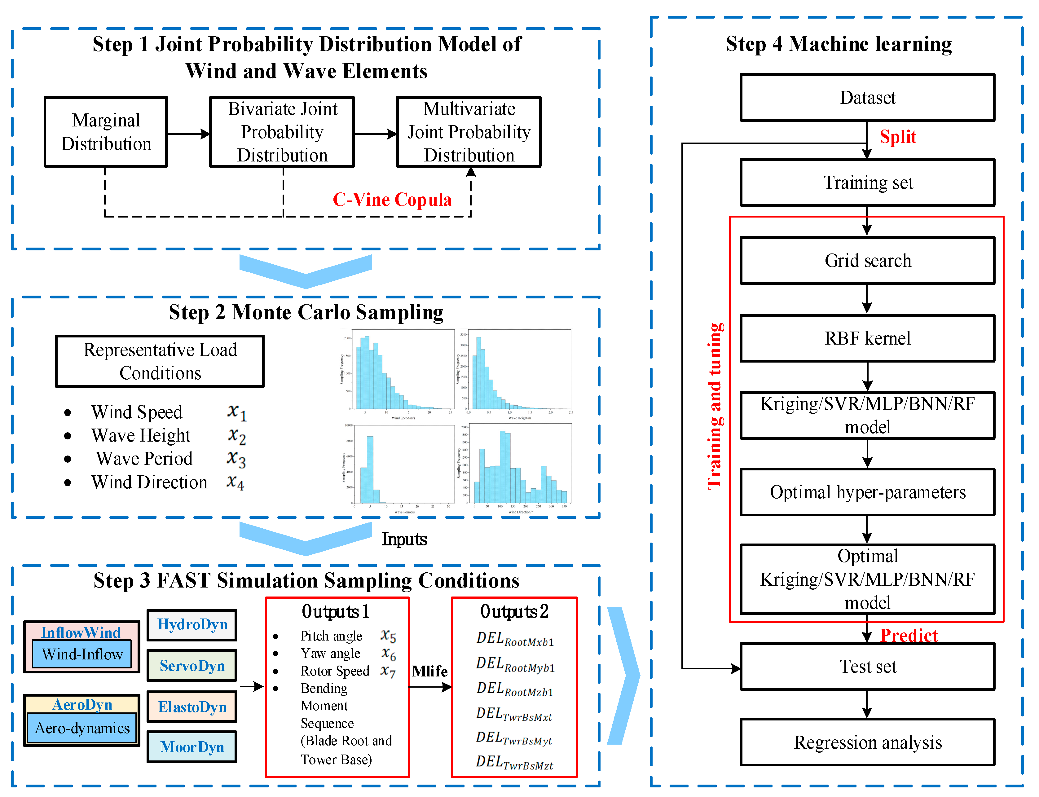
The fatigue load modeling method proposed in this study mainly includes three parts: (1) Establishing a four-dimensional joint probability distribution model of wind and wave variables based on Vine copula theory. (2) Determining representative wind and wave load conditions using the Monte Carlo sampling method. (3) Establishing a data-driven fatigue load model for floating wind turbines based on machine learning models. The schematic diagram of the methodology in this paper is shown in Figure 1. The abbreviated terms involved in the principle of the method proposed in this paper are listed in the Abbreviations section in the back matter.

2.1. Joint Probability Distribution Model of Wind and Wave Elements

To consider the long-term combined effects of wind and waves on FOWTs, this paper uses the C-Vine copula to construct the joint probability density function (PDF) of wind and wave variables. For clarity, a four-dimensional random variable is considered, and its probability density function can be expressed using the C-Vine copula structure as follows [28]:
f ( x 1 , x 2 , x 3 , x 4 ) = c 12 ( F 1 , F 2 ) c 13 ( F 1 , F 3 ) c 14 ( F 1 , F 4 ) c 23 | 1 ( F 2 | 1 , F 3 | 1 ) c 24 | 1 ( F 2 | 1 , F 4 | 1 ) × c 34 | 12 ( F 3 | 12 , F 4 | 12 ) f 1 f 2 f 3 f 4
Parameters involved in the calculation of C-Vine copula are shown in Table 1.
According to Equation (1), the joint probability density function is expressed as the product of the marginal probability density functions, marginal cumulative distribution functions, conditional marginal distributions, and a series of bivariate copula density functions. By establishing the marginal distribution models of the wind and wave variables, the marginal probability density functions, marginal cumulative distribution functions, and conditional marginal distributions can be obtained. Then, the optimal bivariate copula models are selected from the candidates to obtain their corresponding density functions, and the joint distribution of the wind and wave variables is established using the C-Vine structure. This paper models the marginal distribution and joint distribution separately.

2.1.1. Marginal Distribution Modeling

In marginal distribution modeling, common unimodal distribution models include the Weibull [29], Generalized Extreme Value (GEV) [30], and t-distribution with scale and location parameters [31]. Common multimodal distributions are often fitted using mixture models, such as the mixture Gamma distribution [32] and mixture Gaussian distribution [33].
When fitting these probability distribution models to the wind and wave variables, this paper employs maximum likelihood estimation for parameter estimation. To evaluate the goodness of fit of different probability distribution models, criteria such as AIC, BIC, and RMSE are used:
A I C = 2 i = 1 n l n f ( x i ) + 2 k
B I C = 2 i = 1 n l n f x i + k l n n
Parameters involved in the calculation of AIC and BIC are shown in Table 2.
R M S E = 1 n i = 1 n P c ( i ) P 0 ( i ) 2
Parameters involved in the calculation of RMSE are shown in Table 3. A smaller RMSE value indicates a better fit.

2.1.2. Joint Distribution Modeling

In the C-Vine copula method, establishing the joint distribution of multivariate variables involves three key steps: (1) determining the C-Vine copula structure configuration; (2) estimating parameters of the copula candidates; (3) conducting goodness-of-fit tests and selecting the optimal copula.
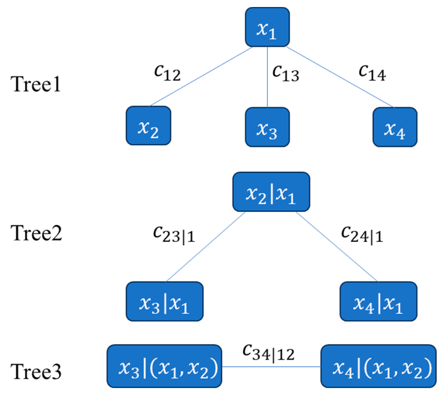
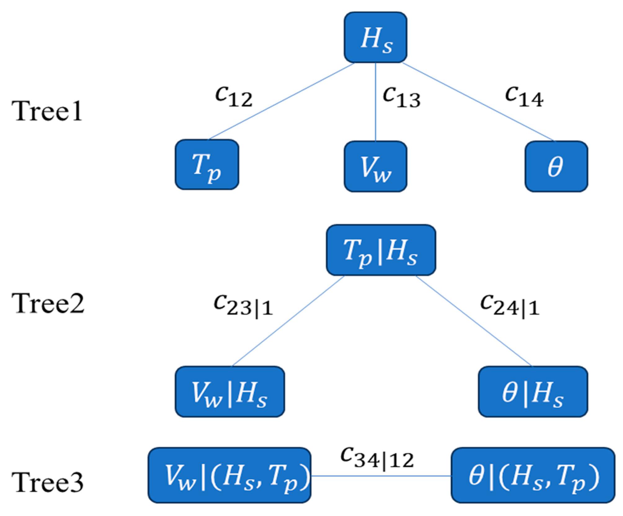
The structure configuration of the C-Vine copula adopts a tree-like structure, focusing on determining the order of root nodes and other nodes. The root node of the C-Vine copula is typically chosen based on its strongest correlation with other variables. This paper uses the sequential estimation method proposed by Aas et al. [28] to determine this. An example of the C-Vine copula tree structure for a four-dimensional random vector is shown in Figure 2. This configuration consists of three levels of trees, each with a main node. The main nodes are connected to other nodes through bivariate copulas, forming edges. These edges then serve as main nodes in the subsequent trees, continuing until all nodes connecting the trees are connected.
From Figure 2, after establishing the structure configuration of the C-Vine copula, it is necessary to determine the optimal bivariate copula corresponding to each edge in the structure. Various types of bivariate copulas are proposed in the literature [34], including Clayton copula, Frank copula, Gumbel copula, Gaussian copula, and Student’s t copula. Additionally, the BB8 copula [35], as a mixture copula combining characteristics of Clayton and Gumbel copulas, is designed to capture more complex dependency structures. The expression for the BB8 copula is as follows:
C ( u , υ ; θ , δ ) = e x p ( log u ) δ + ( log ν ) δ θ / δ
Parameters involved in the calculation of BB8 copula are shown in Table 4.
This paper considers Clayton copula, Frank copula, Gumbel copula, Gaussian copula, Student’s t copula, and BB8 copula functions as candidates for modeling the copula between pairwise variables in the C-Vine copula structure. Additionally, the Bayesian framework [36] and Gaussian likelihood based on residuals [37] are employed for parameter estimation.
To evaluate the goodness of fit of the selected copula functions, the root mean square error (e) is used as the criterion to assess the model’s performance, calculated by the formula below:
e = 1 n i = 1 n T ^ E u 1 i , u 2 i T u 1 i , u 2 i 2
T ^ E ( u 1 , u 2 ) = 1 n i = 1 n I ( u 1 i u 1 , u 2 i u 2 )
Parameters involved in the calculation of e are shown in Table 5. A smaller e indicates a better fit of the copula model to the empirical copula, reflecting closer agreement between them.

2.2. Monte Carlo Sampling Method

Previous studies often used grid-based methods to determine representative wind and wave conditions for fatigue load modeling [38]. The number of representative load conditions obtained by this method exponentially increases with the dimensionality of environmental variables, significantly increasing the computational burden. Therefore, this study employs a probability-based Monte Carlo sampling method to efficiently obtain representative wind and wave conditions in specific marine areas, which demonstrates significant advantages in terms of efficiency and convergence compared to grid-based methods [39].
Monte Carlo sampling is a numerical method that approximates complex probability distributions through extensive random sampling. In this study, Monte Carlo sampling is used to generate wind and wave condition samples that conform to the joint probability distribution model. In this process, all conditional samples have equal occurrence probabilities, i.e., p ( q i ) = 1 / N q ( i = 1 , . . . , N q ) . The specific sampling process is as follows:
Step 1: Input the joint probability distribution model. Assume the joint probability density function is f U V ( u , ν ) , where U , V are standardized marginal distribution variables of environmental factors such as wind speed, wave height, wave period, and wind direction;
Step 2: Random number generation. Generate two independent and uniformly distributed random numbers u i and ν i , where i = 1,2 , , N , and N is the number of samples;
Step 3: Use the inverse transform method to convert uniform random numbers into samples with specified marginal distributions. First, compute the cumulative distribution functions F U ( u ) and F V ( ν ) of the marginal distributions. Then, use the inverse functions F U 1 and F V 1 to transform the uniform random numbers u i and ν i into marginal distribution variables U i and V i :
U i = F U 1 ( u i ) ; V i = F V 1 ( υ i )
Step 4: Generate samples from the joint distribution. Use the copula function C ( u , υ ) from the Vine copula model to transform the marginal distribution samples U i and V i into samples from the joint distribution:
C ( u , υ ) = C ( F U ( u ) , F V ( ν ) )
Convert the generated samples ( U i , V i ) into physical quantities (such as wind speed, wave height, etc.).
After generating a large number of samples using Monte Carlo sampling, statistical analysis is applied to ensure the representativeness of these samples, covering all possible wind and wave conditions.

2.3. FAST Simulation and Fatigue Load Estimation Method

Given the complex fluid-structure-soil coupling system of floating offshore wind turbines, OpenFAST provides a high-fidelity offshore wind turbine model. Therefore, this paper uses OpenFAST to model a semi-submersible offshore wind turbine and conducts a high-fidelity analysis of its fatigue loads. Section 2.3.1 introduces the methods for performing aeroelastic simulations using the OpenFAST simulation environment, and Section 2.3.2 introduces the fatigue load assessment methods.

2.3.1. OpenFAST Simulation Method

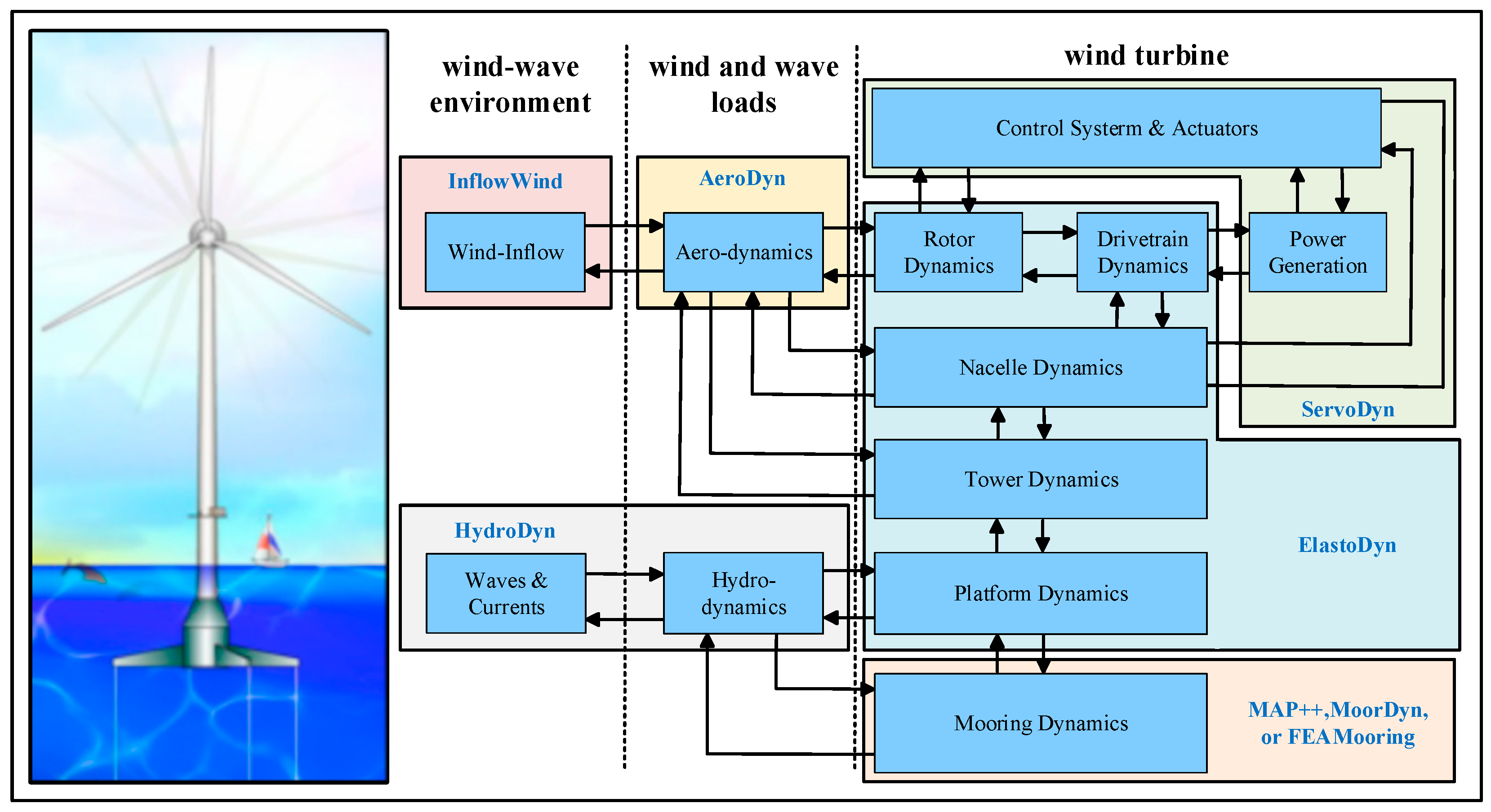
OpenFAST [40] is an open-source, high-fidelity, multiphysics (including aerodynamics, offshore hydrodynamics, control, and structural dynamics) aeroelastic simulation environment used to assess the coupled dynamic response of various wind turbine configurations, including onshore, bottom-fixed, or floating offshore topologies. Figure 3 provides an overview of the various components considered in the OpenFAST simulation. OpenFAST v3.1.0 and its earlier versions have been widely used in the literature for the simulation and analysis of onshore and offshore horizontal-axis wind turbines, offering high levels of detail and acceptability [41].
In this study, external environmental conditions are set using the InflowWind and HydroDyn modules. The generated wind and wave loads are coupled with the selected wind turbine using the ServoDyn, ElastoDyn, and MoorDyn modules for aeroelastic simulation, resulting in time series data of the bending moments of key components.

2.3.2. Fatigue Load Assessment Method

By post-processing the OpenFAST simulation results using the software tool MLife_v1.01 [42], the fatigue mechanical damage of key wind turbine components can be estimated. This tool has been applied in the literature to calculate fatigue mechanical loads related to active control strategies in HAWTs [43] or to determine the short-term mechanical impacts of sea waves on FOWT towers [44].
MLife weights the fatigue damage equivalent loads (DEL) for each moment unit based on statistical terms given by the Weibull distribution and its characteristic parameters, scale, and shape, which determine the occurrence frequency of each wind speed interval [45]. For onshore wind turbines, the probability of wind occurrence might be sufficient to calculate long-term fatigue damage. However, for offshore wind turbines, the statistical distribution of sea states must also be considered to obtain reliable results.
The steps to calculate damage equivalent loads are as follows: First, the rainflow counting method is used to decompose fluctuating loads into individual hysteresis cycles by matching local peaks and valleys. Then, based on the number of fatigue cycles and the Palmgren-Miner rule, the damage equivalent loads are calculated, representing constant amplitude fatigue loads generated at fixed load means and frequencies. The calculation formula is as follows:
D E L j S T = i ( n j i ( L j i R ) m ) n j S T e q 1 m
n j S T e q = f e q T j
Parameters involved in the calculation of DEL are shown in Table 6. Specifically, for the tower, LSS, and mooring cables, m takes values of 3, 4, and 5, respectively, while for the blades, m assumes values of 8, 10, and 12 [19]. Additionally, D E L j S T stands for the short-term DEL for time series j with a fixed mean.

2.4. Machine Learning-Based Fatigue Load Modeling Method

This study selects five machine learning models—Kriging, MLP, SVR, BNN, and RF—to establish a fatigue load model for FOWTs. The choice of these models is based on their successful applications in similar tasks and their respective theoretical advantages.
Kriging is a non-parametric model suitable for handling spatial correlations in small-sample data, capable of providing predictions and estimating prediction uncertainties [46]. MLP utilizes nonlinear activation functions in its hidden layers to capture nonlinear relationships in data, offering strong approximation capabilities and flexibility [47]. SVR minimizes generalization error by maximizing the margin and uses kernel techniques to handle complex nonlinear relationships, demonstrating robustness against outliers and noise [48]. BNN combines Bayesian inference with neural networks, applying Bayesian methods for regularization to prevent overfitting [49]. RF, through ensemble learning of multiple decision trees, effectively reduces overfitting risks and generally provides excellent prediction accuracy across various tasks, with a high tolerance for data noise and missing values [50].
Through comprehensive evaluation of these models, the optimal model for the current task of fatigue load modeling for floating wind turbines can be selected. The algorithm pseudocode for evaluating and selecting the best model among the five is provided in Algorithm 1, outlining a complete framework from data preprocessing and correlation analysis to training and evaluation of machine learning models. Initially, compute correlations between wind and wave environmental variables, turbine operational states, and equivalent damage loads. Next, select the four variables most correlated with equivalent damage loads as inputs for machine learning models. Then, initialize and train the five different machine learning models (Kriging, MLP, SVR, BNN, and RF) using the selected input variables to predict equivalent damage loads. Finally, assess each model’s performance using appropriate metrics such as Mean Squared Error (MSE), outputting predicted equivalent damage loads and evaluation metrics for comparison and analysis.
Algorithm 1 Damage Equivalent Load (DEL) Prediction and Model Selection
Input:
  Environment variables: wind_speed, wave_height, wave_period, wind_direction
  Turbine state variables: yaw_angle, rotor_speed, blade_pitch
  DEL: RootMxb1, RootMyb1, RootMzb1, TwrBsMxt, TwrBsMyt, TwrBsMzt
Output:
  Best model among Kriging, MLP, SVR, BNN, RF based on overall error
1. Correlation Analysis:
 Compute correlation coefficients between:
   - wind_speed, wave_height, wave_period, wind_direction
   - yaw_angle, rotor_speed, blade_pitch
  and
   - RootMxb1, RootMyb1, RootMzb1, TwrBsMxt, TwrBsMyt, TwrBsMzt
2. Select Input Variables:
 Select top four variables with highest absolute correlation coefficients with DEL:
   - selected_input_variables = [var1, var2, var3, var4]
3. Machine Learning Models Training and Prediction:
 Initialize models: Kriging, MLP, SVR, BNN, RF
for each model in [Kriging, MLP, SVR, BNN, RF]:
   Train model using selected_input_variables to predict DEL values:
    - model.train(X_train[selected_input_variables], y_train[DEL])
   Predict DEL values for test dataset:
    - predicted_DEL = model.predict(X_test[selected_input_variables])
   Calculate overall error (e.g., MSE) for the model:
    - overall_error = calculate_error(predicted_DEL, y_test[DEL])
   Store model and its overall error
4. Select Best Model:
 Identify model with minimum overall error:
   - best_model = model with minimum overall_error
5. Output Results:
 Print or store predicted DEL values and evaluation metrics for best_model.
End Algorithm

2.5. Framework for Fatigue Load Modeling of Floating Wind Turbines

Figure 4 illustrates the framework proposed for fatigue load modeling of floating wind turbines, comprising four main stages:
(1)
Establishment of joint probability distribution models for wind and wave factors: Marginal distribution model parameters for each wind and wave factor are determined using maximum likelihood estimation. The goodness of fit is evaluated using AIC, BIC, and RMSE criteria to establish marginal distributions of wind and wave factors. Subsequently, parameters of the two-dimensional copula function are estimated within a Bayesian framework using a Gaussian likelihood function based on residuals, with model selection based on AIC for optimal copula function determination. Finally, the C-Vine copula theory is employed to establish a joint probability distribution model for the four-dimensional random variables: wind speed, wave height, wave period, and wind direction;
(2)
Monte Carlo sampling for representative sample conditions: Following construction of the joint PDF of ocean environmental variables, Monte Carlo sampling is employed to obtain representative sample conditions of wind speed ( x 1 ), wave height ( x 2 ), wave period ( x 3 ), and wind direction ( x 4 ) as input conditions for subsequent simulation modeling;
(3)
FAST simulation under-sampled conditions: To establish a data-driven model for fatigue load data at critical components such as blade roots and tower bases of floating wind turbines, a substantial volume of effective data is required to build the database. Post identification of representative load conditions, OpenFAST is utilized to model fatigue loads for all sampled conditions;
(4)
Machine learning-based damage equivalent load modeling: Machine learning techniques are employed to construct fatigue load models. Model inputs include environmental variables (wind speed, wave height, wave period, wind direction) and operational state variables (rotor speed, yaw angle, blade pitch angle). Outputs consist of damage equivalent loads for six key moments at blade roots (RootMxb1, RootMyb1, and RootMzb1) and tower bases (TwrBsMxt, TwrBsMyt, and TwrBsMzt).

3. Case Study

3.1. Study Object

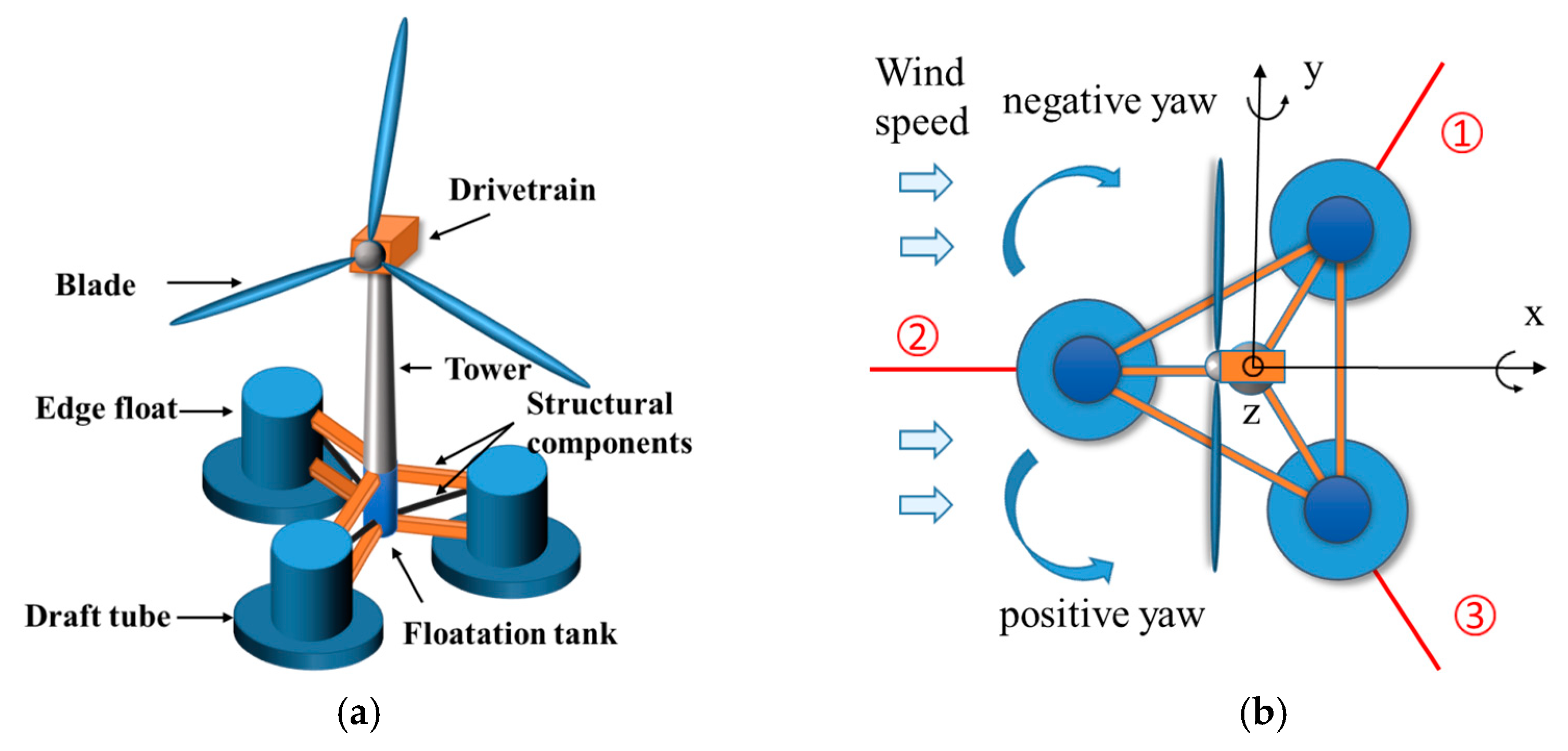
Different marine environments lead to varying stress deformation and fatigue damage in wind turbines. Investigating the performance of FOWT in different marine environments requires numerical simulation methods or experimental approaches. This paper employs the OpenFAST numerical simulation software developed by the U.S. National Renewable Energy Laboratory (NREL) for simulation, focusing on their 5 MW semi-submersible offshore wind turbine. The turbine structure is depicted in Figure 5, and key parameters can be found in reference [51].

3.2. Analysis of Joint Probability Distribution Modeling Results of Wind and Wave Factors

3.2.1. Data Description

The study utilizes oceanographic and meteorological observation data from the Lianyungang Marine Observation Station in the East China Sea for the years 2018–2022. The data are provided by the National Marine Data and Information Service Center of China (http://mds.nmdis.org.cn/). Selected wind and wave elements include average wind speed at 10 m height, wave height, wave period, and wind direction. These parameters are measured hourly, and the station’s coordinates are 34°47′0″ N 119°26′0″ E. It should be noted that during data processing, a small portion of the observational data from the marine station was found to be missing, meaning some elements were occasionally not observed. To address this, missing sample data was excluded to retain as many remaining data samples as possible, resulting in a total of 37,892 datasets.
Wind speed at 10 m height ( U 10 ), wind direction ( U d i r ), wave period ( T p ), and wave height ( H s ) are the focus of this study. The reference NREL 5 MW wind turbine hub height is 90 m. Therefore, an exponential profile method [45] is used to convert the wind speed at 10 m height to 90 m height, with the calculation formula as follows:
U 90 = U 10 × ( H 90 m H 90 m ) α
where α is the wind profile exponent coefficient, set to 0.12.
Additionally, only marine meteorological data with wind speeds within the operational range (3–25 m/s) are considered conducive to fatigue damage. Consequently, the final dataset comprises 29,777 samples.

3.2.2. Results of Marginal Distribution Modeling

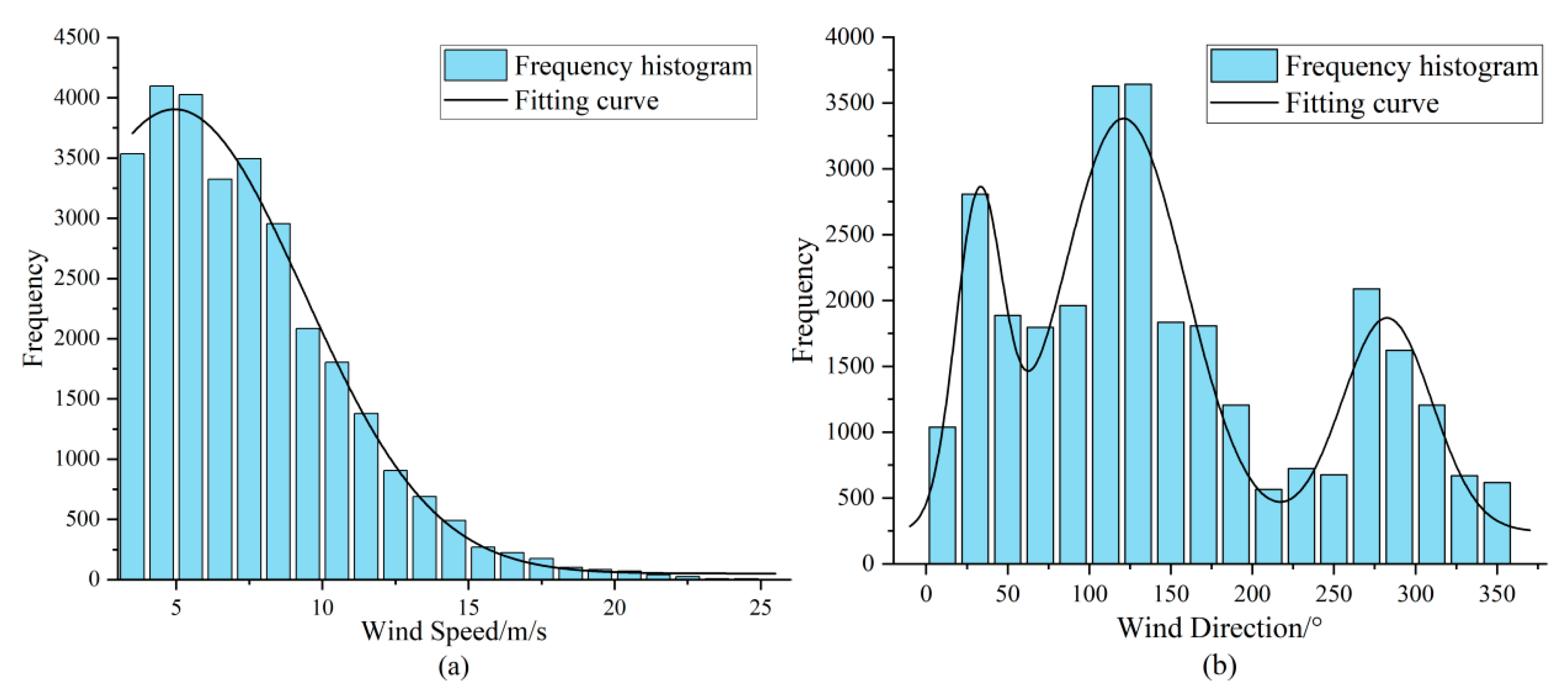
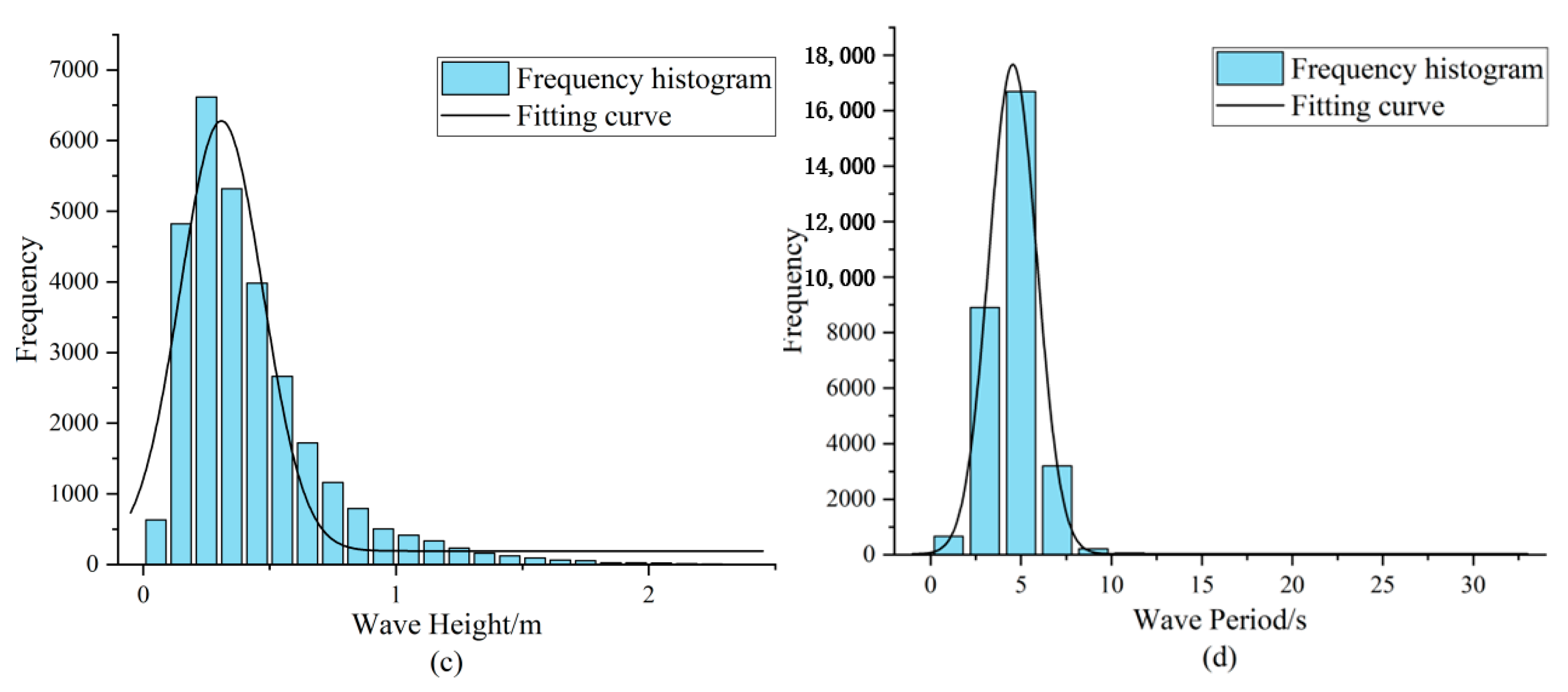
Figure 6a–d depicts frequency histograms and fitted curves of measured wind and wave data from Lianyungang. It is observed that wind speed, wave height, and wave period samples exhibit characteristics of unimodal distributions (Figure 6a–c), fitted using common unimodal distribution models. Wind direction shows a multimodal distribution (Figure 6d) fitted using a mixture model. Additionally, the probability histogram of wind direction reveals three distinct peaks in its distribution. Therefore, a mixture model with three unimodal distribution functions is employed to fit the data, resulting in a mixture model with three dimensions.
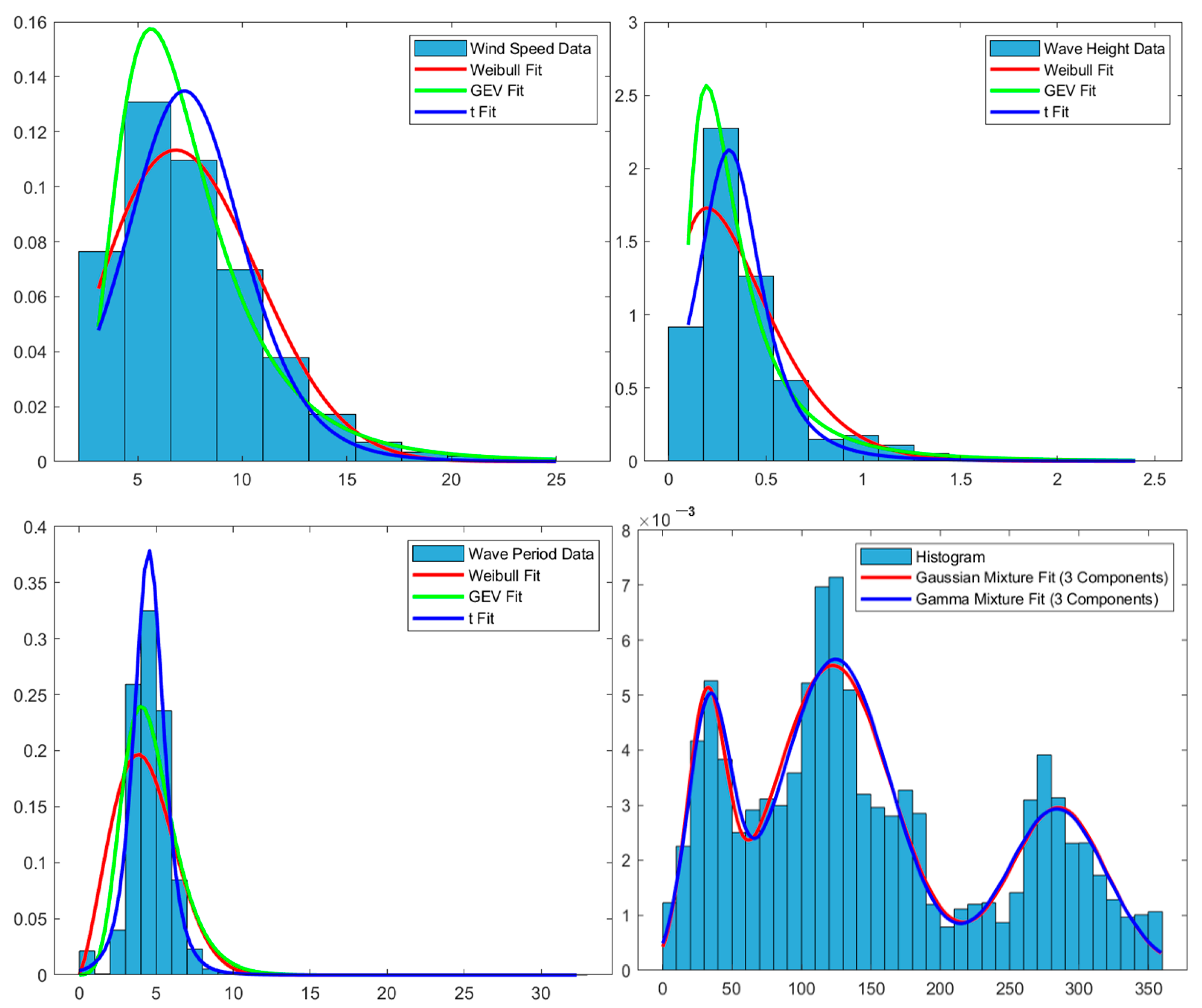
Table 7 and Table 8 present the different marginal probability distribution types and corresponding parameters for the four wind and wave factors: wind speed, wave height, wave period, and wind direction. According to the goodness-of-fit evaluation results in Table 8 and Table 9, the optimal fitting distributions for wind speed, wave height, and wave period are the Weibull distribution, the Generalized Extreme Value (GEV) distribution, and the t-distribution with location and scale parameters, respectively. The optimal fitting distribution for wind direction is the mixed Gaussian distribution. Figure 7 shows the histograms of the samples for these four wind and wave factors and the fitting curves of three marginal probability distributions. It can be seen that the selected optimal marginal probability distribution curves fit the samples of the four wind and wave factors well.

3.2.3. Joint Distribution Modeling Results

The C-Vine copula, outlined in Section 2.1.2, is used to simulate the joint distribution of wind and wave variables. Table 9 displays the empirical Kendall correlation coefficients for all pairwise combinations of random variables. These coefficients guide the selection of root nodes and the order of other nodes within each layer of the C-Vine structure. Figure 8 illustrates the optimal C-Vine copula structure for the wind and wave variables. Here, H s represents significant wave height, T p represents wave period, V w represents wind speed, and θ represents wind direction.
Then, Gaussian, Frank, Gumbel, Student’s t, Clayton, and BB8 copula functions were considered as candidate models for modeling the dependence structure of paired variables. In this case, the identified optimal bivariate copula is shown in Table 10.
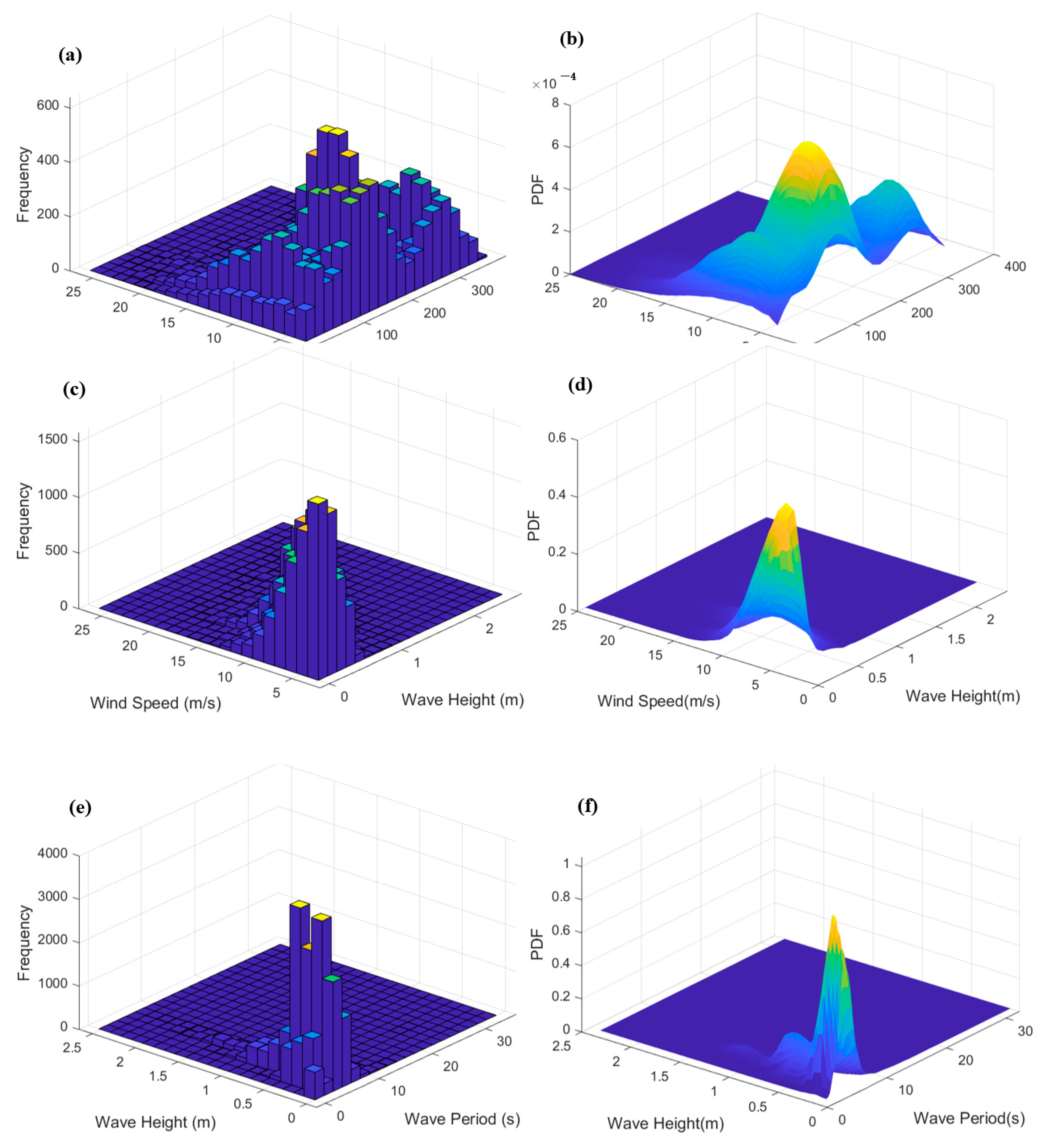
The two-dimensional frequency histograms and joint distribution probability density plots in Figure 9 visually demonstrate the fitting effectiveness of the optimal bivariate copula models selected in this study. For wind speed—wave height, wind speed—wind direction, and wave height—wave period, the peaks and shapes of the two-dimensional joint probability density plots closely match those of the two-dimensional frequency histograms. This indicates a reasonable simulation of correlations, effectively considering the dependencies among wind and wave variables.
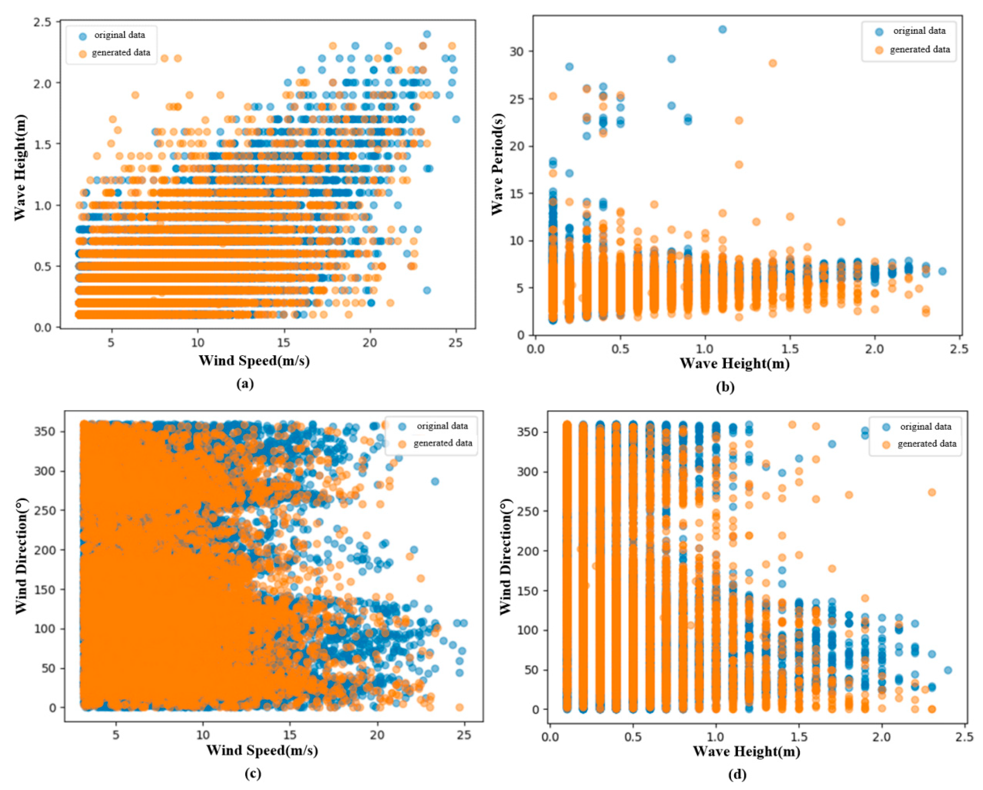
Using the established C-Vine model, cumulative probability densities of the four-dimensional random variables—wind speed, wave height, wave period, and wind direction—were simulated. The comparison between generated samples and original data is shown in Figure 10. From the figure, it can be observed that the probabilistic dependency characteristics of the generated samples closely match those of the original data. Furthermore, performing a K-S test between the generated samples and original data yielded a K-S test statistic of 0.0025 and a K-S test p-value of 0.9917. This indicates that not only are the distributions of the generated samples and original data very similar (low K-S test statistic) but also the p-value exceeds 0.05, failing to reject the null hypothesis, demonstrating no significant difference between the two distributions. Therefore, the C-Vine copula model developed in this section effectively represents the joint distribution of environmental variables in the studied marine region.

3.3. Analysis of Fatigue Load Modeling Based on Machine Learning

Based on the joint probability distribution model constructed in Section 3.2, representative wind and wave conditions were determined using the Monte Carlo method. TurbSim [52] and the HydroDyn module in FAST were used to generate representative wind and wave conditions as inputs for OpenFAST simulation. After determining simulation parameters and conducting correlation analysis, input and output variables for the machine learning model were identified. Five commonly used machine learning algorithms were employed to construct the data-driven model.

3.3.1. Simulation Parameter Settings and Correlation Analysis

This study primarily considers the fatigue loads on the blade root and tower base of a Floating Wind Turbine. Representative load conditions were determined using the Monte Carlo sampling method, with results shown in Figure 11. Wind turbine design standards recommend at least six 10-min simulations per random seed [53], whereas, for beam-type FOWTs, simulations typically extend to 60 min in total length [54]. Therefore, this research adopted a simulation length of 1200 s and used three random seeds. To eliminate transient responses, an additional 300 s of simulation time was considered at the start of each simulation, with fatigue analysis based solely on the subsequent 1200 s of simulation results. Thus, OpenFAST conducted sub-simulations with a total simulation time of 1500 s while recording yaw angle, pitch angle, generator speed, tower base bending moments in three directions, and blade root bending moments in three directions.
To establish a data-driven model for the DEL of floating wind turbines, suitable and easily measurable variables need to be selected as inputs. In this study, Mlife [45] was used to compute the DEL values for moments. Considering the studied object, a total of seven variables were selected, including wind and wave environmental variables (wind speed, wave height, wave period, wind direction) and wind turbine operational states (yaw angle, rotor speed, blade pitch angle). To analyze the correlation between the selected inputs and DEL, Pearson correlation coefficients (PCC) between wind and wave environmental variables and DEL were calculated, as shown in Figure 12. It is evident that among the environmental variables, wind speed and wave height exhibit higher correlations with DEL at the root and tower base compared to wave period and wind direction. Pearson correlation coefficients (PCC) between wind turbine operational state variables and DEL are shown in Figure 13. It is observed that among the operational state variables, generator speed variance and nacelle yaw angle variance show high correlations with DEL of the root and tower base moments, with a Pearson correlation coefficient as high as 0.9227. In contrast, the correlation with blade pitch angle is minimal, with a Pearson correlation coefficient below 0.1. In summary, combining wind and wave variables with operational state variables, this study selects wind speed, wave height, generator speed variance, and nacelle yaw angle variance as the four variables for the data model inputs, and DEL of RootMxb1, RootMyb1, RootMzb1, TwrBsMxt, TwrBsMyt, and TwrBsMzt as the outputs of the data model.

3.3.2. Modeling Results of Data-Driven Models

This study randomly selected 10,000 data points as the training set and the remaining 5000 data points as the test set. Mean squared error (MSE) was used to evaluate the model accuracy. The configurations and optimization methods of five machine-learning models are shown in Table 11.
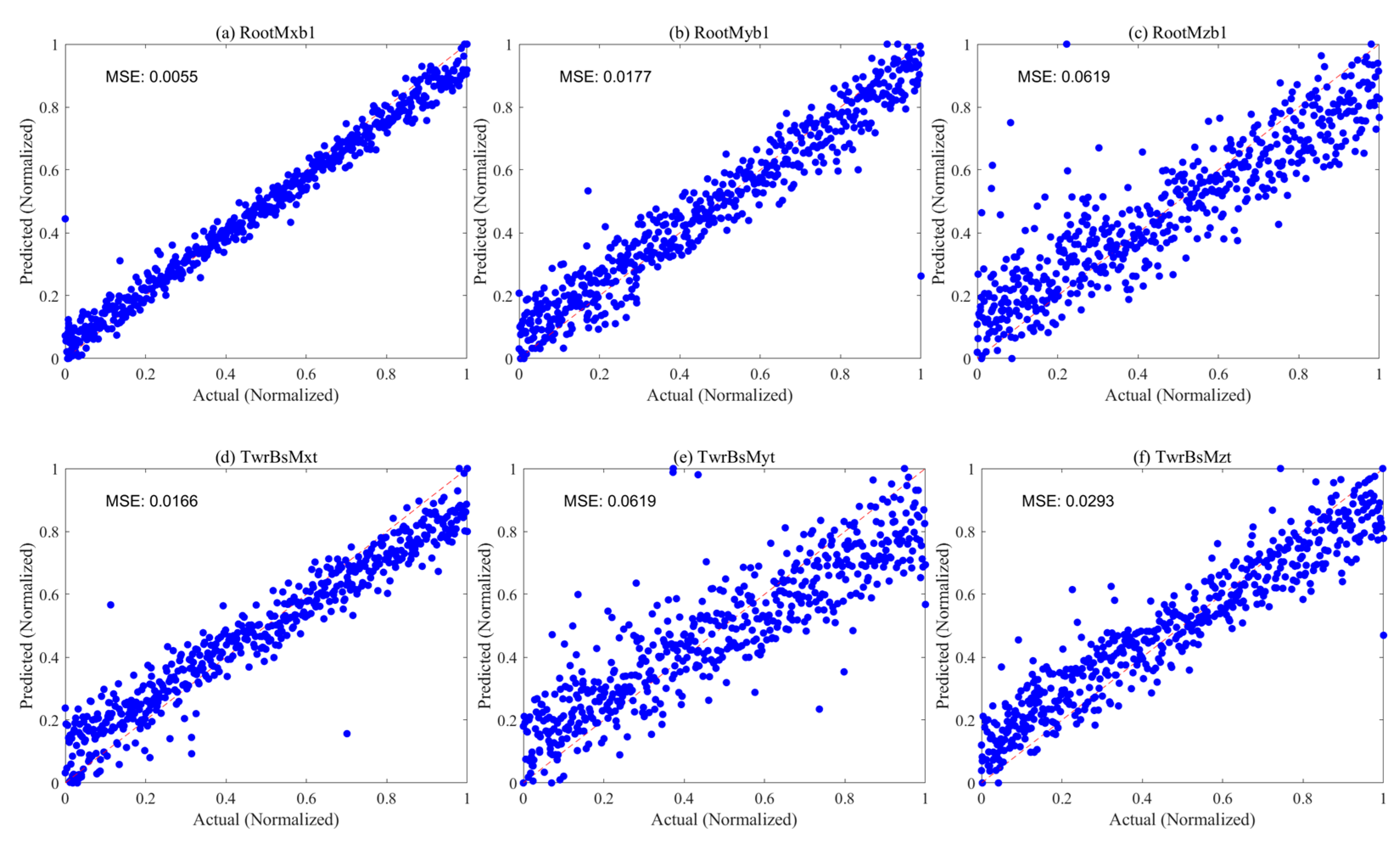
Figure 14 illustrates the regression capability of the Kriging model for six outputs. In Figure 14a, the Kriging model demonstrates excellent predictive performance for RootMxb1 DEL, achieving a high accuracy of 99.45%. In Figure 14b,d,f, the model achieves DEL prediction accuracies greater than 97% for RootMyb1, TwrBsMxt, and TwrBsMzt, respectively, which are slightly lower compared to RootMxb1. However, for RootMzb1 and TwrBsMyt, the Kriging model shows slightly lower prediction accuracy at 93.81%, possibly due to its performance degradation in high-dimensional spaces.
Figure 15 illustrates the regression capabilities of the MLP model for the six outputs. For the DEL prediction of RootMxb1, the MSE value is 0.2593, indicating a significant prediction bias. Additionally, the prediction accuracy for the DEL values of the other five moments did not reach an optimal level, with prediction accuracies falling below 90%. This suggests that although the MLP model has certain advantages in capturing the nonlinear characteristics of the data, its performance is still constrained by the complexity of the fatigue load prediction task and the inherent noise within the data.
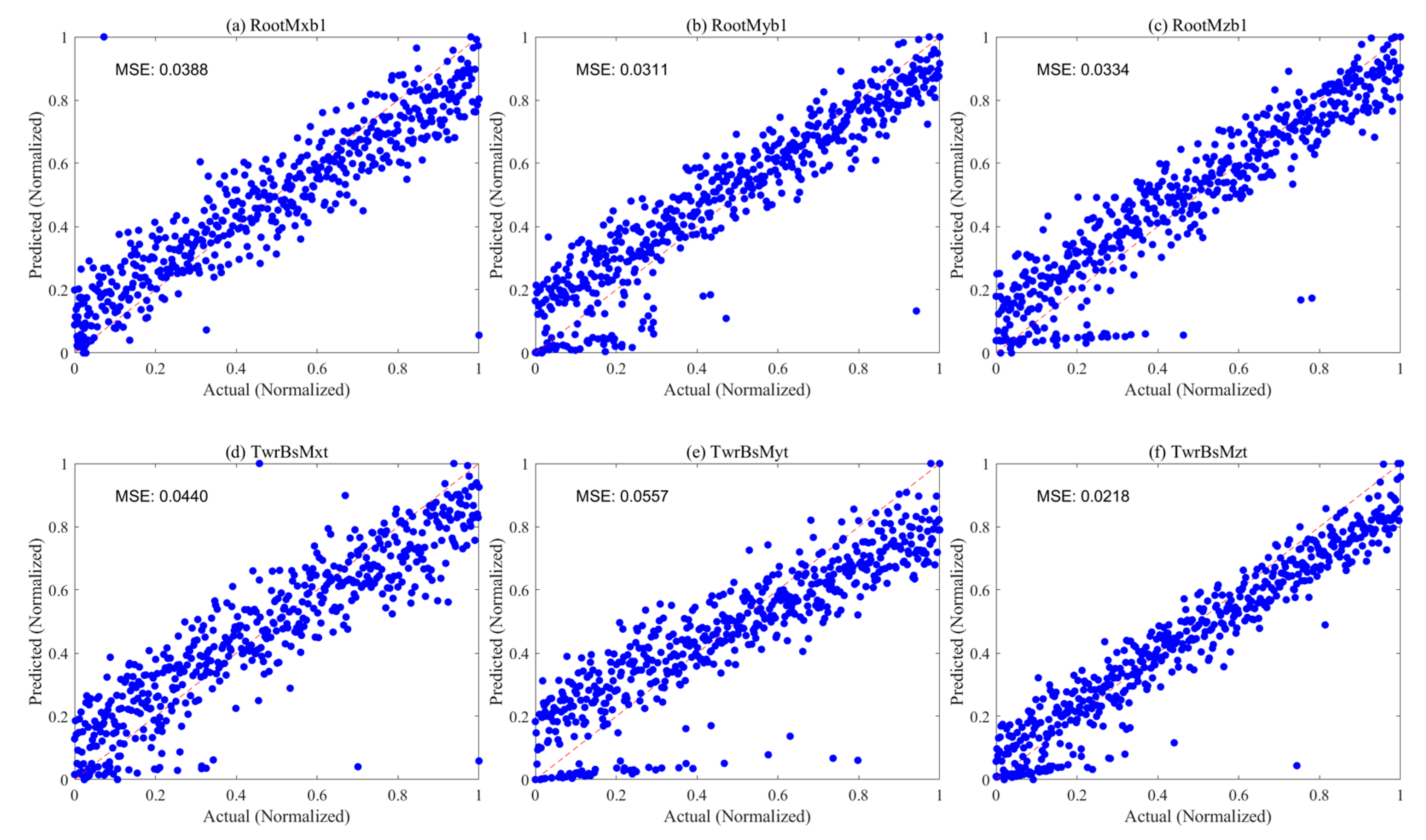
Figure 16 demonstrates the regression capabilities of the SVR model for the six outputs. It is evident that the prediction accuracy for all six outputs exceeds 94.43%, reaching up to 97.82%. This indicates that the SVR model exhibits strong generalization ability in handling high-dimensional data and regression tasks. However, compared to the Kriging model and the subsequent RF model, the SVR model still shows some gaps in performance, revealing its limitations in capturing extreme data features.
Figure 17 illustrates the regression capabilities of the BNN model for the six outputs. It is evident that, compared to the Kriging, MLP, SVR, and subsequent RF models, the BNN model has prediction accuracies for all six outputs below 89.86%. Particularly in predicting the damage equivalent load values in the lateral directions of the tower base, the BNN model shows substantial errors, with a mean squared error value of 0.3939. This indicates that while the BNN may have some advantages in capturing simple linear relationships, its performance in handling complex nonlinear regression tasks is constrained by the simplicity of its structure and the number of neurons.
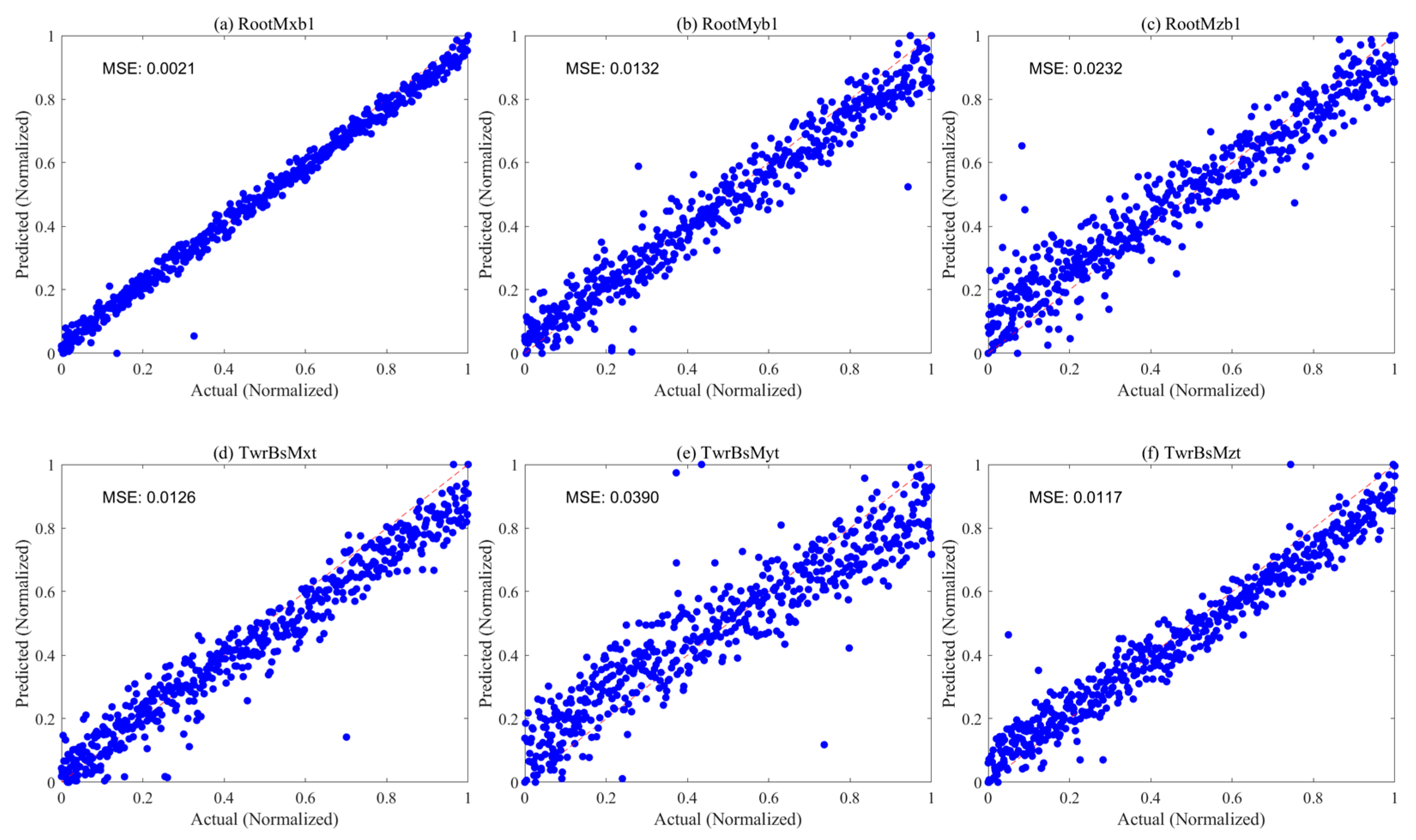
Figure 18 illustrates the regression capabilities of the RF model for the six outputs. It can be concluded that the overall regression performance is quite satisfactory, with very low MSE values for fatigue load predictions from the blade to the tower base and the maximum prediction error being just 3.9%. Notably, for the fatigue load at the blade root, the DEL prediction for RootMxb1 is nearly accurate, with a prediction accuracy of 99.97%. Compared to the previous four models, the RF model demonstrates the best performance in predicting the DEL values for these six moments, showcasing its strong capability in handling complex data and capturing nonlinear features.
Table 12 presents the MSE, RMSE, and R 2 values for the six output moment DEL values from the five machine learning models and the traditional polynomial regression model. It is evident that, overall, the RF, Kriging, and SVR models exhibit better predictive performance, whereas the MLP and BNN models have relatively higher prediction errors, with the polynomial regression model exhibiting the highest errors. Specifically, the traditional polynomial regression model consistently shows MSE and RMSE values greater than 1 and R 2 values less than 0.2, compared to the five machine learning models, indicating larger prediction errors. Among the five machine learning models, the RF model achieves MSE values less than 0.05 and RMSE values less than 0.2 for all six-moment DELs, with R 2 values greater than 0.95. This demonstrates that the RF model performs best in predicting fatigue loads for the blade root and tower base of floating wind turbines, making it the optimal choice for developing prediction models for blade root and tower base moment DELs.
Overall, using machine learning methods for modeling fatigue loads in floating wind turbines is significantly advantageous. Machine learning can efficiently handle complex multivariate data, thereby enhancing modeling accuracy and predictive performance. This provides new solutions for wind energy engineering, demonstrating broad application prospects in predicting fatigue loads of floating wind turbines and optimizing offshore wind farm operations.

4. Conclusions

This paper proposes a method for modeling fatigue loads of floating wind turbines based on Vine copula theory and machine learning. The aim is to establish a fatigue load model for floating wind turbines using marine meteorological data as a basis for optimizing their operation. Against the backdrop of real wind and wave data from marine sites, a C-Vine copula structure is utilized to establish joint probability density functions between wind and wave elements at these sites. Subsequently, representative load conditions are obtained through Monte Carlo sampling. Five machine learning models—Kriging, MLP, BNN, SVR, and RF—are trained, and their performance is compared and analyzed, leading to the following conclusions:
(1)
Detailed analysis of measured data from the Lianyungang marine site in the East China Sea reveals that wind speed, wave height, and wave period exhibit unimodal distribution characteristics suitable for fitting with common unimodal distribution models, whereas wind direction shows multimodal distribution characteristics requiring a mixture model for fitting. Specifically, the optimal fitting distributions are the Weibull distribution for wind speed, Generalized Extreme Value (GEV) distribution for wave height, t-distribution with scale parameter for wave period, and mixed Gaussian distribution for wind direction. The Root Mean Square Error for fitting these four variables is all less than 0.01, indicating the good performance of the selected optimal marginal probability distribution models in fitting;
(2)
The established C-Vine copula model effectively characterizes the joint probability distribution between the four-dimensional random variables of wind speed, wave height, wave period, and wind direction. Specifically, comparing the probability dependency characteristics of model-generated samples with original data reveals a high degree of consistency between the two. Additionally, the Kolmogorov–Smirnov (K-S) test statistic of 0.0025 indicates that the distribution of generated samples is nearly identical to that of the original data. The K-S test p-value of 0.9917 further confirms that there is no significant difference between generated samples and original data. These results demonstrate the reliability and effectiveness of the model in simulating environmental variables;
(3)
For predicting fatigue loads of floating wind turbine root and tower base moments, the RF model demonstrates superior prediction performance and generalization ability, achieving outstanding results with a minimum MSE of only 0.0021 for predicting six DEL values. While the Kriging model approaches the accuracy of the RF model on some variables, it exhibits slight degradation in high-dimensional spaces. In contrast, MLP and BNN models show higher prediction errors, especially the BNN model with an MSE exceeding 0.3 in some predictions, indicating limited prediction accuracy. Therefore, it is recommended that the RF model be selected as the preferred method for establishing DEL prediction models for root and tower base moments in practical applications, ensuring the accuracy and reliability of prediction results.
Our research results provide practical guidance for enhancing the structural reliability and operational efficiency of floating wind turbines. By employing advanced statistical techniques and machine learning, our approach helps mitigate operational risks in offshore wind farms and optimizes energy production. Furthermore, our study not only advances the field of fatigue load modeling for floating wind turbines but also establishes a foundation for integrating complex environmental data with advanced modeling techniques. This comprehensive approach holds promise for driving innovation and resilience in offshore wind energy systems, contributing to the future of sustainable energy.
Although further research is needed for modeling fatigue loads of floating wind turbines at other marine observation sites, the proposed method and approach in this paper provide valuable insights for such research. Future studies can validate and refine this method in more diverse marine environments and conditions to further enhance the accuracy and applicability of the model.

Author Contributions

Methodology, X.Y. and E.X.; Software, X.Y.; Validation, Q.H.; Formal analysis, Q.H. and E.X.; Resources, D.S., Z.X., J.Y. and S.E.; Data curation, E.X.; Writing—original draft, X.Y.; Writing—review & editing, D.S., Z.X., J.Y., M.D., R.W., S.E. and Y.-H.J.; Supervision, D.S., J.Y., M.D. and R.W.; Project administration, D.S., S.E. and Y.-H.J.; Funding acquisition, D.S., Z.X., J.Y. and Y.-H.J. All authors have read and agreed to the published version of the manuscript.

Funding

This research is supported under the framework of international cooperation program managed by National Natural Science Foundation of China under Grant 62211540397 and the National Research Foundation of Korea (NRF-2022K2A9A2A06045121), the Natural Science Foundation of Hunan Province (Grant Nos. 2021JJ30875, 2022JJ90003 and 2022JJ90012), the Science and Technology Innovation Program of Hunan Province (2023RC3174), and the Natural Science Foundation of Changsha (kq2208288).

Institutional Review Board Statement

Not applicable.

Informed Consent Statement

Not applicable.

Data Availability Statement

Data are contained within the article.

Conflicts of Interest

The authors declare no conflicts of interest.

Abbreviations

FOWTFloating Offshore Wind Turbine
C-Vine copulaCanonical Vine copula
CDFCumulative Distribution Function
PDFProbability Density Function
GEVGeneralized Extreme Value distribution
AIC Akaike Information Criterion
BICBayesian Information Criterion
RMSEEvaluate the goodness of fit of different probability distribution models
C ( u , υ ; θ , δ ) The expression for the BB8 copula
e Evaluate the goodness of fit of the selected copula functions
KrigingGeostatistical Kriging
MLPMultilayer Perceptron
SVRSupport Vector Regression
BNNBayesian Neural Network
RFRandom Forest
DELDamage Equivalent Load
var1, var2, var3, var4Marine environmental variables 1, 2, 3, and 4, respectively
RootMxb1Edgewise bending moment at the blade root
RootMyb1Flapwise bending moment at the blade root
RootMzb1The z-directional bending moment at the blade root
TwrBsMxtSide-side (or roll) bending moment at the tower base
TwrBsMytFore-aft (or pitch) bending moment at the tower base
TwrBsMztThe z-directional bending moment at the tower base
MSE/RMSE/ R 2 Evaluate machine learning model errors

References

  1. Global Wind Energy Council. Global Wind Report 2023. Available online: https://gwec.net/globalwindreport2023/ (accessed on 1 November 2023).
  2. Global Wind Energy Council. Global Wind Report 2024. Available online: https://gwec.net/global-wind-report-2024/ (accessed on 20 June 2024).
  3. Robertson, B.; Dunkle, G.; Gadasi, J.; Garcia-Medina, G.; Yang, Z. Holistic marine energy resource assessments: A wave and offshore wind perspective of metocean conditions. Renew. Energy 2021, 170, 286–301. [Google Scholar] [CrossRef]
  4. Offshore Wind Energy (OWE). Technology of OWE. 2009. Available online: http://www.offshorewindenergy.org/ (accessed on 26 July 2024).
  5. Alkhabbaz, A.; Hamza, H.; Daabo, A.M.; Yang, H.S.; Yoon, M.; Koprulu, A.; Lee, Y.H. The aero-hydrodynamic interference impact on the NREL 5-MW floating wind turbine experiencing surge motion. Ocean Eng. 2024, 295, 116970. [Google Scholar] [CrossRef]
  6. Edirisinghe, D.S.; Yang, H.S.; Gunawardane, S.; Alkhabbaz, A.; Tongphong, W.; Yoon, M.; Lee, Y.H. Numerical and experimental investigation on water vortex power plant to recover the energy from industrial wastewater. Renew. Energy 2023, 204, 617–634. [Google Scholar] [CrossRef]
  7. Guo, Y.; Wang, H.; Lian, J. Review of integrated installation technologies for offshore wind turbines: Current progress and future development trends. Energy Convers. Manag. 2022, 255, 115319. [Google Scholar] [CrossRef]
  8. Bitner-Gregersen, E.M.; Dong, S.; Fu, T.; Ma, N.; Maisondieu, C.; Miyake, R.; Rychlik, I. Sea state conditions for marine structures’ analysis and model tests. Ocean Eng. 2016, 119, 309–322. [Google Scholar] [CrossRef]
  9. Czado, C.; Nagler, T. Vine copula based modeling. Annu. Rev. Stat. Its Appl. 2022, 9, 453–477. [Google Scholar] [CrossRef]
  10. Li, X.; Zhang, W. Long-term assessment of a floating offshore wind turbine under environmental conditions with multivariate dependence structures. Renew. Energy 2020, 147, 764–775. [Google Scholar] [CrossRef]
  11. Zhao, Y.; Dong, S. Multivariate probability analysis of wind-wave actions on offshore wind turbine via copula-based analysis. Ocean Eng. 2023, 288, 116071. [Google Scholar] [CrossRef]
  12. Det Norske Veritas. Environmental Conditions and Environmental Loads; Det Norske Veritas: Oslo, Norway, 2000. [Google Scholar]
  13. Sutherland, H.J. On the Fatigue Analysis of Wind Turbines. 1999. Available online: https://www.osti.gov/biblio/9460 (accessed on 30 November 2023).
  14. Offshore Standard DNV-OS-J101; Design of Offshore Wind Turbine Structure. Det Norske Veritas: Oslo, Norway, 2004.
  15. Yang, J.; Zheng, S.; Song, D.; Su, M.; Yang, X.; Joo, Y.H. Data-driven modeling for fatigue loads of large-scale wind turbines under active power regulation. Wind Energy 2021, 24, 558–572. [Google Scholar] [CrossRef]
  16. He, R.; Yang, H.; Lu, L. Optimal yaw strategy and fatigue analysis of wind turbines under the combined effects of wake and yaw control. Appl. Energy 2023, 337, 120878. [Google Scholar] [CrossRef]
  17. Woo, S.; Park, J.; Park, J. Predicting wind turbine power and load outputs by multi-task convolutional LSTM model. In Proceedings of the 2018 IEEE Power & Energy Society General Meeting (PESGM), Portland, OR, USA, 5–10 August 2018; pp. 1–5. [Google Scholar]
  18. Yao, Q.; Ma, B.; Zhao, T.; Hu, Y.; Fang, F. Optimized active power dispatching of wind farms considering data-driven fatigue load suppression. IEEE Trans. Sustain. Energy 2022, 14, 371–380. [Google Scholar] [CrossRef]
  19. Sun, J.; Chen, Z.; Yu, H.; Gao, S.; Wang, B.; Ying, Y.; Sun, Y.; Qian, P.; Zhang, D.; Si, Y. Quantitative evaluation of yaw-misalignment and aerodynamic wake induced fatigue loads of offshore Wind turbines. Renew. Energy 2022, 199, 71–86. [Google Scholar] [CrossRef]
  20. Yin, X.; Lei, M. Jointly improving energy efficiency and smoothing power oscillations of integrated offshore wind and photovoltaic power: A deep reinforcement learning approach. Prot. Control Mod. Power Syst. 2023, 8, 1–11. [Google Scholar] [CrossRef]
  21. Wang, Y.; Gu, J.; Yuan, L. Distribution network state estimation based on attention-enhanced recurrent neural network pseudo-measurement modeling. Prot. Control Mod. Power Syst. 2023, 8, 1–16. [Google Scholar] [CrossRef]
  22. Ahsan, F.; Dana, N.H.; Sarker, S.K.; Li, L.; Muyeen, S.M.; Ali, M.F.; Tasneem, Z.; Hasan, M.M.; Abhi, S.H.; Islam, M.R.; et al. Data-driven next-generation smart grid towards sustainable energy evolution: Techniques and technology review. Prot. Control Mod. Power Syst. 2023, 8, 1–42. [Google Scholar] [CrossRef]
  23. Ghalandari, M.; Mukhtar, A.; Yasir, A.S.H.M.; Alkhabbaz, A.; Alviz-Meza, A.; Cárdenas-Escrocia, Y.; Le, B.N. Thermal conductivity improvement in a green building with Nano insulations using machine learning methods. Energy Rep. 2023, 9, 4781–4788. [Google Scholar] [CrossRef]
  24. Song, D.; Shen, G.; Huang, C.; Huang, Q.; Yang, J.; Dong, M.; Joo, Y.H.; Duić, N. Review on the application of artificial intelligence methods in the control and design of offshore wind power systems. J. Mar. Sci. Eng. 2024, 12, 424. [Google Scholar] [CrossRef]
  25. Song, D.; Tan, X.; Huang, Q.; Wang, L.; Dong, M.; Yang, J.; Evgeny, S. Review of AI-based wind prediction within recent three years: 2021–2023. Energies 2024, 17, 1270. [Google Scholar] [CrossRef]
  26. Yang, H.S.; Alkhabbaz, A.; Tongphong, W.; Lee, Y.H. Cross-comparison analysis of environmental load components in extreme conditions for pontoon-connected semi-submersible FOWT using CFD and potential-based tools. Ocean Eng. 2024, 304, 117248. [Google Scholar] [CrossRef]
  27. Yang, H.S.; Tongphong, W.; Ali, A.; Lee, Y.H. Comparison of different fidelity hydrodynamic-aerodynamic coupled simulation code on the 10 MW semi-submersible type floating offshore wind turbine. Ocean Eng. 2023, 281, 114736. [Google Scholar] [CrossRef]
  28. Aas, K.; Czado, C.; Frigessi, A.; Bakken, H. Pair-copula constructions of multiple dependence. Insur. Math. Econ. 2009, 44, 182–198. [Google Scholar] [CrossRef]
  29. Murthy, D.N.P.; Xie, M.; Jiang, R. Weibull Models; John Wiley & Sons: Hoboken, NJ, USA, 2004. [Google Scholar]
  30. Bali, T.G. The generalized extreme value distribution. Econ. Lett. 2003, 79, 423–427. [Google Scholar] [CrossRef]
  31. Tate, R.F. Unbiased estimation: Functions of location and scale parameters. Ann. Math. Stat. 1959, 30, 341–366. [Google Scholar] [CrossRef]
  32. Thom, H.C.S. Approximate convolution of the gamma and mixed gamma distributions. Mon. Weather Rev. 1968, 96, 883–886. [Google Scholar] [CrossRef]
  33. Murray, J.S.; Dunson, D.B.; Carin, L.; Lucas, J.E. Bayesian Gaussian copula factor models for mixed data. J. Am. Stat. Assoc. 2013, 108, 656–665. [Google Scholar] [CrossRef] [PubMed]
  34. Nelsen, R.B. An Introduction to Copulas; Springer: New York, NY, USA, 2006. [Google Scholar]
  35. Ehsan, M.A.; Shahirinia, A.; Gill, J.; Zhang, N. Dependent wind speed models: Copula approach. In Proceedings of the 2020 IEEE Electric Power and Energy Conference (EPEC), Edmonton, AB, Canada, 9–10 November 2020; pp. 1–6. [Google Scholar]
  36. Bretthorst, G.L. An introduction to parameter estimation using bayesian probability theory. In Maximum Entropy and Bayesian Methods; Springer: Dordrecht, The Netherlands, 1990; pp. 53–79. [Google Scholar]
  37. Schoups, G.; Vrugt, J.A. A formal likelihood function for parameter and predictive inference of hydrologic models with correlated, heteroscedastic, and non-Gaussian errors. Water Resour. Res. 2010, 46, W10531. [Google Scholar] [CrossRef]
  38. Kvittem, M.I.; Moan, T. Time domain analysis procedures for fatigue assessment of a semi-submersible wind turbine. Mar. Struct. 2015, 40, 38–59. [Google Scholar] [CrossRef]
  39. Chian, C.Y.; Zhao, Y.Q.; Lin, T.Y.; Nelson, B.; Huang, H.H. Comparative study of time-domain fatigue assessments for an offshore wind turbine jacket substructure by using conventional grid-based and monte carlo sampling methods. Energies 2018, 11, 3112. [Google Scholar] [CrossRef]
  40. Openfast v3.1.0. 2022. Available online: https://github.com/OpenFAST/openfast (accessed on 20 May 2022).
  41. Golparvar, B.; Papadopoulos, P.; Ezzat, A.A.; Wang, R.Q. A surrogate-model-based approach for estimating the first and second-order moments of offshore wind power. Appl. Energy 2021, 299, 117286. [Google Scholar] [CrossRef]
  42. Hayman, G.J. MLife Theory Manual for Version 1.00; National Renewable Energy Laboratory: Golden, CO, USA, 2012.
  43. Yuan, Y.; Tang, J. Adaptive pitch control of wind turbine for load mitigation under structural uncertainties. Renew. Energy 2017, 105, 483–494. [Google Scholar] [CrossRef]
  44. Li, H.; Hu, Z.; Wang, J.; Meng, X. Short-term fatigue analysis for tower base of a spar-type wind turbine under stochastic wind-wave loads. Int. J. Nav. Archit. Ocean Eng. 2018, 10, 9–20. [Google Scholar] [CrossRef]
  45. Manwell, J.F.; McGowan, J.G.; Rogers, A.L. Wind Energy Explained: Theory, Design and Application; John Wiley & Sons: Hoboken, NJ, USA, 2010. [Google Scholar]
  46. Cressie, N. The origins of kriging. Math. Geol. 1990, 22, 239–252. [Google Scholar] [CrossRef]
  47. Pinkus, A. Approximation theory of the MLP model in neural networks. Acta Numer. 1999, 8, 143–195. [Google Scholar] [CrossRef]
  48. Terrault, N.A.; Hassanein, T.I. Management of the patient with SVR. J. Hepatol. 2016, 65, S120–S129. [Google Scholar] [CrossRef]
  49. Lampinen, J.; Vehtari, A. Bayesian approach for neural networks—Review and case studies. Neural Netw. 2001, 14, 257–274. [Google Scholar] [CrossRef]
  50. Rigatti, S.J. Random forest. J. Insur. Med. 2017, 47, 31–39. [Google Scholar] [CrossRef]
  51. Jonkman, J.; Butterfield, S.; Musial, W.; Scott, G. Definition of a 5-MW Reference wind Turbine for Offshore System Development; National Renewable Energy Laboratory: Golden, CO, USA, 2009.
  52. Jonkman, B.J. TurbSim User’s Guide; National Renewable Energy Laboratory: Golden, CO, USA, 2006.
  53. IEC International Standard: 61400-3-2; Wind Energy Generation Systems-Part 3-2: Design Requirements for Floating Offshore Wind Turbines. International Electrotechnical Commission (IEC): Geneva, Switzerland, 2019.
  54. Haid, L.; Stewart, G.; Jonkman, J.; Robertson, A.; Lackner, M.; Matha, D. Simulation-Length Requirements in the Loads Analysis of Offshore Floating Wind Turbines. In Proceedings of the ASME 2013 32nd International Conference on Ocean, Offshore and Arctic Engineering, Nantes, France, 9–14 June 2013. [Google Scholar]
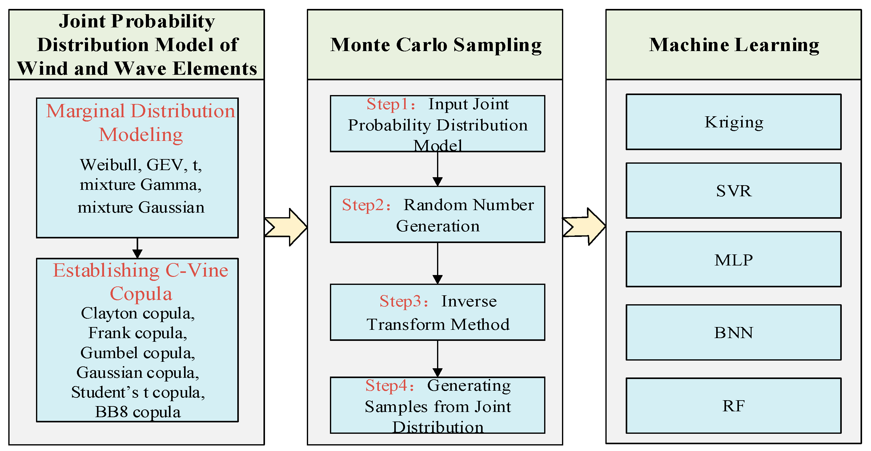
Figure 1. The schematic diagram of the methodology.
Jmse 12 01275 g001
Figure 2. Four-dimensional C-Vine Decomposition Structure.
Jmse 12 01275 g002
Figure 3. Block diagram of the multiphysics components involved in the FOWT simulation using OpenFAST.
Jmse 12 01275 g003
Figure 4. Framework of load modeling method for floating wind turbines.
Jmse 12 01275 g004
Figure 5. Structure of the NREL 5 MW OC4 Semi-Submersible Floating Wind Turbine. (a) The Structure of Semi-Submersible. Offshore Wind Turbine. (b) Arrangement of Mooring System Structure (①:Number 1 mooring line; ②:Number 2 mooring line; ③:Number 3 mooring line).
Jmse 12 01275 g005
Figure 6. Frequency histograms of sample data. (a) Frequency histogram and fitting curve of wind speed. (b) Frequency histogram and fitting curve of wind direction. (c) Frequency histogram and fitting curve of wave height. (d) Frequency histogram and fitting curve of wave period.
Jmse 12 01275 g006aJmse 12 01275 g006b
Figure 7. Marginal Distribution Results of Environmental Variables.
Jmse 12 01275 g007
Figure 8. C-Vine copula structure of wind and wave variables.
Jmse 12 01275 g008
Figure 9. Frequency histograms and optimal bivariate copula functions between wind and wave variables. (a) Frequency histogram of wind speed and direction. (b) PDF of wind speed and direction. (c) Frequency histogram of wind speed and wave height. (d) PDF of wind speed and wave height. (e) Frequency histogram of wave height and wave period. (f) PDF of wave height and wave period.
Jmse 12 01275 g009
Figure 10. Comparison between generated samples and original data. (a) Wind speed-wave height. (b) Wave height-wave period. (c) Wind speed-wind direction. (d) Wave height-wind direction.
Jmse 12 01275 g010
Figure 11. Frequency histogram of sampled wind and wave variables.
Jmse 12 01275 g011
Figure 12. Pearson correlation coefficients between environmental variables and DEL.
Jmse 12 01275 g012
Figure 13. Pearson correlation coefficients between operational state variables and DEL.
Jmse 12 01275 g013
Figure 14. Training results of the Kriging model.
Jmse 12 01275 g014
Figure 15. Training results of the MLP model.
Jmse 12 01275 g015
Figure 16. Training results of the SVR model.
Jmse 12 01275 g016
Figure 17. Training results of the BNN model.
Jmse 12 01275 g017
Figure 18. Training results of the RF model.
Jmse 12 01275 g018
Table 1. Parameters involved in the calculation of C-Vine copula and their descriptions.
ParameterDescription
f ( x 1 , x 2 , x 3 , x 4 ) the joint probability density function, x i is the random variable, i indicates the number of variables
c 1 i ( · , · ) , i = 2 , 3 , 4 , c 2 i | 1 ( · , · ) , i = 3 , 4 , c 34 | 12 ( · , · ) the bivariate copula density functions
F i the marginal cumulative distribution function of the random variable x i ( i = 1 , 2 , 3 , 4 )
F i | 1 , i = 2 , 3 , 4 , F i | 12 , i = 3 , 4 the conditional marginal distributions
f i the corresponding PDF of the random variable x i
Table 2. Parameters involved in the calculation of AIC and BIC and their descriptions.
ParameterDescription
x i the sample value
n the sample size
f ( x i ) the density function of the candidate marginal distribution function
k the number of distribution parameters in the candidate marginal distribution function
Table 3. Parameters involved in the calculation of RMSE and their descriptions.
ParameterDescription
n the sample size
P c the theoretical frequency value of the multidimensional copula joint distribution
P 0 the actual frequency value of the multidimensional copula joint distribution
k the number of distribution parameters in the candidate marginal distribution function
Table 4. Parameters involved in the calculation of BB8 copula and their descriptions.
ParameterDescription
u = F X ( x ) , υ = F Y ( y ) the cumulative distribution functions of random variables X and Y, respectively
θ a parameter controlling tail dependence, typically ranging within ( 0 , + )
δ a parameter controlling overall dependence strength, typically ranging within [ 1 , + )
Table 5. Parameters involved in the calculation of e and their descriptions.
ParameterDescription
T the theoretical values calculated by the established model
T ^ E the empirical values of the copula
nthe sample size, and for each 1 i n , I u 1 i u 1 , u 2 i u 2 = 1 when u 1 i u 1 , u 2 i u 2
Table 6. Parameters involved in the calculation of DEL and their descriptions.
ParameterDescription
f e q the frequency of the DEL
T j the time elapsed for time series j
n j S T e q the total equivalent fatigue counts for time series j
n j i the damage count for load cycle i in time series j
L j i R the range of load cycle i in time series j
ma Wöhler exponent
Table 7. Parameters and evaluation metrics of different marginal probability distribution models for wind speed, significant wave height, and wave period.
Environmental VariablesDistribution FunctionAICBICScale
Parameter
Shape
Parameter
Location
Parameter
RMSE
Wind SpeedWeibull153,586.8227153,603.42578.57322.38073 0.0092
GEV149,378.3867149,403.29122.353345.907680.1254760.0102
t155,712.173155,737.07752.852937.008712.852930.0130
Wave HeightWeibull−3994.0557−3977.49540.4286821.47096 0.2518
GEV−7216.5465−7191.70610.1508730.236530.336450.0915
t3109.94883134.78920.1710252.670720.3106430.1517
Wave PeriodWeibull127,452.0984127,468.70134.86592.33344 0.0408
GEV110,747.5038110,772.40831.534623.92278−0.0529920.0281
t99,020.190799,045.09510.9910974.155834.515040.0144
Gray represents the best fit distribution model for the environment variable.
Table 8. Parameters and evaluation metrics of different marginal probability distribution models for wind direction.
Environmental VariablesDistribution FunctionFitting ParametersRMSE
Wind DirectionMixed Gaussian ω 1 ω 2 ω 3 μ 1 μ 2 μ 3 σ 1 σ 2 σ 3 0.0021045
0.1605 0.25675 0.58275 31.5744 285.1857 122.6558 194.1401 1199.8808 1758.945
Mixed Gamma ω 1 ω 2 ω 3 μ 1 μ 2 μ 3 σ 1 σ 2 σ 3 0.0021123
0.18112 0.26093 0.55794 33.6104 284.1113 124.6439 243.2999 1258.9205 1550.5218
Gray represents the best fit distribution model for the environment variable.
Table 9. Empirical Kendall’s matrix and sum of Kendall’s tau.
VariablesWind SpeedWave HeightWave PeriodWind Directionτsum
Wind Speed10.4164370.0489680.1241231.589528
Wave Height0.41643710.0899140.3318071.838159
Wave Period0.0489680.08991410.0754821.214364
Wind Direction0.1241230.3318070.07548211.531413
Gray represents the variable with the highest correlation coefficient.
Table 10. Optimal bivariate copula functions for environmental variables.
Copula FunctionsParameter 1Parameter 2
Tree1 c 12 BB80.13638994 21.75006081
c 13 t0.58858094 6.73374776
c 14 t−0.4549795 7.68651773
Tree2 c 23 | 1 BB8−0.17235243 21.37793364
c 24 | 1 t0.0970424 13.29766572
Tree3 c 34 | 12 Gaussian−0.01858334
Table 11. Configuration and optimization methods of five machine learning models.
Machine Learning ModelsConfigurationOptimization
KrigingSet the kernel function type to RBF (Radial Basis Function)Genetic Algorithm
MLPTwo hidden layers with 8 and 12 neurons, respectivelyAdam Algorithm
SVRSet the kernel function to the Gaussian kernelSMO Algorithm
BNN4 neuronsBayesian Optimization
RFUsed a total of 200 decision trees with a leaf node size of 1K-fold Cross-Validation
Table 12. The MSE, RMSE, and R 2 of five machine learning models and the polynomial regression model.
Moment Kriging MLP SVR
MSERMSER2MSERMSER2MSERMSER2
RootMxb10.00550.07410.99390.25930.50920.71390.03880.19690.9571
RootMyb10.01770.13300.98040.10030.31670.88930.03110.17630.9656
RootMzb10.06190.24870.93170.17260.41540.80950.03340.18270.9631
TwrBsMxt0.01660.12880.98160.11860.34430.86910.04400.20970.9514
TwrBsMyt0.06190.24870.93170.11680.34170.87110.05570.23600.9385
TwrBsMzt0.02930.17110.96760.23040.48000.74570.02180.14760.9759
BNN RF Polynomial Regression
MSERMSER2MSERMSER2MSERMSER2
0.11920.34520.86840.00210.04580.99971.10941.05320.2240
0.23770.48750.73770.01320.11480.98541.35071.16210.4902
0.10930.33060.87940.02320.15230.97445.79642.40750.0952
0.39390.62760.56540.01260.11220.98603.60241.89790.0746
0.10140.31840.88810.03900.19740.95691.00221.00100.1057
0.12590.35480.86100.01170.10810.98701.67811.29540.1014
Gray represents the best data-driven model.
Disclaimer/Publisher’s Note: The statements, opinions and data contained in all publications are solely those of the individual author(s) and contributor(s) and not of MDPI and/or the editor(s). MDPI and/or the editor(s) disclaim responsibility for any injury to people or property resulting from any ideas, methods, instructions or products referred to in the content.