Abstract
Submerged tensioned anchor cables (STACs) are pivotal components utilized extensively for anchoring and supporting offshore floating structures. Unlike tensioned cables in air, STACs exhibit distinctive nonlinear damping characteristics. Although existing studies on the free vibration response and tension identification of STACs often employ conventional Galerkin and average methods, the effect of the quadratic damping coefficient (QDC) on the vibration frequency remains unquantified. This paper re-examines the effect of bending stiffness on the static equilibrium configuration of STACs, and establishes the in-plane transverse free motion equations considering bending stiffness, sag, and hydrodynamic force. By introducing the bending stiffness influence coefficient and the Irvine parameter, the exact analytical solutions of symmetric and antisymmetric frequencies and modal shapes of STACs are derived. An improved Galerkin method is proposed to discretize the nonlinear free motion equations ensuring the accuracy and applicability of the analytical results. Additionally, this paper presents an analytical solution for the nonlinear free vibration response of the STACs using the improved averaging method, along with improved frequency formulas and tension identification methods considering the QDC. Through a case study, it is demonstrated that the improved methods introduced in this paper offer higher accuracy and wider applicability compared to the conventional approaches. These findings provide theoretical guidance and reference for the precise dynamic analysis, monitoring, and evaluation of marine anchor cable structures.
1. Introduction
The submerged tensioned anchor cable (STAC) [1,2] is an important tension component connecting the foundation and platform in marine infrastructure, such as offshore floating oil and gas production platforms [3,4,5], floating wind turbines [6,7,8,9], floating bridges [10,11], and floating tunnels [12]. The bearing capacity of the STAC will directly determine the safety of the entire marine structure. Given its lightweight, high tension strength, and low damping properties, STACs are prone to large-scale nonlinear vibrations under complex environmental loads like waves and currents. Therefore, accurately understanding the STAC’s dynamic behavior is of great engineering significance to ensure the safe operation of both the STAC structure and the entire platform system [1,2,13,14,15,16,17].
At present, the common dynamic models of the STACs include the spring model [13,18], lumped mass model [19,20], multi-body dynamics model [21,22], taut string model [23,24], and three-dimensional finite element model [25,26]. These models have certain feasibility in studying the overall dynamic characteristics of the floating platform system. While a three-dimensional finite element model offers precise calculations, its efficiency is often insufficient for practical engineering applications. On the other hand, the tensioned string model, commonly employed, oversimplifies the problem by neglecting factors such as bending stiffness and sag, hindering refined dynamic analysis of the STACs. In fact, as a unidirectional tensile flexible structure, STACs offer a particular sag under the action of buoyancy, self-weight, and axial force. Therefore, considering the sag of STACs to determine its initial configuration can reduce the error caused by the sag effect of STACs in static and dynamic analysis [15,27,28]. Since STACs possess a certain bending stiffness, especially when the length is short or the diameter is large, the effect of the bending stiffness on the structure’s static/dynamic characteristics cannot be ignored [29,30,31]. At the same time, the nonlinearity of hydrodynamic resistance significantly affects the vibration characteristics of the STACs, which makes the vibration characteristics of the STACs substantially different from that of tensioned cable in air [32]. In addition, it has been shown that the out-of-plane motion can be neglected when calculating the response of submerged slender structures [33,34]. Therefore, to fully consider the effect of factors such as the bending stiffness, sag, and damping of the STACs, Han et al. [1,2] adopted the Euler beam model considering the axial tension, which provided an idea for the fine nonlinear dynamic theoretical modeling of the STACs.
In the process of discretizing the dynamic model of the STACs, the rationality of the modal function selection will directly affect the accuracy of the calculation results. Compared with air bridge cables, STACs face a more complex marine environment, where their diameters and bending stiffnesses may be larger and their lengths may be smaller. The effects of sag, axial force, and bending stiffness on the static/dynamic characteristics of the STACs are more pronounced. So far, there are few studies that consider the effects of both sag and bending stiffness in the analysis of modal characteristics of the STACs. The conventional Galerkin discretization method uses the modal shape of string or simply supported beam as the shape function [14,15], or the analytical model of modal shape, considering bending stiffness but ignoring the effect of sag [1]. In some cable structures with large initial tension in practical engineering, the sine function model is still favored due to its elegant and convenient mathematical properties. However, the defects are also obvious, and even the calculated frequency values are inaccurate within a certain parameter range, e.g., for anchor cable structures with small initial tensions, short lengths, or thick diameters. Therefore, it is necessary to use more accurate modal eigenfunctions in the analytical calculation of the natural frequency of the STACs and the discretization of the partial differential equation to avoid unnecessary errors in the calculation process. This implied precondition highlights the constraints of the conventional Galerkin method in accurately determining the modal characteristics and vibration response of anchor cable structures. Furthermore, the study indicates that when the effects of bending stiffness and sag on the modal characteristics of the STACs are substantial and cannot be overlooked, the analytical solution presented in this paper offers a more precise and practical alternative.
Due to the complexity of the nonlinear motion equation of the STACs, it is generally challenging to derive its exact solution, so an approximate analytical method can be adopted to solve it. The commonly used analytical methods mainly include the following [35]: progressive method, harmonic balance method, Lindstedt–Poincare (L-P) method, multi-scale method, averaging method, etc. Although the averaging method has low accuracy in the above methods, it can avoid complicated intermediate operations and has outstanding advantages in convenient application. Han et al. [1,2] derived the approximate analytical solution of the free vibration response of the STACs using the averaging method based on the assumption of weak nonlinearity in the system. When the averaging method is used to solve the free vibration equation of the STACs, whether linear damping or nonlinear hydrodynamic damping, the averaging method has higher accuracy when the damping coefficient is small [2,17]. However, as the quadratic damping coefficient (QDC) increases, its influence on the vibration frequency will gradually increase. At this time, the results of the averaging method solution deviate from the numerical exact solution, which is also proven in the case study later. Therefore, the improved averaging method [36,37] is introduced in this paper to derive the approximate analytical solution of the nonlinear free vibration response of the STACs.
In the process of deducing the free vibration response of the STACs based on the improved averaging method, not only the effect of QDC on the vibration frequency can be investigated, but also the tension characteristics can be further studied. As is known to all, as an essential stress component of offshore floating platforms, STACs aggravate their fatigue and fracture due to their vulnerability to vibration and corrosion, affecting the safety of the entire platform system [38,39,40]. Therefore, accurately identified cable tension is of great significance for safety monitoring and condition assessment of floating platforms moored with STACs. The existing cable tension identification methods include the direct method and the indirect method. The direct method refers to the direct measurement of cable tension, including the jack tension method, sensor reading method, and pressure gauge measurement method. It is difficult to measure cable tension directly in a marine environment due to the limitation of test conditions. The indirect method identifies the cable tension by measuring indirect physical quantities, including the magnetic flux method, sag method, and vibration frequency method. Similar to the tensioned cable in the air, the vibration frequency method is widely used because of its low cost, simplicity, and high efficiency [17,41,42]. The basic principle of this method is to first identify the vibration frequency of the cable structure through the structural response signal, then indirectly calculate the cable tension according to the functional relationship between the cable tension and the vibration frequency. The accuracy of identified cable tension based on the vibration frequency method is affected by many factors, such as the cable’s bending stiffness, sag, inclination angle, and boundary conditions [17,41,42,43,44,45,46]. However, the effect of QDC on the accuracy of identified cable tension is not quantitatively considered in the above studies. In fact, the drag coefficient on the surface of different STACs will affect the size of its QDC, which in turn affects the vibration frequency and may ultimately affect the results of identified cable tension.
In summary, this paper aims to refine analytical methods for determining the natural vibration characteristics and cable tension of the STACs, providing a more accurate and practical approach for analyzing modal characteristics, free vibration response, and cable tension values. Bending stiffness is factored into both the static equilibrium and motion equations of the STAC, while the nonlinear free motion equation considers bending stiffness, sag, and damping. By introducing the non-dimensional bending stiffness influence coefficient and Irvine parameter, the exact analytical models for in-plane symmetric and antisymmetric frequencies and modal shapes are derived. In Section 2, an improved Galerkin method is introduced, employing the exact modal shape functions to discretize the nonlinear free motion equation for STAC, departing from the conventional standard sine function. Section 3 presents the derivation of an approximate analytical solution for the nonlinear free vibration response of the STAC utilizing the improved average method. Additionally, it outlines the analytical calculation method for the STAC’s frequency, incorporating the influence of the QDC. Section 4 introduces an improved method for identifying cable tension based on vibration frequency, considering both the exact frequency and QDC. Section 5 analyzes and verifies these theories using a typical floating structure mooring cable as an example. The above related studies contribute to addressing the limitations of the existing theories in finely analyzing the dynamic characteristics of the STACs. Additionally, they serve as a valuable theoretical resource for the engineering application, monitoring, and evaluation of marine anchor cables.
2. Improved Analytical Model for Free Vibration Characteristics of STACs
Figure 1 shows the mechanical model of a STAC hinged at both ends. O is the coordinate origin, OP is the longitudinal x-axis, and the direction perpendicular to the x-axis is the transverse y-axis. The positive direction is as shown in Figure 1. The symbols in the figure represent the elastic modulus, moment of inertia, per length mass, cross-sectional area, chordwise initial cable tension, mid-span sag, and chordwise length of the STAC, respectively. is the angle between the STAC and the horizontal line under static state. , denote the STAC’s initial configuration and in-plane lateral vibration displacement, respectively.
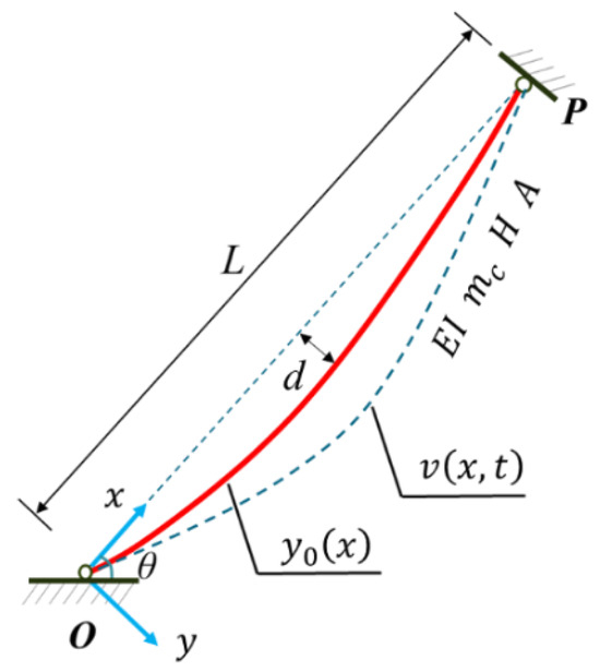
Figure 1.
Mechanical modeling of STAC.
2.1. Static Equilibrium Equation
When the ratio of the mid-span sag d to the chord length L is , then the static equilibrium equation of the STAC considering the self-weight and bending stiffness of the cable structure is as follows [47]:
where , , is the wet density of the STAC, , is the density of the anchor cable in air, is the density of seawater, g is the acceleration of gravity, D is the outer diameter of the STAC, and is the initial chordwise cable tension.
Assuming that the STAC is hinged at both ends, the exact non-dimensional solution of in Equation (1) can be obtained as follows:
where , , denotes the effect coefficient of bending stiffness, which can control the relative importance of the cable–beam action [29,43,48].
2.2. Dynamic Motion Equation
Assuming that the STAC moves only in the xy plane, the in-plane transverse free vibration equation in Figure 1 is as follows [1,27,28]:
where is the bending stiffness, ; denotes the viscous damping coefficient of the STAC; is the chordwise tension increment during the STAC vibration, which is assumed to be a function of time t only. According to the deformation compatibility equation of elastic cable, the yields the following [27]:
where is the axial stiffness. is the total length of STAC in static state. The STAC can be regarded as a flexible structure with a large slender ratio. in Equation (3) is the hydrodynamic force per unit length generated by the movement of the STAC in the y-axis direction, consisting of the sum of the additional inertial force and the water-body damping force, which can be calculated by the Morison’s equation [49]:
where is the additional mass coefficient, in this paper. is the drag force coefficient, reflecting the viscous effect caused by the viscosity of the fluid, which is related to the Reynolds number and the surface roughness of the cylinder [50].
In summary, the partial differential equation of in-plane transverse free vibration of the STAC can be further expressed as:
where , .
2.3. Exact Frequencies and Modal Shapes Considering Bending Stiffness and Sag
This study proposes a cable–beam model with two non-dimensional parameters (the effect coefficient of bending stiffness) and (Irvine parameter [27]) to characterize the exact frequencies and modal shapes of the STAC, and its initial configuration is chosen to consider the effects of in Equation (2). In the case of the antisymmetric mode, is an odd function about x, and is zero in the symmetric integral interval, at this time, . Only in the case of symmetric mode, .
2.3.1. Antisymmetric Mode
For the case of in-plane antisymmetric mode, in Equation (6). Then, let , the undamped free vibration equation of the STAC is expressed as
where .
By using the method of separation of variables, let () and substitute it into Equation (7) to yield
where and represent the eigenfrequencies and modal shapes, respectively. The can be solved from Equation (8) [28,41]:
where are constants determined by the initial conditions; and are calculated as
Introducing non-dimensional parameters , , and substituting into Equation (10) yields
The analytical solution of natural frequency and modal shape of the exact antisymmetric mode in the simply supported STAC at both ends is derived from the non-dimensional boundary conditions , , namely:
where are non-zero constants.
2.3.2. Symmetric Mode
For the case of in-plane symmetric mode, in Equation (6), and then the undamped free vibration equation of the STAC is
Setting , , and substituting Equation (2) into Equation (4) obtains
Substituting Equation (2) and into Equation (14) yields
Introducing the non-dimensional parameter , the analytical solution to the non-dimensional form of Equation (16) is
where are constants, .
Non-dimensional boundary conditions for the STAC with simply supported ends are , , and the non-dimensional modal shape function of the exact symmetric mode is obtained as
Substituting Equation (18) into Equation (15), the exact natural frequency of the STAC can be derived:
From the analytical solution of the frequencies of the Equations (12) and (19), it can be found that and determine the frequency of the STAC, while and are related to the sag and bending stiffness, respectively, where can control the STAC to move like a beam or a cable.
When , the STAC can be regarded as an Euler–Bernoulli beam, and its symmetrical modal frequency is expressed as
At this time, the corresponding non-dimensional modal shape function of the STAC is , where are non-zero constants.
When , the STAC can be considered as a sagging cable without considering the bending stiffness, and its symmetrical modal frequency can be expressed as
where
Equation (21) is the transcendental equation of the natural frequency of the small sag cable without considering the bending stiffness, which was first proposed by Irvine and Caughey [51].
When , it can be obtained from Equation (21):
Solving Equation (23) yields [27]
When , at this time, , the deflection of the STAC tends to zero, which can be regarded as a taut string. From Equation (21), it can be obtained as follows:
Solving Equation (25) gives
The deviation of in Equations (24) and (26) is approximately for both limit conditions.
The above derivation reveals that both the beam model and the cable model, as well as the string model, are merely specific cases of the more comprehensive cable–beam model described by Equations (18) and (19) in this paper. Theoretically, the cable–beam model presented herein offers higher accuracy and broader applicability across non-dimensional parameters and .
2.4. Modal Discretization Based on Galerkin Method
Given the nonlinear term of damping force in the partial differential Equation (6) describing the in-plane transverse vibration of the STAC, it is customary to employ variable separation followed by discretization into an ordinary differential equation using the Galerkin method. Consequently, the displacement of the STAC can be represented as follows:
where is the generalized coordinate that responds to the n-th modal amplitude. is the n-th order modal shape. Substituting Equation (27) into Equation (6), n-th order ordinary differential equations about can be obtained by utilizing the orthogonality of the modal shapes. Therefore, we can find that a reasonable choice of the mode shape function in Equation (27) will directly affect the accuracy of the dynamic analysis results. This paper proposed an improved Galerkin method aimed at ensuring the accuracy of the subsequent analyses concerning free vibration response and cable tension identification. For clarity, the conventional Galerkin method and the improved Galerkin method based on the cable–beam model suggested in this paper will be presented in Section 2.4.1 and Section 2.4.2, respectively.
2.4.1. Conventional Galerkin Method Using Standard Sine Shapes
In the conventional method to the study of the in-plane transverse vibration response characteristics of the STAC, the modal shape function is mostly represented by the normalized n-th order standard sine shapes, that is:
Substituting Equations (27) and (28) into Equation (6), the initial configuration of the STAC is described by a parabola, namely , and the Galerkin method is used to transform the partial differential equation into differential equation:
where
where denotes the sign function; N represents the number of modes.
The value of n in Equations (29) and (30) will directly affect the number of ordinary differentials and the efficiency of the solution. Therefore, based on the Galerkin method, the value of n usually does not exceed three, then Equation (29) can be further summarized as
where , , , , , is the n-th natural frequency of the STAC with simply supported ends considering the effect of bending stiffness, that is:
Furthermore, the n-th order natural frequency of the STAC utilizing the conventional Galerkin method and considering the effects of sag and bending stiffness can be obtained as
2.4.2. Improved Galerkin Method Using Exact Modal Shapes
According to the analytical solution of the exact modal characteristics of the STAC system, it is assumed that the in-plane transverse vibration of the STAC is a multi-degree-of-freedom system consisting of antisymmetric modes and symmetric modes. In this subsection, the improved Galerkin method is proposed to discretize Equation (5) by using the modal shapes of Equations (13) and (18), assuming that the in-plane transverse vibration displacement of the STAC can be expressed as
where is the n-th order mode shape function, which can be obtained by eliminating the lack of dimension of Equations (18) and (13), respectively, namely:
Symmetric modal shapes:
Antisymmetric modal shapes:
where is the amplitude of the n-th order modal vibration of the STAC.
Substituting Equation (34) into Equation (6), multiplying the terms at both sides of Equation (6) by , integrating them in , and considering the orthogonality of modal shapes, then the cable–beam model based on the exact modal shapes of this paper, and the discrete model using the improved Galerkin method is
where is calculated from Equations (17) and (24), , , , the QDC is
It can be seen from Equation (38) that the QDC is proportional to the drag coefficient when the outer diameter D of the STAC is determined.
3. Analytical Solution for Free Vibration Response Based on Improved Averaging Method
Due to the existence of hydrodynamic damping force, the system energy will decay rapidly under the initial conditions and eventually reach static equilibrium. When and are very small (), they are regarded as small parameters, and Equation (37) can be solved by weak nonlinear vibration approximation methods such as the averaging method [1,2,17,52]. However, for the vibration problem of the STAC, according to Equation (38), it can be found that is positively correlated with the drag force coefficient . When can no longer be regarded as a small parameter, not only attenuates the amplitude of free vibration but also affects the frequency of damped vibration. In view of this, this paper adopts the improved averaging method [36,37] to solve the approximate analytical solution of free vibration response of the STAC.
The standard nonlinear differential equation of motion that Equation (37) can be written as is as follows:
where
Comparing Equations (37) and (39), it can be seen that . The derived system equation of Equation (39) is , and its solution is . Let the solution of Equation (39) be of the same form as the solution of the derived equations, but the amplitude and initial phase change slowly with time. The difference between the improved averaging method and the conventional averaging method is that the vibration frequency of the solution of Equation (39) is , which changes with the damping coefficient rather than in the solution of the derived system. That is as follows:
Let , , and in the above equation can be determined by Equations (41) and (42), and the boundary conditions, then:
where F is called the difference function, which reflects the change in frequency of the STAC system from to , caused by damping and other factors, expressed as
is determined by the damping coefficient with the term in Equation (39), and it is usually only necessary to use the coefficients directly in front of the term as F, which gives a high accuracy in many practical problems [36].
When the difference between and is not large, it can be obtained according to Equation (45) and Taylor’s expansion formula, and taking the first three terms:
Since the damping ratio of the STAC is small, for the convenience of calculation, is taken in this paper, and then it can be obtained from Equations (43) and (44):
where and are the initial amplitude and initial phase, respectively. Let the initial conditions , and substitute into Equations (41) and (42) can be calculated:
According to the frequency calculated by Equations (12) and (19), and combined with Equation (46), the improved frequency can be calculated as
Equation (49) can quantitatively consider the effect of the QDC on the vibration frequency of the STAC. Substituting Equations (47)–(49) into Equation (41), the approximate analytical solution of Equation (37) calculated by the improved averaging method can be obtained as follows:
Equation (50) reflects the law of free vibration of the STAC in water, and the amplitude attenuation is non-exponential. In order to facilitate the comparison of the difference between the improved averaging method and the averaging method for calculating the free vibration response of the STAC, the main results of the two methods are also outlined in Table 1. In this paper, the approximate analytical solution of the free vibration of the STAC based on the improved averaging method has advantages over the results in Refs. [1,2,17]:

Table 1.
Outline of the main results of the averaging method and improved averaging method for calculating the free vibration response of the STAC.
(1) The improved averaging method is no longer restricted to weakly nonlinear systems and has wider applicability to solve the free vibration response of the STACs.
(2) The effect of QDC on the vibration frequency of the STACs and the cable tension identification results can be quantitatively considered.
4. Improved Tension Identification Method Considering QDC
Most of the existing cable tension identification methods for the STACs are derived based on the conventional Galerkin method, which ignores the effect of the QDC on the vibration frequency, despite accounting for the effects of bending stiffness and sag on the frequency [17]. To address this, this section firstly lists the conventional tension identification formula, considering either the effect of bending stiffness or the combined effect of bending stiffness and sag. Subsequently, based on the exact characteristics of the STAC (cable–beam model) in this paper, the improved tension identification method considering the effect of the QDC is given. Traditionally, the conventional tension identification formula based on the vibration frequency method is obtained from Equation (37) [41]:
where is the n-th order undamped natural frequency of Euler beam.
In order to consider the effect of sag on the cable tension identification by the vibration frequency method, Han and Duan [17] gave the modified tension identification formula considering the effect of sag based on Equation (51), that is:
Equations (51) and (52) are the cable tension identification formulas based on the Euler beam model and the modified formulas after considering the effect of sag, respectively. As mentioned in Section 2.4.1, there are some limitations in their accuracy and applicability for specific anchor cable structures. Therefore, based on the exact modal characteristic equation of the STAC given in this paper, i.e., the cable–beam model, the cable tension identification formulas with higher accuracy and more general applicability are given as follows:
(1) When the modal order n is even, the tension identification formula can be determined by the analytical solution of the antisymmetric frequency (Equation (12)), which is similar to Equation (51):
(2) When the modal order n is odd, the tension identification formula can be calculated by the analytical solution of the symmetric frequency (Equation (19)), which can be written as:
In Equations (53) and (54), the parameters are known for a specific STAC, so the relationship between the frequency and H can be established. When the tension H is a known physical parameter, the frequency can be calculated by the corresponding formula in Section 2.3. When the tension H is unknown, the frequency can be calculated by the corresponding dynamic response, which is an inverse problem of dynamics. Therefore, once the frequency is calculated from the dynamic response of the STAC, the tension H can be identified by the vibration frequency method. It should be noted that Equation (19) is a complex implicit function; the Newton iteration method will be used to estimate the value of tension H in this paper.
In fact, due to the effect of hydrodynamic damping force and additional mass, the mechanical environment of the STACs is essentially different from that of cables in the air. Although Equations (53) and (54) consider the effect of additional mass, neither of them quantitatively considers the effect of the QDC on the vibration frequency of the STAC, and the sensitivity of to tension identification deserves to be further explored. In view of this, this paper improves in Equations (53) and (54) according to in Equation (49), and the steps of the improved tension identification method are summarized as follows:
(1) Fast Fourier transform (FFT) is performed on the dynamic response time histories of the STAC considering the hydrodynamic damping force, and its frequency is obtained.
(2) The improved frequency is calculated by substituting into Equation (49), and an estimated tension value can be obtained by using to replace in Equation (51).
(3) Substituting into the Equations (53) and (54), and taking as the initial value for calculating Equation (54), the cable tension H of the STAC can be identified via the improved method.
5. Case Study
For the same STAC, different initial tensions H cause different Irvine parameters , and also affect the parameters . Therefore, the values of the initial tensions in this paper are given in the specific calculations (all satisfy ), and the other basic parameters about a typical floating structure mooring anchor cable are shown in Table 2 [1].
Table 2.
STAC’s parameters.
In order to ensure the reliability and applicability of the theoretical results, the results of the exact modal characteristics of this paper are compared with the other literature results in Section 5.1. In Section 5.2, the exact frequencies (Equation (19)), the frequencies obtained via the traditional Galerkin method (Equation (33)), and the finite element (FE) results are investigated, and the numerical solution via two discretization methods and FE solutions of displacement responses are further analyzed. Subsequently, in Section 5.3, we analyze the differences between the analytical solutions of the free vibration displacement response of the STAC based on the improved average method, and the average method and numerical results under different quadratic damping coefficients (or drag force coefficients). Section 5.4 quantitatively compares the effects of different quadratic damping coefficients on the vibration frequency of the STAC. Finally, the analytical formulas for in-plane free vibration frequency considering the effects of sag, bending stiffness, and quadratic damping coefficient are applied to the cable tension identification of the STAC in Section 5.5.
5.1. Analysis of Modal Characteristics
This section mainly discusses the effect of non-dimensional parameters and on the modal characteristics of the STACs.
5.1.1. Effect of Non-Dimensional Parameters on Antisymmetric Modes
In this section, the relationship between the non-dimensional frequency of the antisymmetric mode of the STAC and and is studied. Irvine [27] gave the n-th order natural frequency of the string without considering the bending stiffness:
The natural frequency of the STAC is normalized with respect to the first mode frequency of the tensioned string. The purpose is to obtain a curve similar to that in Irvine [27], that is:
where , .
It can be seen from Figure 2 that the in-plane antisymmetric modal frequency of the STAC is independent to (sag) (Note: and in Equation (56) in this paper are uniformly represented by in the figure). According to Figure 2a and Table 3, it can be found that in order to ignore the effect of bending stiffness on the first-order antisymmetric modal frequency of simply supported anchor cables at both ends, it is necessary to make , at which time . According to Figure 2b and Table 3, when , then the effect of bending stiffness on the second-order antisymmetric frequency of the STAC can be ignored. Therefore, it can be found that for the higher order in-plane antisymmetric modal frequency, a larger value of is needed to ignore the effect of the bending stiffness. In addition, the first two orders of antisymmetric modal shapes are obtained according to Equation (13) as shown in Figure 3, and they are only related to the mode order, but not to the non-dimensional parameters and .
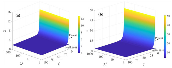
Figure 2.
Non-dimensional frequency of first two antisymmetric modes versus non-dimensional parameters and : (a) 1st order frequency; (b) 2nd order frequency. Irvine, 1981 [27].
Table 3.
Non-dimensional frequency of antisymmetric modes .
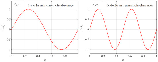
Figure 3.
First two orders of antisymmetric modal shapes.
5.1.2. Effect of Non-Dimensional Parameters on Symmetric Modes
Considering the expression of non-dimensional frequency of in-plane symmetric vibration affected by and as a complex transcendental equation, it is difficult to solve the roots of the equation directly. Therefore, this paper adopts the Newton iteration method to solve Equation (19), and obtains the non-dimensional frequencies under some typical parameters as shown in Table 4. When (or ), the value of the first two orders of non-dimensional frequencies are approximately calculated by in Equation (20). At this time, the STAC is similar to the Euler–Bernoulli beam, and the effect of on the natural frequency can be ignored. When , from Equation (19) and Equation (56), the value of is the same as the result obtained from in Equation (21) [27]. With the increase of , the first-order frequency increases from 1 to 2.86, and the second-order frequency from 3 to 4.920, which corresponds to the change from the string model to the cable model that does not take into account the bending stiffness [27]. When , the maximum relative errors between the first two order frequencies and the calculation results of Irvine [27] are 4.96%, 1.97%, and 1.26%, respectively, which are within the engineering tolerance of 5%. Therefore, it can be considered that when , the anchor cable can be regarded as a cable structure without considering the bending stiffness, and the effect of on its natural frequency can be ignored. When decreases gradually, its effect on the in-plane symmetrical frequencies becomes gradually larger. For example, when , the first-order symmetrical frequency increases from 1.045 to 4.003, and the second-order symmetrical frequency increases from 4.120 to 9.257, which is completely different from the calculation results of Irvine [27] that the symmetrical frequencies increase to 2.86 (first order) and 4.920 (second order), respectively. At this time, the modal characteristics of the STAC are intermediate between those of the cable–beam. Similarly, the modal characteristics at and are also between the cable and beam, except that as decreases, has a greater effect on the vibration of the STAC than . At this time, the value of converges to a higher order until the vibration of the STAC resembles that of an Euler–Bernoulli beam (i.e., ).
Table 4.
Non-dimensional symmetric frequency .
Figure 4 shows the first-order non-dimensional symmetric modal shapes corresponding to different values of at , which are calculated by the modal shapes given in this paper (Equation (18)), those proposed by Irvine [27], and those computed by the beam or string theory models, respectively. The parameters in Figure 4a–d are 1, 5, 10, and 28, respectively. Since the modal shapes proposed by Irvine [27] and those calculated by beam or string theory models are not affected by (blue dashed and black dotted lines in the figure, respectively), the shapes of these two modal shapes remain unchanged in Figure 4, whereas the modal shapes given in this paper change with (red solid lines). When is small, as in Figure 4a at , the modal shape given in this paper is very close to that of the beam or string. When , as in Figure 4b, there is a big difference between the three modal shapes. It can be found from Figure 4c,d that, with the increase of , the difference between the modal shape given in this paper and the modal shape proposed by Irvine [27] gradually decreases, and it almost matches exactly at . At this time, the modal shapes are closer to the cable structure without considering the bending stiffness. The analysis based on the modal shape perspective (Figure 4) is consistent with the analysis based on the modal frequency perspective (Table 4).
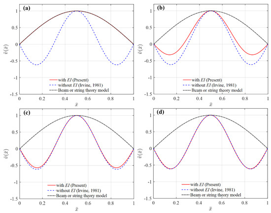
Figure 4.
First-order symmetric modal shapes corresponding to different models and values of at : (a) , (b) , (c) , (d) . Irvine, 1981 [27].
For the cable structures of practical engineering, such as STAC (inclined tension leg) [1], main cable of suspension bridge or cable-stayed bridge [48], high-voltage transmission line [53], etc., researchers can calculate the values of and according to the basic parameters of the cable structures. After making judgments according to the ideas given in this paper (e.g., Table 4 and Figure 4), they can then choose a more concise and accurate expression of modal characteristics. In addition, it can be seen from Equation (18) that the symmetric modal shapes are a function of non-dimensional parameters and . In this paper, the first two orders of symmetric modal shapes are given for different cases of and , as shown in Figure 5 and Figure 6. Figure 5 shows the first-order symmetric modal shapes for different values of when , , , , and Figure 6 is the corresponding second-order symmetric modal shapes. It can be observed that, with the change in and , the first two orders of symmetric modal characteristics are similar to the analytical results of Table 4 and Figure 4, which are not repeated here.
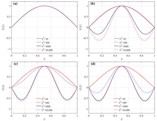
Figure 5.
First-order symmetric modal shapes for different and cases: (a) , (b) , (c) , (d) .
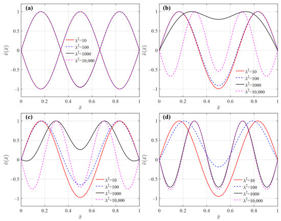
Figure 6.
Second-order symmetric modal shapes for different and cases: (a) , (b) , (c) , (d) .
5.2. Comparison of Discretization Methods
5.2.1. Comparison of Natural Frequency
According to the basic parameters in Table 2, the relationship between the non-dimensional parameters and of the STAC and H is shown in Figure 7. It can be seen from Figure 7 that when other parameters of the STAC are determined, the bending stiffness coefficient increases with the increase of H, and decreases rapidly with the increase of H and approaches zero.
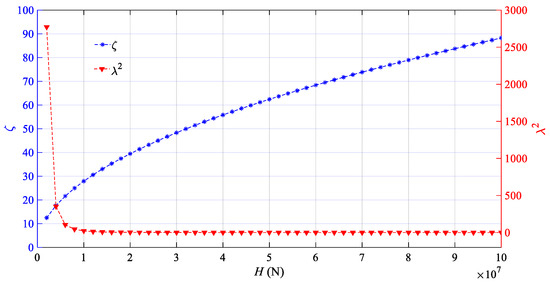
Figure 7.
The relationship between non-dimensional parameters and of the STAC and H (: blue line; : red line).
Combined with the non-dimensional parameters and in Figure 7, Table 5 compares the analytical solution of the symmetric modal frequencies of the STAC with the finite element (FE) results. The first two order frequencies given by the cable–beam model (Equation (19), n = 1, 3 in Table 5) and the conventional Galerkin method (Equation (33), n = 1, 3 in Table 4) and the frequency values calculated by the finite element method (FEM) [29] are compared. As can be seen from Table 5, the results of the cable–beam model given in this paper are basically consistent with those of the FEM. However, it is noteworthy that as the initial tension H decreases, there is a tendency for relative errors between the two methods to increase, albeit remaining within an overall range of 4%.This trend arises due to the neglect of higher order micro-quantities in the dynamic tension increment and the higher order term during the formation of the equations of motion in Section 2.2, and the nonlinear effects caused by these high order terms will be amplified with the decrease in H [54].
Table 5.
Comparison of symmetric modal frequencies of STAC with FE results.
The nonlinear effects stemming from these higher-order terms become more pronounced with decreasing H. Specifically, when the initial tension is high (), the relative error between the conventional Galerkin method and FEM results remains below 5%. However, as H gradually decreases (), the error in frequencies escalates rapidly, with the relative error of the first-order frequency even reaching 333.02% when . Consequently, it becomes evidently untenable to employ the conventional Galerkin method for calculating the natural frequency of the STAC under such conditions.
It is worth noting that as H gradually increases (e.g., , in Table 5), increases and decreases. In this case, the cable–beam model and the conventional Galerkin method can accurately calculate the symmetric modal frequency, because the parameters and have limited effect on the modal characteristics of the STAC, and its modal characteristics are similar to those of the beam or string, which is consistent with the analytical results in Section 5.1. At this time, the conventional Galerkin method can be used to calculate the natural frequency of the STAC from the perspective of the convenience and efficiency of the calculation for engineering applications.
5.2.2. Comparison of Displacement Response
In order to facilitate the study, this section only considers the first-order symmetric mode. So that n = 1 in Equations (31) and (37), and the in-plane first-order symmetric free vibration response of the STAC is calculated by using the Runge–Kutta method and with the help of mathematical software MATLAB R2018b. The basic parameters of the STAC are shown in Table 2, and the drag force coefficient is taken as . Combined with Table 5, the initial tensions are taken as , , , and , respectively, to show the difference between the response results calculated by the improved Galerkin method and the conventional Galerkin method. It should be noted that the frequency units in Equations (31) and (37) are rad/s. With the initial conditions of and , Figure 8 shows the displacement time histories of the two models (Equations (31) and (37)) at . It can be seen that the results obtained by the improved Galerkin method and the FEM are always in better agreement with the change in the initial tension H. Comparing the displacement time histories obtained by the traditional Galerkin method and the improved Galerkin method, the larger the initial tension H is, the better the displacement time history of the two models coincide (e.g., Figure 8d). When (Figure 8b) and (Figure 8c), although the trend of the results obtained by the two models is roughly the same, the quantitative difference between the results is also obvious. And when the initial tension H is small (e.g., Figure 8a), the displacement time histories and natural frequencies between the two models are quite different. This is similar to the comparative analysis results of the analytical frequency in Section 5.2.1, which further proves the limitations of the conventional Galerkin method in the vibration response analysis of the STAC.
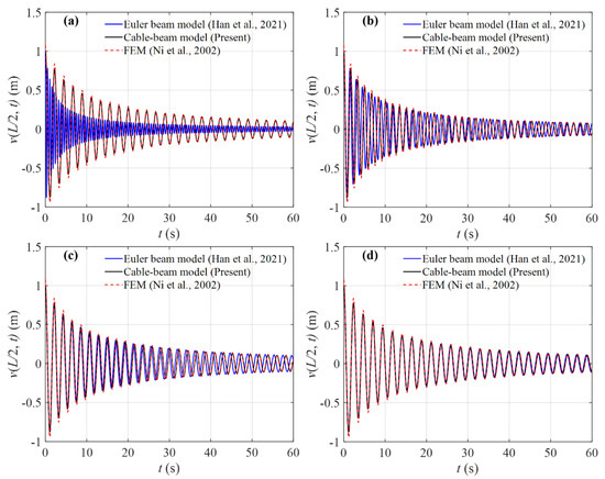
Figure 8.
Comparison of displacement time history at for three models: (a) , (b) , (c) , (d) . Han et al., 2021 [1], Ni et al., 2002 [29].
5.3. Verification of Free Vibration Response
In order to better verify the accuracy of the analytical method for the free vibration response of the STAC, the Runge–Kutta method is applied to solve Equation (37) numerically in MATLAB R2018b to obtain the exact solution of the vibration response in this paper. For ease of use, the DNV specification [50] recommends a range of values for the drag coefficient for different roughness cases from 0.5 to 1.2. According to the basic parameters in Table 2 and taking the drag coefficients as 0.5, 0.7, 0.9, and 1.1, the corresponding QDCs are calculated according to Equation (38), which are 0.0738, 0.1033, 0.1328, and 0.1623, respectively. Taking n = 3, , and the initial conditions are and , the time history results of the free vibration response of the STAC based on the improved averaging method (present method), the averaging method [1,2] and the numerical method can be obtained, as shown in Figure 9.
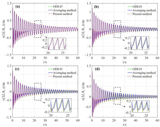
Figure 9.
Comparison of displacement response time history calculated by three methods. (a) ; (b) ; (c) ; (d) .
It can be found in Figure 9 that the three methods are in good agreement when the QDCs are small. However, with the increase of QDCs, the analytical results obtained by the improved averaging method proposed in this paper are in better agreement with the numerical exact solutions. In contrast, the accuracy of the analytical results obtained by the averaging method gradually deteriorates with the increase in . Similar results can also be found in Table 6. When , the maximum relative error (maximum difference/maximum displacement) between the free vibration displacement of the STAC calculated by the averaging method and the numerical accurate solution is 12.18%, which is almost twice that of the improved averaging method (6.56%). The main reason for the above results is that the QDC is proportional to the drag coefficient . As increases, can no longer be considered as a small parameter. At this time, not only affects the amplitude of free vibration but also affects the frequency of free vibration of the STAC to some extent. It can be seen that the improved averaging method can more accurately describe the response characteristics of the free vibration of the STAC and has a wider application range.
Table 6.
The maximum relative error between the displacement response calculated by different analytical methods and the exact numerical solution.
In order to estimate the numerical solution of vibration frequency and damping ratio of the STAC, is taken as an example. Firstly, the free vibration response of the anchor cable in hydrostatic water and air is calculated using the Runge–Kutta method, as shown in Figure 10a and Figure 11a. Then, the vibration frequency of the displacement response of the anchor cable at is obtained by fast Fourier transform (FFT), as in Figure 10b and Figure 11b. The damping ratio can be calculated by Equation (57) as follows:
where , are expressed as the peak value of the displacement response of the anchor cable decreases from to after i damping cycles.
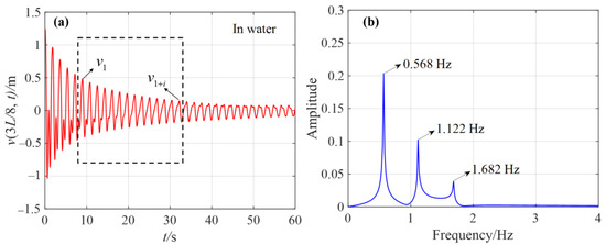
Figure 10.
Time history (a) and amplitude spectrum of displacement (b) of the anchor cable at 3L/8 in water with .
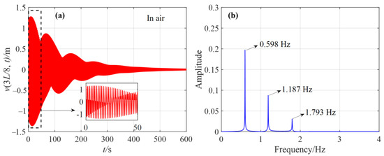
Figure 11.
Time history (a) and amplitude spectrum of displacement (b) of the cable at 3L/8 in air.
Comparing Figure 10a and Figure 11a, it can be found that the anchor cable’s vibration energy is quickly dissipated due to the hydrodynamic damping force. The time required for the amplitude to reach a steady state is much less than that in the free vibration of the tension cable in air. It indicates that the hydrodynamic damping force is beneficial to control the vibration of the STAC system. Comparing the free attenuation vibration of the anchor cable in the same period (0–50 s), we can find that the hydrodynamic damping force plays a dominant role in attenuating the free vibration of the anchor cable compared with the material damping force. In addition, according to Equation (57) and , in Figure 10a, the damping ratio of the anchor cable in water is calculated to be about 1.47%, which is much larger than the material damping ratio of the STAC.
Combined with the amplitude spectrum of displacement in Figure 10b and Figure 11b, Table 7 lists the frequency calculation results of the STAC in different media, where in the column of the improved Galerkin method, the first-order frequency and the second-order frequency are calculated by the analytical solution of the in-plane vibrational modes in Equations (19) and (12), respectively. From the comparison results in Table 7, it can be found that in the same medium, the differences between the analytical solution and the numerical solution of the frequency are minor (the relative errors are less than 1%). In different mediums, the vibration frequency of the STAC in still water is less than its vibration frequency in air (the relative errors are more significant than 5%). The reason for this can be seen in Equations (12), (19) and (33), as the movement of the STAC drives the movement of the surrounding water body, the increased additional mass decreases its frequency. In addition, according to Equation (49) given in this paper, it can be seen that the QDC will also have a certain effect on the frequency of the STAC. The degree of effect will be discussed in Section 5.4.
Table 7.
Frequency results of STAC in different mediums. (unit: Hz).
5.4. Effect of QDC on Vibration Frequency
According to the STAC’s parameters in Table 2, the initial tension is taken, and the corresponding QDCs are calculated from the drag coefficients under different working conditions. The vibration frequency of the STAC is calculated by different methods as shown in Table 8. The analytical solution of the frequency without considering is calculated by Equations (12) and (19) at this time, at which time the frequency of each order of the STAC does not change with . The analytical solution for the frequency considering is calculated by Equation (49). It can be found from Table 8 that there is a smaller error (less than 1%) between the analytical solution obtained by Equation (49) and the numerical solution of the STAC’s frequency. Overall, the relative errors between the results of the two analytical methods and the numerical results are within 2%, which is small from the point of view of the engineering tolerance (5%).
Table 8.
Comparison of STAC’s frequencies for different QDCs (unit: Hz).
5.5. Cable Tension Identification
In Section 5.4, it can be seen that the QDCs have little effect on the frequency of the STAC within the range of the effective drag force coefficients . Besides confirming the accuracy of the proposed cable tension identification (Equations (53) and (54)), this section will also investigate the sensitivity of to the results of cable tension identification. It is important to highlight that the frequency unit in Equations (51)–(54) is .
Table 9 gives a comparison of the values of the cable tension calculated by the different identification methods for different initial cable tension at the drag force coefficient (), from which it can be found the following:
Table 9.
Comparison of different cable tension identification methods with .
(1) Utilizing the first-order frequency (symmetrical): when the initial cable tension is large, such as , , as shown in Table 9, the errors in the cable tension identified by the various methods are small (all within 5%). When the initial cable tension is small, such as , , the errors of the cable tension calculated by the conventional method of Equation (51) [41] and the identification method of Equation (52) [17] are large, among which the identification error of the conventional method of Equation (51) at reaches 1217%, which is totally unacceptable. The errors of the identified cable tensions by Equation (54) given in this paper, with or without considering the effect of the QDC , are small (all less than 3%) and satisfy the engineering tolerance error.
(2) Utilizing the second-order frequency (antisymmetric): the cable tension identified by various methods in Table 9 are all within engineering tolerances (all less than 5%). The main reason can be seen from Equations (12) and (19), where when the modal order is even, the sag (or initial cable tension) has no effect on the natural frequency of the STAC. Therefore, the cable tension H can be directly calculated by Equation (53), which eliminates the iterative process of the identified cable tension such as in Equation (52) (with n as an odd number) and Equation (54). Therefore, even order frequencies can be preferred in the identified cable tension.
(3) It can be seen in Table 9 that the relative errors between initial cable tension and the identified cable tension by the improved method with are smaller than the relative errors between the identified tension of Equations (53) and (54) without and the same , and the identified cable tension without considering the effect of is conservative. Although the relative errors between the two identified tensions and are within 5%, the improved tension identification method considering the effect of is more convenient for the refined analysis of the STAC’s structure.
Based on the analysis results in Table 9, the second-order frequency of the STAC is chosen for the identified cable tension, facilitating comparison across different drag force coefficients , as shown in Table 10. Taking the initial cable tension , substituting the second-order frequency of the STAC in Table 9 into Equation (53) yields the identified cable tensions without considering . Additionally, the values of the identified cable tensions using the improved method, considering according to Equation (49), are determined. the relative error between the identified cable tension using the improved method and the initial cable tension is then calculated.
Table 10.
Comparison of identified cable tensions with different drag coefficients .
It can be seen from Table 10 that with the increase in the drag force coefficient , there is a tendency for the error of the identified cable tension H using Equation (53) without considering to increase. While in contrast the identified results of the improved method in this paper that considers have a smaller error (all are less than 0.4%), and the improved tension identification are more stable. In the range of given in this paper, although the calculated results of the conventional cable tension identification Equation (53) are acceptable within the engineering tolerance error range (5%), the difference between the conventional cable tension identification results and the initial cable tension reaches 820 kN when , which is difficult to be used for the refined analysis and state assessment of the STAC’s structure. It can be predicted that with the further increase in , its effect on the identified cable tension will gradually increase. Therefore, in practical engineering, it is recommended to adopt the improved tension identification method given in this paper, considering the effect of drag force coefficients , which can improve the accuracy of identifying the cable tension of STACs to a certain extent.
6. Conclusions
In this paper, the consideration of bending stiffness is within the static equilibrium equation of the STAC, where the bending stiffness influence coefficient and Irvine parameter are introduced to derive the analytical model of in-plane modal frequency and modal shape. On this basis, an improved Galerkin method is proposed to discretize the nonlinear free motion equation of the STAC. Subsequently, the analytical solution for the nonlinear free vibration response of the STAC is derived, incorporating improvements such as the averaging method, frequency formulas, and tension identification method that account for QDC. Finally, the theory presented in this paper is validated and analyzed using a typical floating structure mooring cable. Based on the results and discussions, the following conclusions can be drawn:
(1) The antisymmetric modal frequency of the STAC is independent of , while the modal shapes are only related to the modal order, and has nothing to do with and . With the increase of the modal order n, the effect of on the antisymmetric modal frequency gradually increases. When , the effect of bending stiffness on the first two modal frequencies can be ignored.
(2) and can control the symmetrical vibration of the STAC similar to the motion of the cable, beam, and cable–beam: when (or ), the STAC is similar to the Euler beam, and the effect of on its natural frequency can be ignored. When (or ), the STAC is equivalent to changing from a taut string model to a cable model as increases. When , the modal characteristics can be considered to be between the cable and the beam.
(3) The exact frequency given in this paper is basically consistent with the FEM results, while the results obtained by the conventional Galerkin method have a large error with the FEM results when the initial tension is small. The displacement responses at this time are quite different from the results of the improved Galerkin method, which indicates that the traditional Galerkin method has certain limitations in the analysis of the vibration characteristics of the STAC.
(4) The hydrodynamic damping force plays a dominant role in the attenuation of the free vibration of the STAC compared to the cable’s dynamic responses in air. The effect of the additional mass makes the cable’s frequency in still water smaller than its frequency in air. Furthermore, the improved frequency (Equation (49)) based on the improved average method can quantitatively describe the effect of QDC, and the error between the numerical solution and Equation (49) is within 1%.
(5) The effect of the STAC’s sag on the even order frequency can be neglected, so the identified cable tension can give priority to the even order frequency, which can save the iterative process of cable tension identification. In addition, in practical engineering, in order to obtain more accurate identified cable tension, it is recommended to adopt the improved tension identification method given in this paper considering QDC.
Author Contributions
Conceptualization, L.Y.; methodology, L.Y. and D.W.; investigation, H.Z., Z.M. and Y.Z.; writing-original draft, L.Y.; writing-review and editing, L.Y. and H.Z.; software, L.Y. and Y.Z.; validation, L.Y.; visualization, L.Y.; formal analysis, D.W., H.Z. and Z.M.; funding acquisition, H.Z. and D.W.; supervision, D.W. All authors have read and agreed to the published version of the manuscript.
Funding
Support from the National Natural Science Foundation of China (NSFC), under grant number 51878527 and 52308199, is greatly acknowledged. The authors would also like to appreciate the Natural Science Foundation of Hainan Province, China (No. 523QN265).
Institutional Review Board Statement
Not applicable.
Informed Consent Statement
Not applicable.
Data Availability Statement
The original contributions presented in the study are included in the article, further inquiries can be directed to the corresponding authors.
Conflicts of Interest
The authors declare no conflicts of interest.
References
- Han, F.; Deng, Z.; Dan, D. Modelling and analysis framework for nonlinear dynamics of submerged tensioned cables. Ocean Eng. 2021, 232, 109123. [Google Scholar] [CrossRef]
- Han, F.; Han, L.; Deng, Z.; Chen, L. An analytical method for nonlinear vibration analysis of submerged tensioned anchors. Nonlinear Dyn. 2023, 111, 11001–11022. [Google Scholar]
- Tabeshpour, M.R.; Abbasian, S.M.R.S. The optimum mooring configuration with minimum sensitivity to remove a mooring line for a semi-submersible platform. Appl. Ocean Res. 2021, 114, 102766. [Google Scholar] [CrossRef]
- Zhu, X.; Wang, Y.; Yoo, W.S.; Nicoll, R.; Ren, H. Stability analysis of spar platform with four mooring cables in consideration of cable dynamics. Ocean Eng. 2021, 236, 109522. [Google Scholar] [CrossRef]
- Xu, X.; Wei, N.; Yao, W. The stability analysis of Tension-Leg Platforms under marine environmental loads via altering the connection angle of tension legs. Water 2022, 14, 283. [Google Scholar] [CrossRef]
- Thiagarajan, K.P.; Dagher, H.J. A review of floating platform concepts for offshore wind energy generation. J. Offshore Mech. Arct. Eng. 2014, 136, 020903. [Google Scholar] [CrossRef]
- Zhao, Z.; Wang, W.; Shi, W.; Li, X. Effects of second-order hydrodynamics on an ultra-large semi-submersible floating offshore wind turbine. Structure 2020, 28, 2260–2275. [Google Scholar] [CrossRef]
- Zhang, L.; Michailides, C.; Wang, Y.; Shi, W. Moderate water depth effects on the response of a floating wind turbine. Structure 2020, 28, 1435–1448. [Google Scholar] [CrossRef]
- Han, Y.; Le, C.; Ding, H.; Cheng, Z.; Zhang, P. Stability and dynamic response analysis of a submerged tension leg platform for offshore wind turbines. Ocean Eng. 2017, 129, 68–82. [Google Scholar] [CrossRef]
- Xu, Y.; Øiseth, O.; Moan, T. Time domain simulations of wind-and wave-induced load effects on a three-span suspension bridge with two floating pylons. Mar. Struct. 2018, 58, 434–452. [Google Scholar] [CrossRef]
- Wang, J.; Cheynet, E.; Snæbjörnsson, J.P.; Jakobsen, J.B. Coupled aerodynamic and hydrodynamic response of a long span bridge suspended from floating towers. J. Wind Eng. Ind. Aerod. 2018, 177, 19–31. [Google Scholar] [CrossRef]
- Zhang, H.; Yang, Z.; Li, J.; Yuan, C.; Xie, M.; Yang, H.; Yin, H. A global review for the hydrodynamic response investigation method of submerged floating tunnels. Ocean Eng. 2021, 225, 108825. [Google Scholar] [CrossRef]
- Lu, W.; Ge, F.; Wang, L.; Wu, X.; Hong, Y. On the slack phenomena and snap force in tethers of submerged floating tunnels under wave conditions. Mar. Struct. 2011, 24, 358–376. [Google Scholar] [CrossRef]
- Wu, Z.; Ni, P.; Mei, G. Vibration response of cable for submerged floating tunnel under simultaneous hydrodynamic force and earthquake excitations. Adv. Struct. Eng. 2018, 21, 1761–1773. [Google Scholar] [CrossRef]
- Sun, S.; Su, Z.; Feng, Y. Nonlinear vibration analysis of submerged floating tunnel tether. Adv. Civ. Eng. 2020, 2020, 8885712. [Google Scholar] [CrossRef]
- Won, D.; Park, W.S.; Kang, Y.J.; Kim, S. Dynamic behavior of the submerged floating tunnel moored by inclined tethers attached to fixed towers. Ocean Eng. 2021, 237, 109663. [Google Scholar] [CrossRef]
- Han, F.; Duan, Z.Y. Research on dynamic response analysis and cable force identification method of submerged anchor cables. Chin. J. Theor. Appl. Mech. 2022, 54, 921–928. [Google Scholar]
- Chen, Z.; Xiang, Y.; Lin, H.; Yang, Y. Coupled vibration analysis of submerged floating tunnel system in wave and current. Appl. Sci. 2018, 8, 1311. [Google Scholar] [CrossRef]
- Hall, M.; Goupee, A. Validation of a lumped-mass mooring line model with DeepCwind semisubmersible model test data. Ocean Eng. 2015, 104, 590–603. [Google Scholar] [CrossRef]
- Touzon, I.; Nava, V.; Gao, Z.; Petuya, V. Frequency domain modelling of a coupled system of floating structure and mooring lines: An application to a wave energy converter. Ocean Eng. 2021, 220, 108498. [Google Scholar] [CrossRef]
- Lee, H.W.; Roh, M.I. Review of the multibody dynamics in the applications of ships and offshore structures. Ocean Eng. 2018, 167, 65–76. [Google Scholar] [CrossRef]
- Yang, C.; Liu, Y.; Du, J.; Cheng, Z.; Wang, H. Nonlinear dynamic optimization of marine riser system anti-recoil under a flexible multibody framework. Ocean Eng. 2023, 281, 114666. [Google Scholar] [CrossRef]
- Xiang, Y.Q.; Chao, C.F. Vortex-induced dynamic response analysis for the submerged floating tunnel system under the effect of currents. J. Waterw. Port. Coast. Ocean Eng. 2013, 139, 183–189. [Google Scholar]
- Han, F.; Zhang, Y.; Zang, J.; Zhen, N. Exact dynamic analysis of shallow sagged cable system—Theory and experimental verification. Int. J. Struct. Stab. Dyn. 2019, 19, 1950153. [Google Scholar] [CrossRef]
- Wang, K.; Er, G.K.; Zhu, Z. 3D nonlinear dynamic analysis of cable-moored offshore structures. Ocean Eng. 2020, 213, 107759. [Google Scholar] [CrossRef]
- Zhang, Y.; Shi, W.; Li, D.; Li, X.; Duan, Y. Development of a numerical mooring line model for a floating wind turbine based on the vector form intrinsic finite element method. Ocean Eng. 2022, 253, 111354. [Google Scholar] [CrossRef]
- Irvine, H.M. Cable Structures; MIT Press: Cambridge, MA, USA, 1981. [Google Scholar]
- Ricciardi, G.; Saitta, F. A continuous vibration analysis model for cables with sag and bending stiffness. Eng. Struct. 2008, 30, 1459–1472. [Google Scholar] [CrossRef]
- Ni, Y.Q.; Ko, J.M.; Zheng, G. Dynamic analysis of large-diameter sagged cables taking into account flexural rigidity. J. Sound Vib. 2002, 257, 301–319. [Google Scholar] [CrossRef]
- Kang, H.J.; Zhao, Y.Y.; Zhu, H.P. Linear and nonlinear dynamics of suspended cable considering bending stiffness. J. Vib. Control 2015, 21, 1487–1505. [Google Scholar] [CrossRef]
- Han, F.; Dan, D. Free vibration of the complex cable system—An exact method using symbolic computation. Mech. Syst. Signal Process. 2020, 139, 106636. [Google Scholar]
- Cantero, D.; Rønnquist, A.; Naess, A. Tension during parametric excitation in submerged vertical taut tethers. Appl. Ocean Res. 2017, 65, 279–289. [Google Scholar] [CrossRef]
- Papazoglou, V.J.; Mavrakos, S.A.; Triantafyllou, M.S. Non-linear cable response and model testing in water. J. Sound Vib. 1990, 140, 103–115. [Google Scholar] [CrossRef]
- Ibrahim, R.A. Nonlinear vibrations of suspended cables, Part III: Random excitation and interaction with fluid flow. Appl. Mech. Rev. 2004, 57, 515–549. [Google Scholar] [CrossRef]
- Hayashi, C. Nonlinear Oscillations in Physical Systems; Princeton University Press: Princeton, NJ, USA, 1986. [Google Scholar]
- Hou, Z.; Yuan, K.; Xie, F.; Jin, H.; Shi, Q. Oscillation properties of a simple pendulum in a viscous liquid. Eur. J. Phys. 2014, 36, 015011. [Google Scholar] [CrossRef]
- Zhang, W.; Gao, Y.H.; Lu, S.F. Theoretical, numerical and experimental researches on time-varying dynamics of telescopic wing. J. Sound Vib. 2022, 522, 116724. [Google Scholar] [CrossRef]
- Du, J.; Wang, H.; Wang, S.; Song, X.; Wang, J.; Chang, A. Fatigue damage assessment of mooring lines under the effect of wave climate change and marine corrosion. Ocean Eng. 2020, 206, 107303. [Google Scholar] [CrossRef]
- Dai, J.; Leira, B.J.; Moan, T.; Alsos, H.S. Effect of wave inhomogeneity on fatigue damage of mooring lines of a side-anchored floating bridge. Ocean Eng. 2021, 219, 108304. [Google Scholar] [CrossRef]
- Ibarra, M.A.C.; Simão, M.L.; Videiro, P.M.; Sagrilo, L.V.S. Long-term fatigue analysis of mooring lines considering wind-sea and swell waves using the Univariate Dimension-Reduction Method. Appl. Ocean Res. 2022, 118, 102997. [Google Scholar] [CrossRef]
- Zui, H.; Shinke, T.; Namita, Y. Practical formulas for estimation of cable tension by vibration method. J. Struct. Eng. 1996, 122, 651–656. [Google Scholar] [CrossRef]
- Ma, L. A highly precise frequency-based method for estimating the tension of an inclined cable with unknown boundary conditions. J. Sound Vib. 2017, 409, 65–80. [Google Scholar] [CrossRef]
- Mehrabi, A.B.; Tabatabai, H. Unified finite difference formulation for free vibration of cables. J. Struct. Eng. 1998, 124, 1313–1322. [Google Scholar] [CrossRef]
- Ren, W.X.; Chen, G.; Hu, W.H. Empirical formulas to estimate cable tension by cable fundamental frequency. Struct. Eng. Mech. 2005, 20, 363–380. [Google Scholar] [CrossRef]
- He, W.Y.; Meng, F.C.; Ren, W.X. Cable force estimation of cables with small sag considering inclination angle effect. Adv. Bridge Eng. 2021, 2, 15. [Google Scholar] [CrossRef]
- Treyssede, F. Free linear vibrations of cables under thermal stress. J. Sound Vib. 2009, 327, 1–8. [Google Scholar] [CrossRef][Green Version]
- Clough, R.W.; Penzien, J. Dynamic of Structures; McGraw-Hill: New York, NY, USA, 1975. [Google Scholar]
- Zhang, X.; Xu, H.; Cao, M.; Sumarac, D.; Lu, Y.; Peng, J. In-plane free vibrations of small-sag inclined cables considering bending stiffness with applications to cable tension identification. J. Sound Vib. 2023, 544, 117394. [Google Scholar] [CrossRef]
- Morison, J.R.; Johnson, J.W.; Schaaf, S.F. The force exerted by surface waves on piles. J. Petrol. Technol. 1950, 2, 149–154. [Google Scholar] [CrossRef]
- Recommended Practice DNV-RP-C205, Environmental Conditions and Environmental Loads; Det Norske Veritas: Bærum, Norway, 2010.
- Irvine, H.M.; Caughey, T.K. The linear theory of free vibrations of a suspended cable. Proc. R. Soc. Lond. A Math. Phys. Sci. 1974, 341, 299–315. [Google Scholar]
- Wang, Z.Q.; Wang, L.H.; Liu, Q.J.; Zhao, Y.B. Solutions of a dynamics nonlinear in-plane vibration of suspended cable investigated by the mixed averaging method. Appl. Mech. Mater. 2013, 275, 869–882. [Google Scholar] [CrossRef]
- Wang, D.H.; Chen, X.Z.; Xu, K. Analysis of buffeting response of hinged overhead transmission conductor to nonstationary winds. Eng. Struct. 2017, 147, 567–582. [Google Scholar] [CrossRef]
- Zhao, Y.; Sun, C.; Wang, Z.; Wang, L. Approximate series solutions for nonlinear free vibration of suspended cables. Shock Vib. 2014, 2014, 795708. [Google Scholar] [CrossRef]


Disclaimer/Publisher’s Note: The statements, opinions and data contained in all publications are solely those of the individual author(s) and contributor(s) and not of MDPI and/or the editor(s). MDPI and/or the editor(s) disclaim responsibility for any injury to people or property resulting from any ideas, methods, instructions or products referred to in the content. |
© 2024 by the authors. Licensee MDPI, Basel, Switzerland. This article is an open access article distributed under the terms and conditions of the Creative Commons Attribution (CC BY) license (https://creativecommons.org/licenses/by/4.0/).