
A New Cross-Domain Motor Fault Diagnosis Method Based on Bimodal Inputs


Abstract
1. Introduction
2. Basic Theory
2.1. Continuous Wavelet Transform
2.2. Park Transformation
2.3. ResNet Network Model Structure
2.4. Swin Transformer Model Structure
3. Intelligent Diagnostic Model for Multi-Modal Cross-Domain Motor
4. Collection of Experimental Data and Construction of Fault Samples
4.1. Setup of Experimental Platform
4.2. Construction of Experimental Dataset
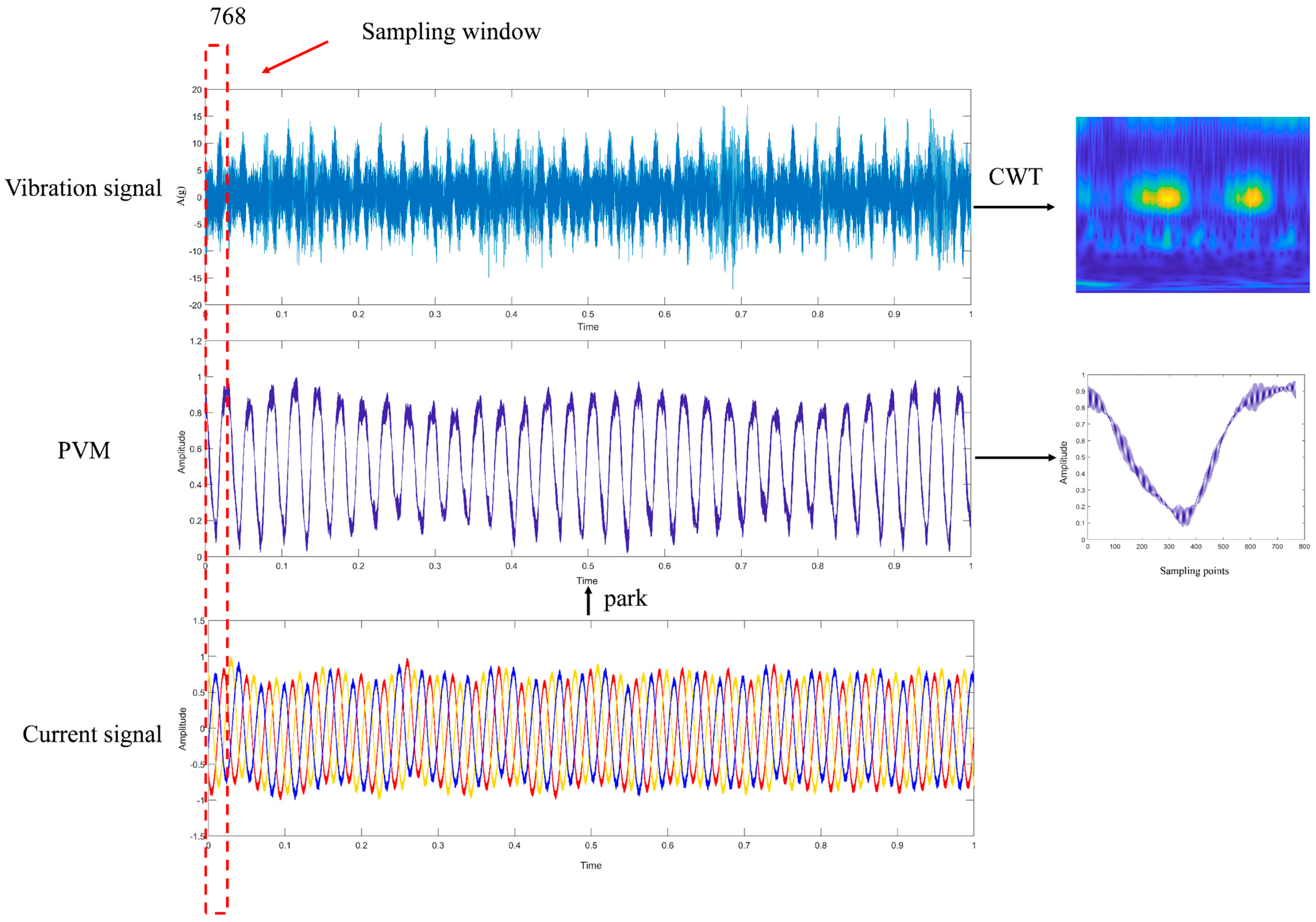
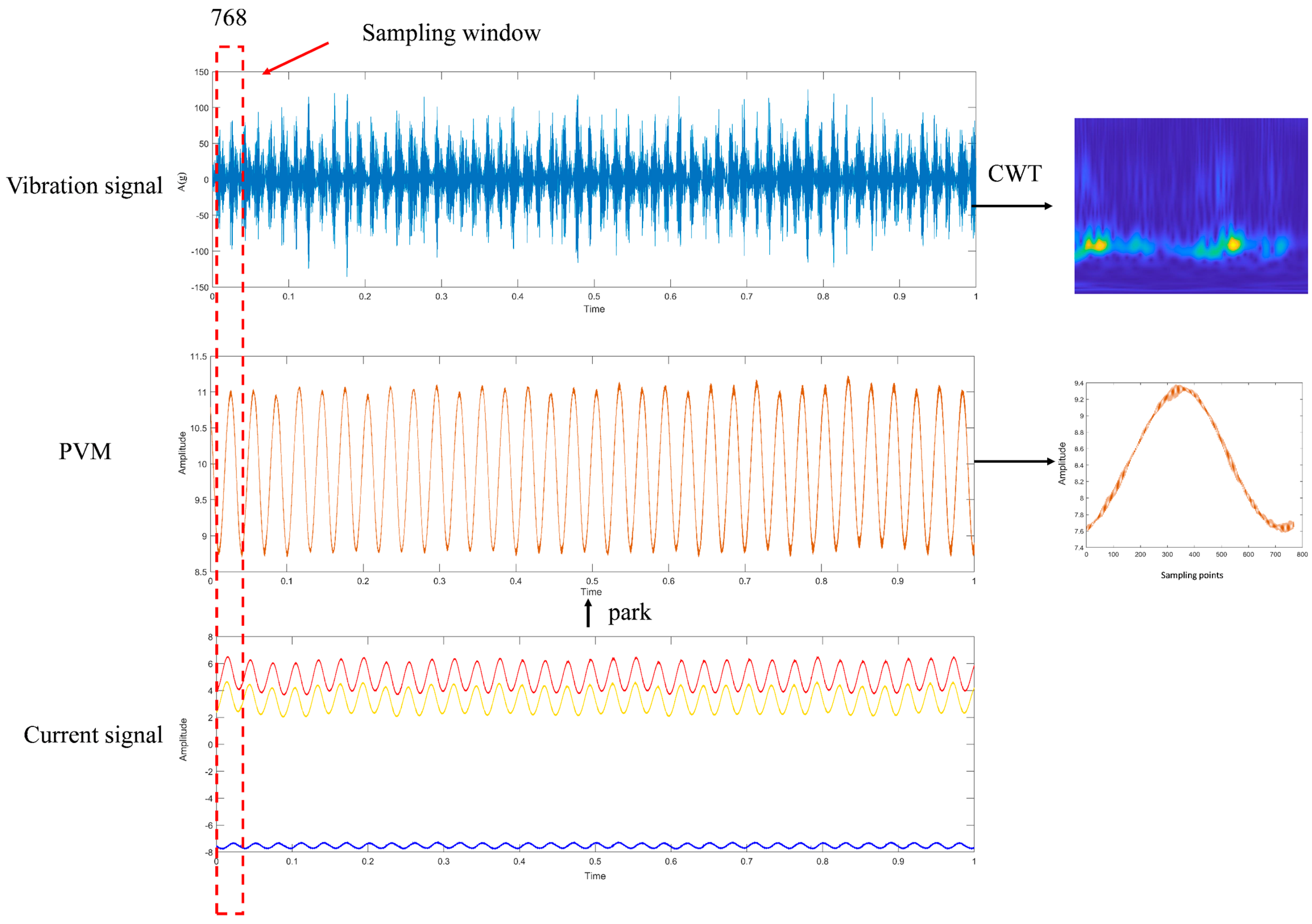
4.2.1. Fault Sample Feature Extraction
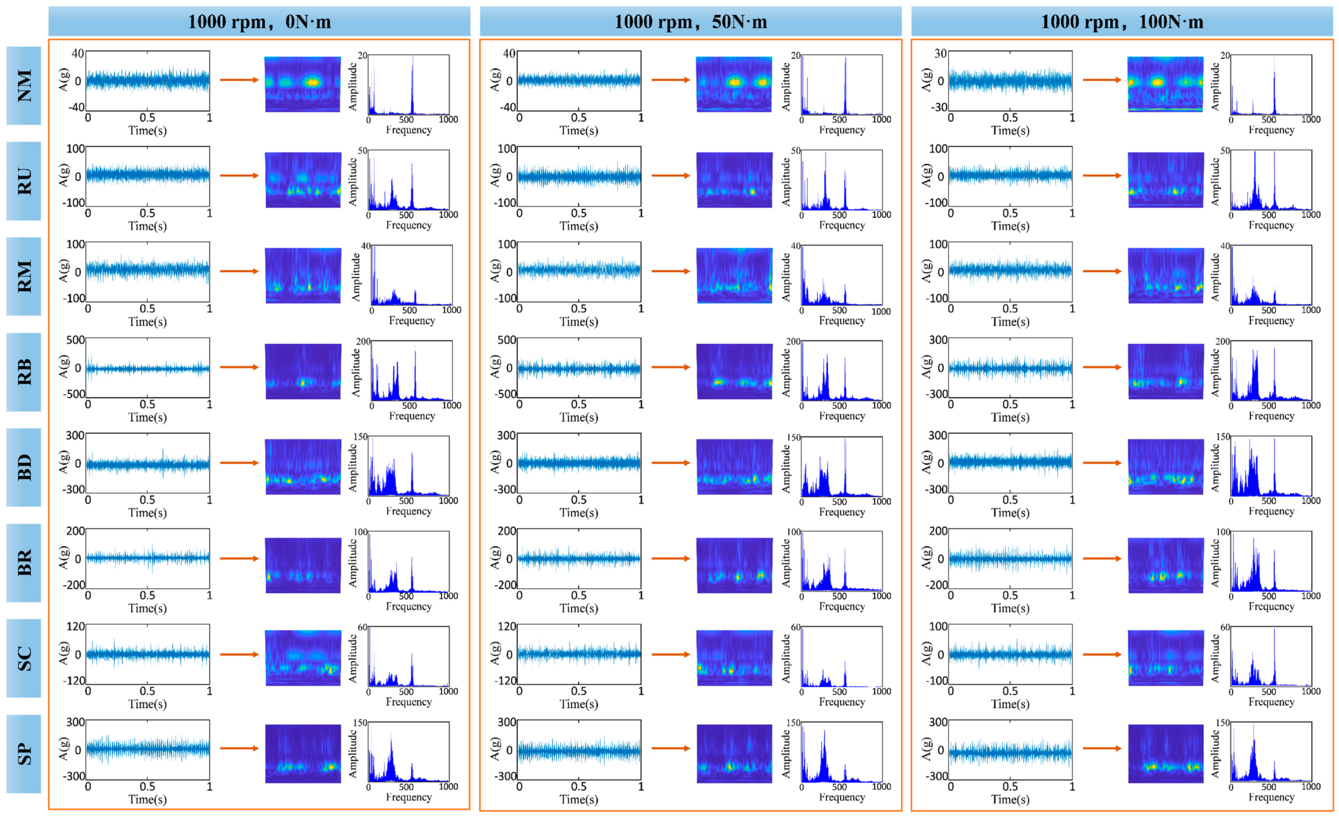
4.2.2. Fault Sample Data Analysis
4.2.3. Constructing Fault Sample Library
5. Results and Discussion
5.1. Comparison Experiment Analysis of Single-Modal Models
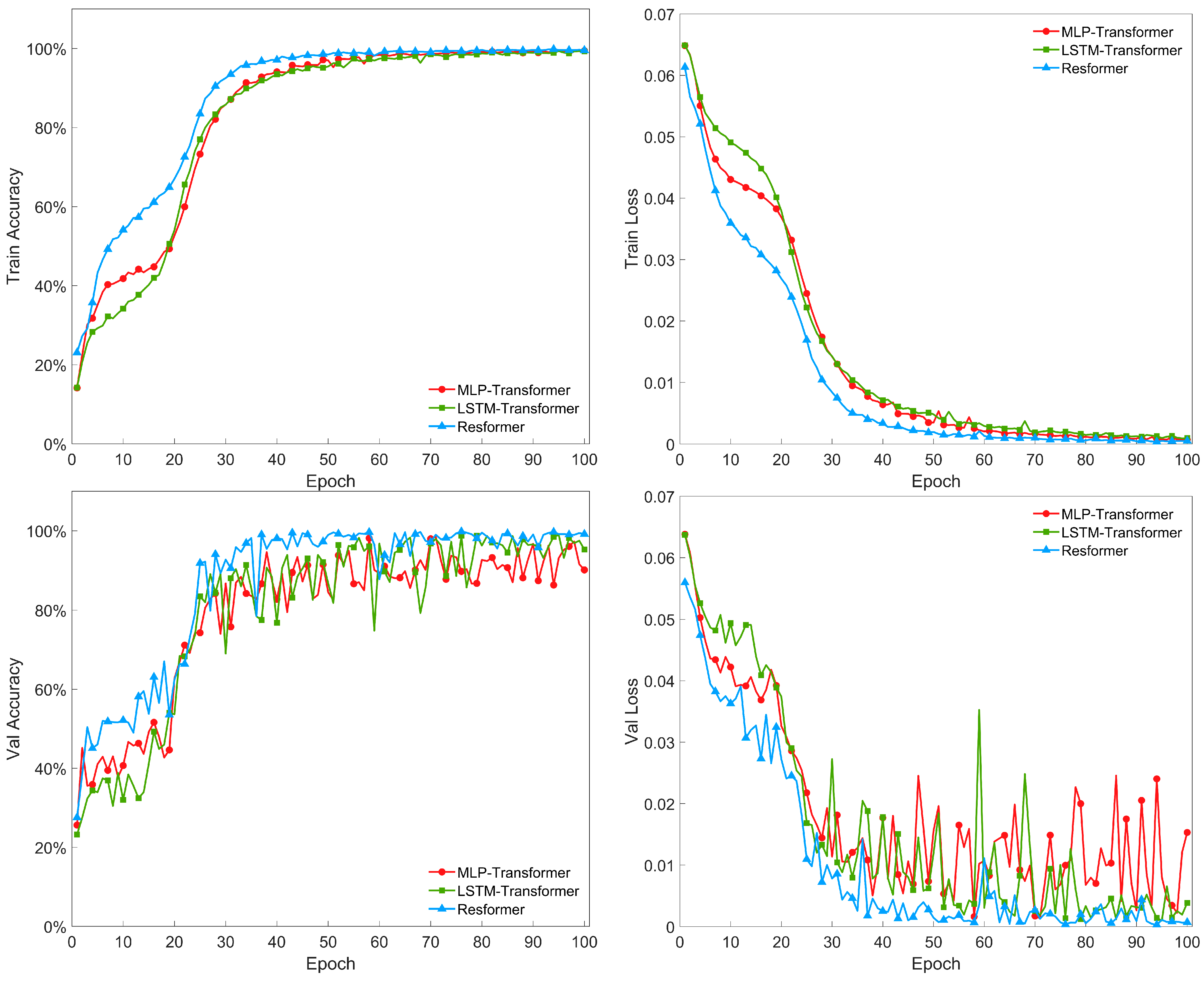
5.2. Comparison Experiment Analysis of Double-Modal Models
5.3. Performance Analysis of the Resformer Model
6. Conclusions
Author Contributions
Funding
Institutional Review Board Statement
Informed Consent Statement
Data Availability Statement
Conflicts of Interest
References
- Huang, G.; Tang, Y.; Chen, X.; Chen, M.; Jiang, Y. A Comprehensive Review of Floating Solar Plants and Potentials for Offshore Applications. J. Mar. Sci. Eng. 2023, 11, 2064. [Google Scholar] [CrossRef]
- Chen, M.; Jiang, J.; Zhang, W.; Li, C.B.; Zhou, H.; Jiang, Y.; Sun, X. Study on Mooring Design of 15 MW Floating Wind Turbines in South China Sea. J. Mar. Sci. Eng. 2024, 12, 33. [Google Scholar] [CrossRef]
- Zhang, Z.; Kuang, L.; Zhao, Y.; Han, Z.; Zhou, D.; Tu, J.; Chen, M.; Ji, X. Numerical investigation of the aerodynamic and wake characteristics of a floating twin-rotor wind turbine under surge motion. Energy Convers. Manag. 2023, 283, 116957. [Google Scholar] [CrossRef]
- Chen, M.; Deng, J.; Yang, Y.; Zhou, H.; Tao, T.; Liu, S.; Sun, L.; Hua, L. Performance Analysis of a Floating Wind–Wave Power Generation Platform Based on the Frequency Domain Model. J. Mar. Sci. Eng. 2024, 12, 206. [Google Scholar] [CrossRef]
- Inal, O.B.; Charpentier, J.-F.; Deniz, C. Hybrid power and propulsion systems for ships: Current status and future challenges. Renew. Sustain. Energy Rev. 2022, 156, 111965. [Google Scholar] [CrossRef]
- Chen, M.; Chen, Y.; Li, T.; Tang, Y.; Ye, J.; Zhou, H.; Ouyang, M.; Zhang, X.; Shi, W.; Sun, X. Analysis of the wet-towing operation of a semi-submersible floating wind turbine using a single tugboat. Ocean Eng. 2024, 299. [Google Scholar] [CrossRef]
- Nuchturee, C.; Li, T.; Xia, H. Energy efficiency of integrated electric propulsion for ships—A review. Renew. Sustain. Energy Rev. 2020, 134, 110145. [Google Scholar] [CrossRef]
- Serra, P.; Fancello, G. Towards the IMO’s GHG Goals: A Critical Overview of the Perspectives and Challenges of the Main Options for Decarbonizing International Shipping. Sustainability 2020, 12, 3220. [Google Scholar] [CrossRef]
- Geertsma, R.D.; Negenborn, R.R.; Visser, K.; Hopman, J.J. Design and control of hybrid power and propulsion systems for smart ships: A review of developments. Appl. Energy 2017, 194, 30–54. [Google Scholar] [CrossRef]
- Choudhary, A.; Goyal, D.; Letha, S.S. Infrared Thermography-Based Fault Diagnosis of Induction Motor Bearings Using Machine Learning. IEEE Sens. J. 2021, 21, 1727–1734. [Google Scholar] [CrossRef]
- Xu, X.; Yan, X.; Yang, K.; Zhao, J.; Sheng, C.; Yuan, C. Review of condition monitoring and fault diagnosis for marine power systems. Transp. Saf. Environ. 2021, 3, 85–102. [Google Scholar] [CrossRef]
- Chegini, S.N.; Bagheri, A.; Najafi, F. Application of a new EWT-based denoising technique in bearing fault diagnosis. Measurement 2019, 144, 275–297. [Google Scholar] [CrossRef]
- Abdelkader, R.; Kaddour, A.; Bendiabdellah, A.; Derouiche, Z. Rolling Bearing Fault Diagnosis Based on an Improved Denoising Method Using the Complete Ensemble Empirical Mode Decomposition and the Optimized Thresholding Operation. IEEE Sens. J. 2018, 18, 7166–7172. [Google Scholar] [CrossRef]
- Wang, T.; Chu, F. Bearing fault diagnosis under time-varying rotational speed via the fault characteristic order (FCO) index based demodulation and the stepwise resampling in the fault phase angle (FPA) domain. ISA Trans. 2019, 94, 391–400. [Google Scholar] [CrossRef] [PubMed]
- Choudhary, A.; Mishra, R.K.; Fatima, S.; Panigrahi, B.K. Multi-input CNN based vibro-acoustic fusion for accurate fault diagnosis of induction motor. Eng. Appl. Artif. Intell. 2023, 120, 105872. [Google Scholar] [CrossRef]
- Ren, B.; Yang, M.; Chai, N.; Li, Y.; Xu, D. Fault Diagnosis of Motor Bearing Based on Speed Signal Kurtosis Spectrum Analysis. In Proceedings of the 2019 22nd International Conference on Electrical Machines and Systems (ICEMS), Harbin, China, 11–14 August 2019; pp. 1–6. [Google Scholar]
- AlShorman, O.; Alkahatni, F.; Masadeh, M.; Irfan, M.; Glowacz, A.; Althobiani, F.; Kozik, J.; Glowacz, W. Sounds and acoustic emission-based early fault diagnosis of induction motor: A review study. Adv. Mech. Eng. 2021, 13, 1687814021996915. [Google Scholar] [CrossRef]
- Zhou, Y.; Shang, Q.; Guan, C. Three-Phase Asynchronous Motor Fault Diagnosis Using Attention Mechanism and Hybrid CNN-MLP by Multi-Sensor Information. IEEE Access 2023, 11, 98402–98414. [Google Scholar] [CrossRef]
- Xie, F.; Li, G.; Hu, W.; Fan, Q.; Zhou, S. Intelligent Fault Diagnosis of Variable-Condition Motors Using a Dual-Mode Fusion Attention Residual. J. Mar. Sci. Eng. 2023, 11, 1385. [Google Scholar] [CrossRef]
- Bessam, B.; Menacer, A.; Boumehraz, M.; Cherif, H. Detection of broken rotor bar faults in induction motor at low load using neural network. ISA Trans. 2016, 64, 241–246. [Google Scholar] [CrossRef]
- Zhao, R.; Yan, R.; Chen, Z.; Mao, K.; Wang, P.; Gao, R.X. Deep learning and its applications to machine health monitoring. Mech. Syst. Signal Process. 2019, 115, 213–237. [Google Scholar] [CrossRef]
- Hinton, G.E.; Osindero, S.; Teh, Y.W. A fast learning algorithm for deep belief nets. Neural Comput. 2006, 18, 1527–1554. [Google Scholar] [CrossRef] [PubMed]
- Wang, F.; Liu, R.; Hu, Q.; Chen, X. Cascade Convolutional Neural Network with Progressive Optimization for Motor Fault Diagnosis under Nonstationary Conditions. IEEE Trans. Ind. Inform. 2021, 17, 2511–2521. [Google Scholar] [CrossRef]
- Xin, G.; Li, Z.; Jia, L.; Zhong, Q.; Dong, H.; Hamzaoui, N.; Antoni, J. Fault Diagnosis of Wheelset Bearings in High-Speed Trains Using Logarithmic Short-Time Fourier Transform and Modified Self-Calibrated Residual Network. IEEE Trans. Ind. Inform. 2022, 18, 7285–7295. [Google Scholar] [CrossRef]
- Jia, N.; Cheng, Y.; Liu, Y.; Tian, Y. Intelligent Fault Diagnosis of Rotating Machines Based on Wavelet Time-Frequency Diagram and Optimized Stacked Denoising Auto-Encoder. IEEE Sens. J. 2022, 22, 17139–17150. [Google Scholar] [CrossRef]
- Tang, H.; Liao, Z.; Chen, P.; Zuo, D.; Yi, S. A Novel Convolutional Neural Network for Low-Speed Structural Fault Diagnosis Under Different Operating Condition and Its Understanding via Visualization. IEEE Trans. Instrum. Meas. 2021, 70, 1–11. [Google Scholar] [CrossRef]
- Sun, Y.; Li, S.; Wang, X.J.M. Bearing fault diagnosis based on EMD and improved Chebyshev distance in SDP image. Measurement 2021, 176, 109100. [Google Scholar] [CrossRef]
- Xie, J.-L.; Shi, W.-F.; Xue, T.; Liu, Y.-H. High-Resistance Connection Fault Diagnosis in Ship Electric Propulsion System Using Res-CBDNN. J. Mar. Sci. Eng. 2024, 12, 583. [Google Scholar] [CrossRef]
- Zhu, Y.; Su, H.; Tang, S.; Zhang, S.; Zhou, T.; Wang, J. A Novel Fault Diagnosis Method Based on SWT and VGG-LSTM Model for Hydraulic Axial Piston Pump. J. Mar. Sci. Eng. 2023, 11, 594. [Google Scholar] [CrossRef]
- Vaswani, A.; Shazeer, N.; Parmar, N.; Uszkoreit, J.; Jones, L.; Gomez, A.N.; Kaiser, Ł.; Polosukhin, I. Attention is all you need. arXiv 2017, arXiv:1706.03762. [Google Scholar]
- Jin, Y.; Hou, L.; Chen, Y. A new rotating machinery fault diagnosis method based on the Time Series Transformer. arXiv 2021, arXiv:2108.12562. [Google Scholar]
- Wu, H.; Triebe, M.J.; Sutherland, J.W. A transformer-based approach for novel fault detection and fault classification/diagnosis in manufacturing: A rotary system application. J. Manuf. Syst. 2023, 67, 439–452. [Google Scholar] [CrossRef]
- Ding, Y.; Jia, M.; Miao, Q.; Cao, Y. A novel time–frequency Transformer based on self–attention mechanism and its application in fault diagnosis of rolling bearings. Mech. Syst. Signal Process. 2022, 168, 108616. [Google Scholar] [CrossRef]
- Yan, R.; Gao, R.X.; Chen, X. Wavelets for fault diagnosis of rotary machines: A review with applications. Signal Process. 2014, 96, 1–15. [Google Scholar] [CrossRef]
- Das, S.; Purkait, P.; Dey, D.; Chakravorti, S. Monitoring of inter-turn insulation failure in induction motor using advanced signal and data processing tools. IEEE Trans. Dielectr. Electr. Insul. 2011, 18, 1599–1608. [Google Scholar] [CrossRef]
- Sonje, D.M.; Kundu, P.; Chowdhury, A. A Novel Approach for Sensitive Inter-turn Fault Detection in Induction Motor under Various Operating Conditions. Arab. J. Sci. Eng. 2019, 44, 6887–6900. [Google Scholar] [CrossRef]
- Lilly, J.M.; Olhede, S.C. Higher-Order Properties of Analytic Wavelets. IEEE Trans. Signal Process. 2009, 57, 146–160. [Google Scholar] [CrossRef]
- Douglas, H.; Pillay, P.; Barendse, P. The detection of interturn stator faults in doubly-fed induction generators. In Proceedings of the Fourtieth IAS Annual Meeting. Conference Record of the 2005 Industry Applications Conference, Hong Kong, China, 2–6 October 2005; pp. 1097–1102. [Google Scholar]
- Sonje, D.M.; Chowdhury, A.; Kundu, P. Fault diagnosis of induction motor using parks vector approach. In Proceedings of the 2014 International Conference on Advances in Electrical Engineering (ICAEE), Vellore, India, 9–11 January 2014; pp. 1–4. [Google Scholar]
- He, K.; Zhang, X.; Ren, S.; Sun, J. Deep Residual Learning for Image Recognition. In Proceedings of the 2016 IEEE Conference on Computer Vision and Pattern Recognition (CVPR), Las Vegas, NV, USA, 27–30 June 2016; pp. 770–778. [Google Scholar]
- Dosovitskiy, A.; Beyer, L.; Kolesnikov, A.; Weissenborn, D.; Zhai, X.; Unterthiner, T.; Dehghani, M.; Minderer, M.; Heigold, G.; Gelly, S.; et al. An image is worth 16 × 16 words: Transformers for image recognition at scale. arXiv 2020, arXiv:2010.11929. [Google Scholar]
- Liu, Z.; Lin, Y.; Cao, Y.; Hu, H.; Wei, Y.; Zhang, Z.; Lin, S.; Guo, B. Swin transformer: Hierarchical vision transformer using shifted windows. In Proceedings of the IEEE/CVF International Conference on Computer Vision, Montreal, QC, Canada, 10–17 October 2021; pp. 10012–10022. [Google Scholar]
- Hendrycks, D.; Gimpel, K. Gaussian error linear units (gelus). arXiv 2016, arXiv:1606.08415. [Google Scholar]
- Cano, A.; Arévalo, P.; Benavides, D.; Jurado, F. Integrating discrete wavelet transform with neural networks and machine learning for fault detection in microgrids. Int. J. Electr. Power Energy Syst. 2024, 155, 109616. [Google Scholar] [CrossRef]
- Han, H.; Wang, H.; Liu, Z.; Wang, J. Intelligent vibration signal denoising method based on non-local fully convolutional neural network for rolling bearings. ISA Trans. 2022, 122, 13–23. [Google Scholar] [CrossRef]
- Li, Y.; Cheng, G.; Liu, C. Research on bearing fault diagnosis based on spectrum characteristics under strong noise interference. Measurement 2021, 169, 108509. [Google Scholar] [CrossRef]
- Zhao, D.; Cui, L.; Liu, D. Bearing Weak Fault Feature Extraction Under Time-Varying Speed Conditions Based on Frequency Matching Demodulation Transform. IEEE/ASME Trans. Mechatron. 2023, 28, 1627–1637. [Google Scholar] [CrossRef]
- Zhao, D.; Cai, W.; Cui, L. Adaptive thresholding and coordinate attention-based tree-inspired network for aero-engine bearing health monitoring under strong noise. Adv. Eng. Inform. 2024, 61, 102559. [Google Scholar] [CrossRef]
- Simonyan, K.; Zisserman, A. Very deep convolutional networks for large-scale image recognition. arXiv 2014, arXiv:1409.1556. [Google Scholar]
- Jia, L.; Chow, T.W.S.; Yuan, Y. GTFE-Net: A Gramian Time Frequency Enhancement CNN for bearing fault diagnosis. Eng. Appl. Artif. Intell. 2023, 119, 105794. [Google Scholar] [CrossRef]


| Network Layer | Swin-t Branch | Resnet-18 Branch | ||
|---|---|---|---|---|
| Output Dimension | Layer Configuration | Output Dimension | Layer Configuration | |
| Input | 224 × 224 × 3 | - | 768 × 1 | - |
| Stage 1 | 56 × 56 × 96 | Patch Partition [4 × 4] stride 4 | 384 × 64 | Conv1d 7 × 7, stride 2 |
| 56 × 56 × 96 | Linear Embedding | 192 × 64 | Max-Pool 3 × 3, stride 2 | |
| Stage 2 | 56 × 56 × 96 | Transformer block × 2 | 192 × 64 | Residual block [3 × 3, 64] × 2 |
| Stage 3 | 28 × 28 × 192 | Patch Merging and Transformer block × 2 | 96 × 128 | Residual block [3 × 3, 128] × 2, stride 2 |
| Stage 4 | 14 × 14 × 384 | Patch Merging and Transformer block × 2 | 48× 256 | Residual block [3 × 3, 256] × 2, stride 2 |
| Stage 5 | 7 × 7 × 768 | Patch Merging and Transformer block × 2 | 24 × 512 | Residual block [3 × 3, 512] × 2, stride 2 |
| Average Pooling | 768 | Global Average Pooling | 512 | Adaptive AvgPool1d |
| Concatenation | 1280 | Concatenation of the outputs of Swin-t and ResNet-18 | ||
| MLP Layer 1 | 512 | Linear(1280, 512), ReLU, Dropout(0.5) | ||
| MLP Layer 2 | 256 | Linear(512, 256), ReLU, Dropout(0.5) | ||
| MLP Layer 3 | 8 | Linear(256, 8) | ||
| Fault of Motor | Sample Number | Label | ||
|---|---|---|---|---|
| Train | Validation | Test | ||
| Normal | 6720 | 1920 | 960 | NM |
| Rotor unbalance | 6720 | 1920 | 960 | RU |
| Rotor misalignment | 6720 | 1920 | 960 | RM |
| Rotor bow | 6720 | 1920 | 960 | RB |
| Bearing defects | 6720 | 1920 | 960 | BD |
| Broken bar rotor | 6720 | 1920 | 960 | BR |
| Turn-to-turn short circuit | 6720 | 1920 | 960 | SC |
| Stator single-phase open | 6720 | 1920 | 960 | SP |
| Model | Accuracy of Training/% | Training Loss | Accuracy of Verification/% | Validation Loss | Accuracy of Testing/% | Parameter |
|---|---|---|---|---|---|---|
| Swin-t | 99.27 | 0.0013 | 98.13 | 0.0028 | 98.65 | 19.6 M |
| VGG-11 | 98.94 | 0.0025 | 98.18 | 0.0028 | 98.54 | 132.9 M |
| ResNet-18 | 99.08 | 0.0023 | 75.31 | 0.0255 | 75.73 | 11.7 M |
| ResNet-50 | 99.14 | 0.0016 | 75.68 | 0.0315 | 75.71 | 25.6 M |
| ResNeXt | 99.33 | 0.0013 | 83.70 | 0.0129 | 82.40 | 25 M |
| Model | Accuracy of Training/% | Training Loss | Accuracyof Verification/% | Validation Loss | Accuracy of Testing/% | Parameter |
| MLP-Transformer | 99.48 | 0.0008 | 98.13 | 0.0013 | 97.29 | 28.9 M |
| LSTM-Transformer | 99.31 | 0.0010 | 97.97 | 0.0022 | 98.91 | 29.0 M |
| Resformer | 99.82 | 0.0004 | 99.69 | 0.0003 | 99.69 | 32.2 M |
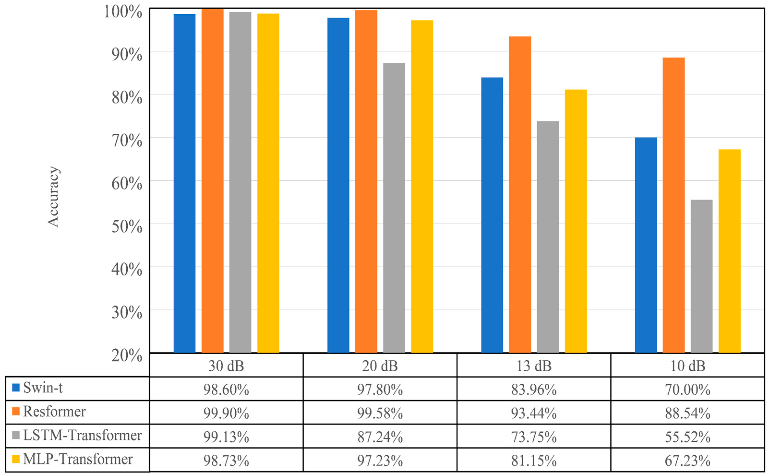
| Model | SNR | Parameter (M) | Training Time (h) | Running Time (s/Sample) | |||
|---|---|---|---|---|---|---|---|
| 30 dB | 20 dB | 13 dB | 10 dB | ||||
| Resformer | 99.90% | 99.58% | 93.44% | 88.54% | 32.2 | 2.2 | 0.636 |
| Swin-t | 98.60% | 97.80% | 83.96% | 70.00% | 19.6 | 1.1 | 0.569 |
| Swin-s | 99.48% | 98.02% | 82.77% | 66.52% | 49.6 | 2.4 | 0.938 |
| Swin-b | 99.61% | 99.16% | 76.19% | 60.49% | 87.8 | 2.1 | 0.944 |
| VGG-11 | 98.30% | 97.22% | 80.94% | 67.61% | 132.9 | 0.9 | 0.617 |
| VGG-19 | 99.58% | 99.17% | 84.69% | 73.96% | 143.7 | 1.4 | 0.808 |
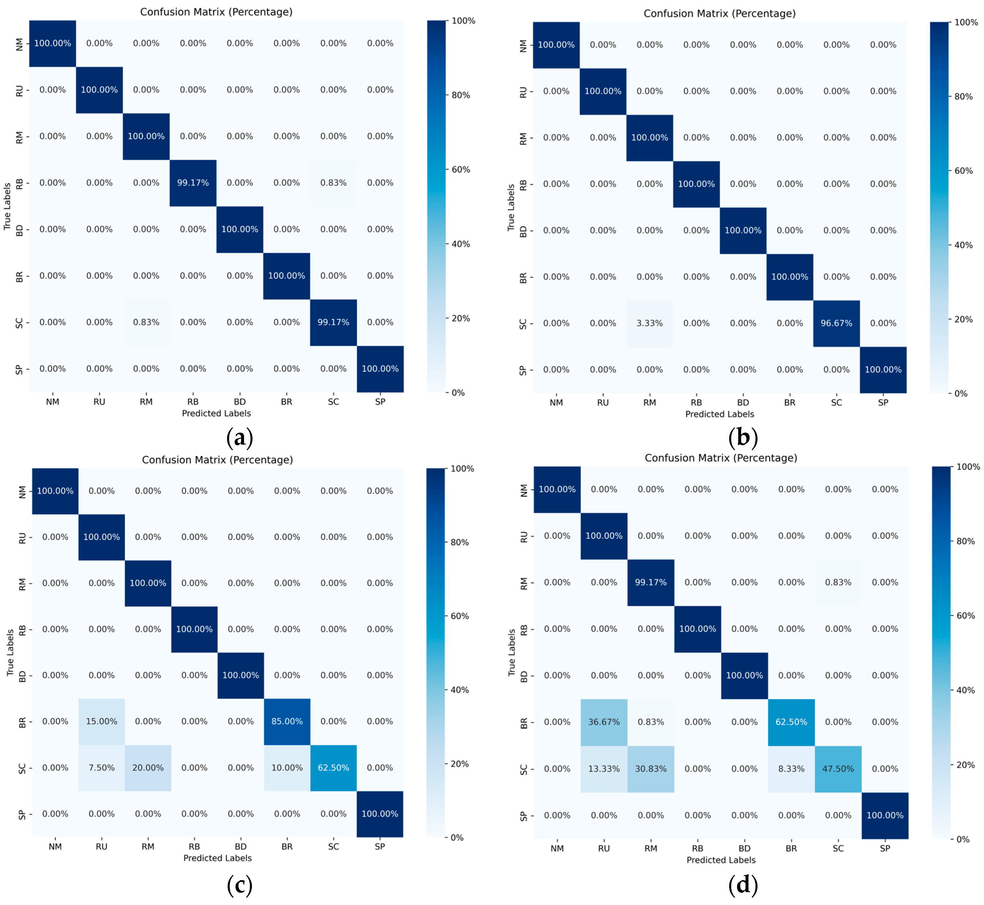
| Fault Label | 30 dB | 20 dB | ||||
|---|---|---|---|---|---|---|
| Precision | Recall | F1 Score | Precision | Recall | F1 Score | |
| NM | 1 | 1 | 1 | 1 | 1 | 1 |
| RU | 1 | 1 | 1 | 1 | 1 | 1 |
| RM | 0.992 | 1 | 0.996 | 0.968 | 1 | 0.984 |
| RB | 1 | 0.992 | 0.996 | 1 | 1 | 1 |
| BD | 1 | 1 | 1 | 1 | 1 | 1 |
| BR | 1 | 1 | 1 | 1 | 1 | 1 |
| SC | 0.992 | 0.992 | 0.992 | 1 | 0.967 | 0.983 |
| SP | 1 | 1 | 1 | 1 | 1 | 1 |
| Fault Label | 13 dB | 10 dB | ||||
|---|---|---|---|---|---|---|
| Precision | Recall | F1 Score | Precision | Recall | F1 Score | |
| NM | 1 | 1 | 1 | 1 | 1 | 1 |
| RU | 0.816 | 1 | 0.899 | 0.667 | 1 | 0.8 |
| RM | 0.83 | 1 | 0.909 | 0.758 | 0.992 | 0.860 |
| RB | 1 | 1 | 1 | 1 | 1 | 1 |
| BD | 1 | 1 | 1 | 1 | 1 | 1 |
| BR | 0.895 | 0.850 | 0.872 | 0.882 | 0.625 | 0.732 |
| SC | 1 | 0.625 | 0.769 | 0.983 | 0.475 | 0.640 |
| SP | 1 | 1 | 1 | 1 | 1 | 1 |
Disclaimer/Publisher’s Note: The statements, opinions and data contained in all publications are solely those of the individual author(s) and contributor(s) and not of MDPI and/or the editor(s). MDPI and/or the editor(s) disclaim responsibility for any injury to people or property resulting from any ideas, methods, instructions or products referred to in the content. |
© 2024 by the authors. Licensee MDPI, Basel, Switzerland. This article is an open access article distributed under the terms and conditions of the Creative Commons Attribution (CC BY) license (https://creativecommons.org/licenses/by/4.0/).
Share and Cite
Shang, Q.; Jin, T.; Chen, M. A New Cross-Domain Motor Fault Diagnosis Method Based on Bimodal Inputs. J. Mar. Sci. Eng. 2024, 12, 1304. https://doi.org/10.3390/jmse12081304
Shang Q, Jin T, Chen M. A New Cross-Domain Motor Fault Diagnosis Method Based on Bimodal Inputs. Journal of Marine Science and Engineering. 2024; 12(8):1304. https://doi.org/10.3390/jmse12081304
Chicago/Turabian StyleShang, Qianming, Tianyao Jin, and Mingsheng Chen. 2024. "A New Cross-Domain Motor Fault Diagnosis Method Based on Bimodal Inputs" Journal of Marine Science and Engineering 12, no. 8: 1304. https://doi.org/10.3390/jmse12081304
APA StyleShang, Q., Jin, T., & Chen, M. (2024). A New Cross-Domain Motor Fault Diagnosis Method Based on Bimodal Inputs. Journal of Marine Science and Engineering, 12(8), 1304. https://doi.org/10.3390/jmse12081304