
Assessing the Influence of the Benthic/Pelagic Exchange on the Nitrogen and Phosphorus Status of the Water Column, under Physical Forcings: A Modeling Study

Abstract
:1. Introduction
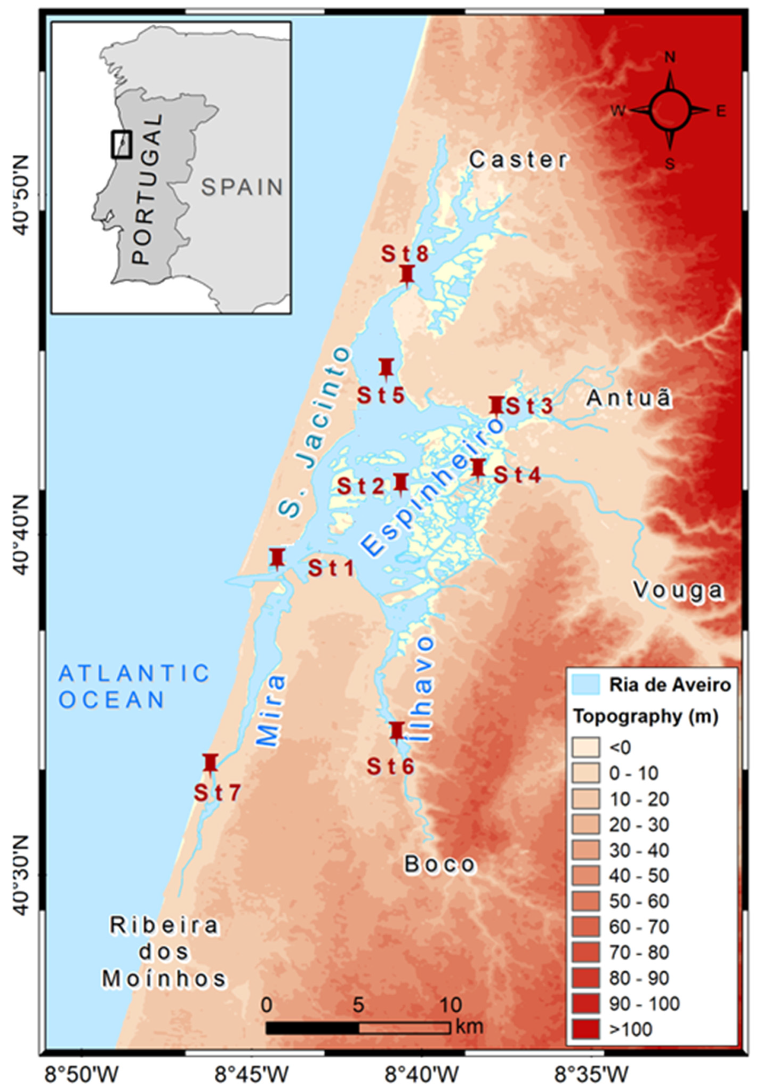
The Study Area
2. Material and Methods
2.1. The Main Model
2.2. The Pelagic Biogeochemistry Module
2.3. The Benthic Biogeochemistry Module
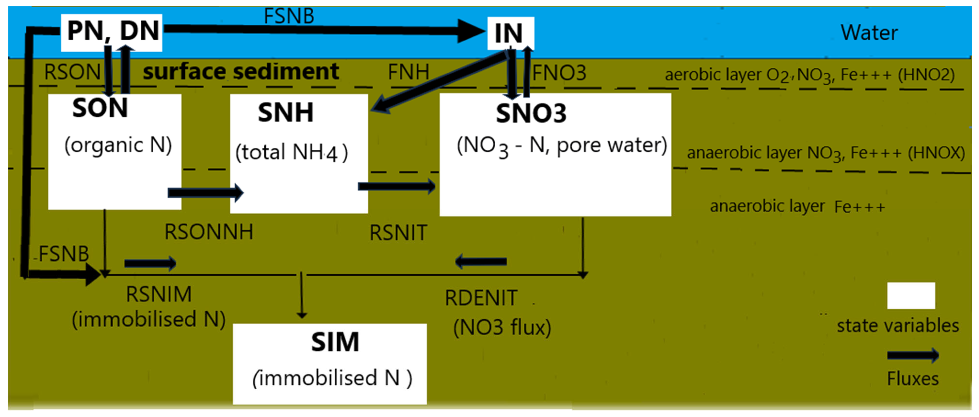
2.3.1. The Nitrogen Cycle in the Sediment Layer
- -
- SON for organic N in sediment;
- -
- SNH representing total NH4-N in sediment pore water;
- -
- SN03 indicating total NO3 in sediment;
- -
- SNIM for immobilized N in sediments.
- -
- the remaining organic N in the sediment that contributes to the SON pool;
- -
- the fraction of SON, which is mineralized into NH4;
- -
- the fraction of the settled nitrogen which is assumed to be buried into the sediment layer.
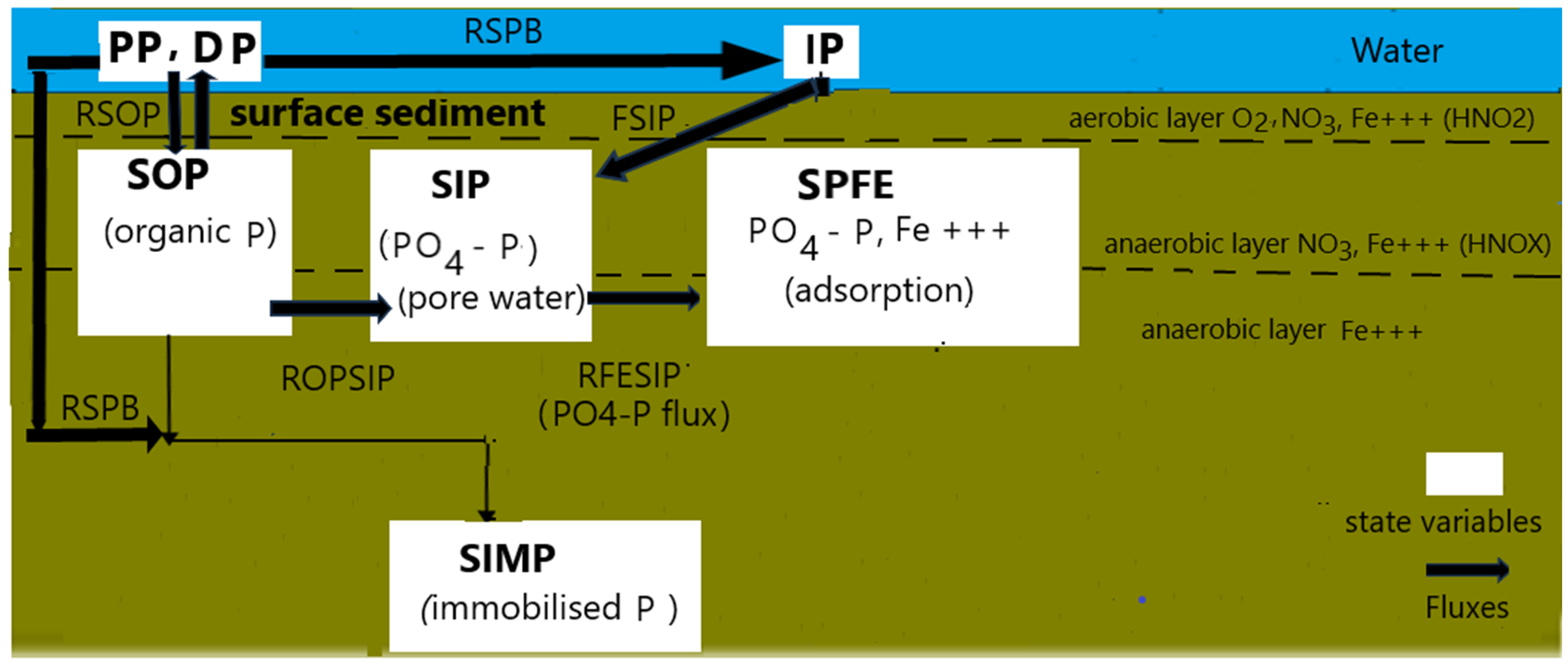
2.3.2. The Phosphorus Cycle in the Sediment Layer
- -
- SOP, which accounts for the organic P in sediment, which is mineralized into PO4. The exchanges of SOP through the sediment surface occur through sedimentation of algae and detritus P. A fraction of the settled SOP can be as well mineralized into PO4 on the sediment surface;
- -
- SIP, which accounts for the total PO4-P in sediment pore water;
- -
- SPFE, which accounts for the sediment PO4-P adsorbed to Fe+++; and SPIM, which accounts for the immobile P in the sediment.
- -
- the remaining organic in the sediment P which flows into the organic P pool;
- -
- the fraction of the organic P in the sediment, SOP, which is mineralized into PO4, and is released into the pore water pool of PO4 (SIP);
- -
- the flux of PO4 between sediment and water which accounts for the sorption and desorption of PO4 to Fe+++.
2.4. The Statistical Tools
2.4.1. Baseline Metrics
- MAPE (Mean Absolute Percentage Error): It measures the average absolute percentage difference between predicted values and observed values/mean values. It is calculated as the average of the absolute differences between predicted and observed values, divided by the observed values, and multiplied by 100.
- RMSE (Root Mean Squared Error): It measures the square root of the average of the squared differences between predicted and observed values. It provides an overall measure of the model’s error, with higher values indicating larger errors:
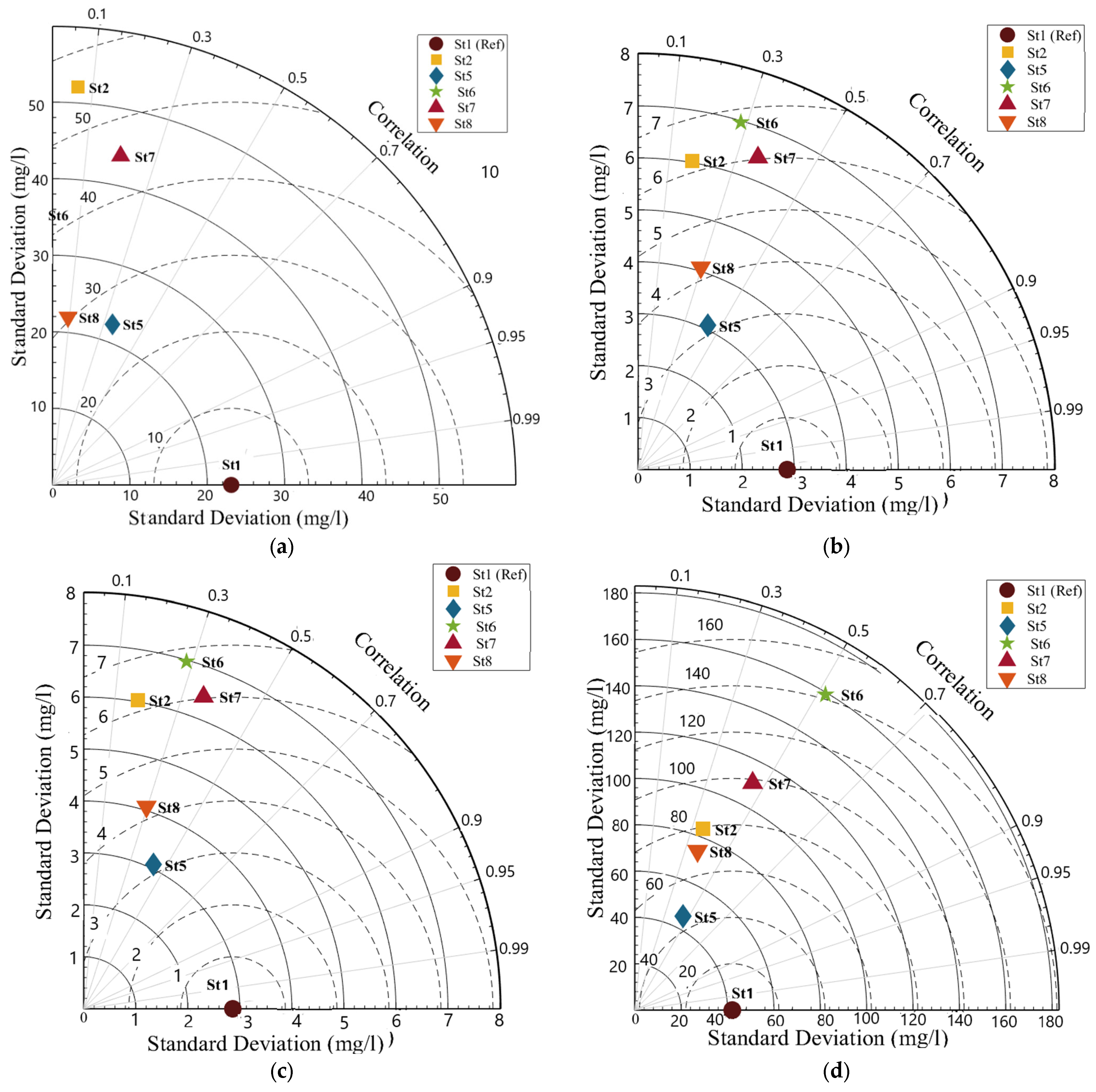
2.4.2. Taylor Diagrams
3. Results
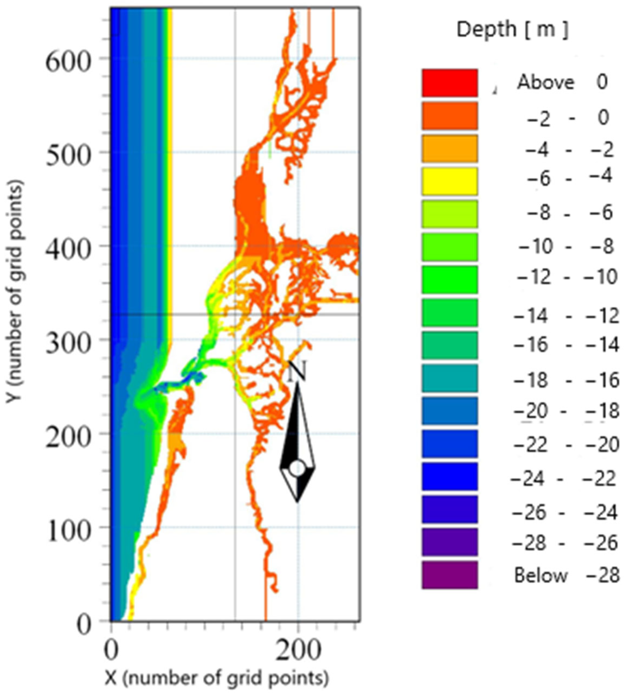
3.1. The Model Setup and Application
Model Validation
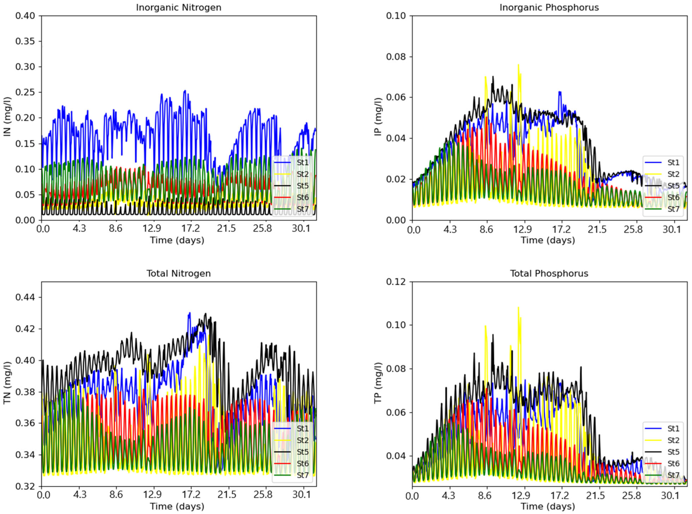
3.2. The Influence of the Physical Forcing on the Nitrogen and Phosphorus State of the Water Column
3.2.1. The River Flow Influence
3.2.2. The Water Temperature Influence
3.2.3. The Salinity Influence
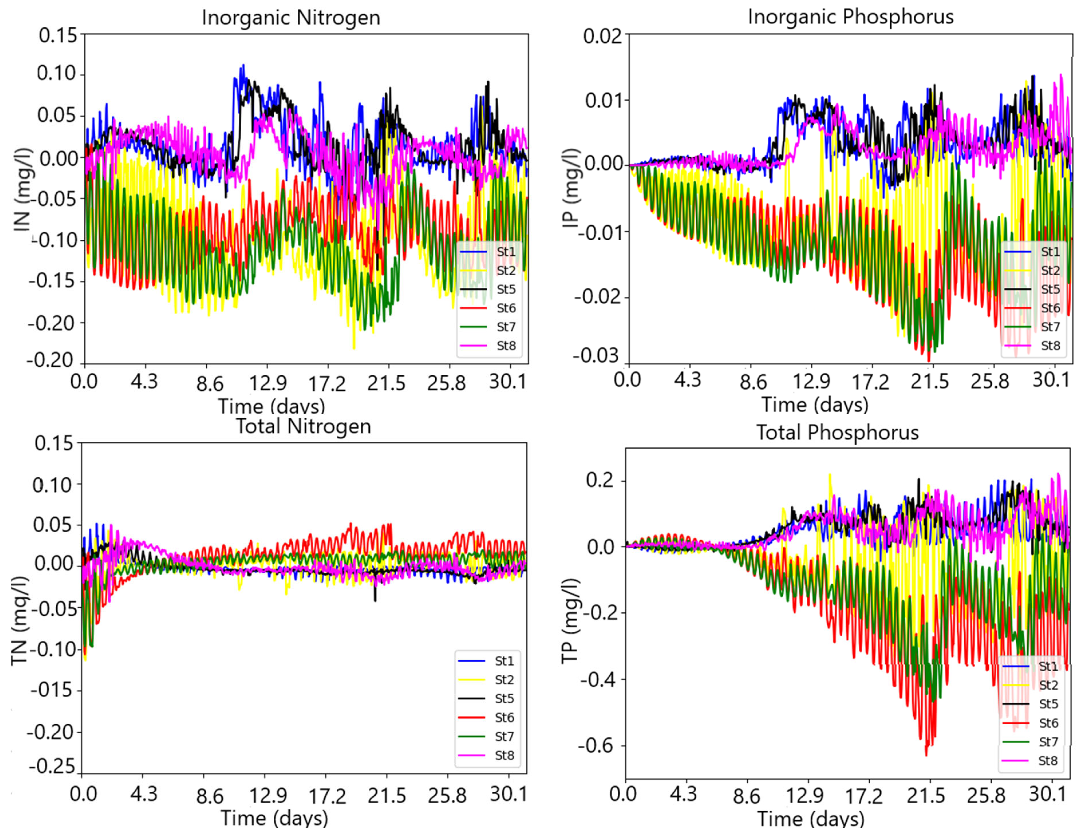
3.3. Simulating the Nitrogen and Phosphorus State of the Water Column under River Flow and Nutrient Pulses
4. Discussion and Conclusions
Supplementary Materials
Funding
Institutional Review Board Statement
Informed Consent Statement
Data Availability Statement
Conflicts of Interest
References
- Jilbert, T.S. Understanding mud: The importance of sediment biogeochemistry. Geologi 2016, 68, 80–87. [Google Scholar]
- Canfield, D.E.; Thamdrup, B.; Kristensen, E. Aquatic Geomicrobiology; Elsevier: Amsterdam, The Netherlands, 2005; 640p. [Google Scholar]
- Lessin, G.; Artioli, Y.; Almroth-Rosell, E.; Blackford, J.C.; Dale, A.; Glud, R.; Middelburg, J.J.; Pastres, R.; Queiros, A.M.; Rabouille, C.; et al. Modelling marine sediment biogeochemical: Current knowledge gaps, challenges and some methodological advice for advancement. Front. Mar. Sci. 2018, 5, 19. [Google Scholar] [CrossRef]
- Arndt, S.; Jørgensen, B.; LaRowe, D.; Middelburg, J.; Pancost, R.; Regnier, P. Quantifying the degradation of organic matter in marine sediments: A review and synthesis. Earth-Sci. Rev. 2013, 123, 53–86. [Google Scholar] [CrossRef]
- Sin, S.; Banerjee, A.; Rakshit, N.; Raman, A.; Bhadury, P.; Ray, S. Importance of benthic-pelagic coupling in food-web interactions of Kakinada Bay, India. Ecol. Inform. 2021, 61, 101208. [Google Scholar] [CrossRef]
- Sohma, A.; Imada, R.; Nishikawa, T.; Shibuki, H. Modeling the life cycle of four types of phytoplankton and their bloom mechanisms in a benthic-pelagic coupled ecosystem. Ecol. Model. 2022, 467, 109882. [Google Scholar] [CrossRef]
- Yakubov, S.; Wallhead, P.; Protsenko, E.; Yakushev, E.; Pakhomova, S.; Brix, H. A 1-Dimensional Sympagic–Pelagic–Benthic Transport Model (SPBM): Coupled Simulation of Ice, Water Column, and Sediment Biogeochemistry, Suitable for Arctic Applications. Water 2019, 11, 1582. [Google Scholar] [CrossRef]
- Boudreau, B.P. Diagenetic Models and Their Implementation; Springer: Berlin/Heidelberg, Germany, 1997. [Google Scholar]
- Berner, R.A. Early Diagenesis: A Theoretical Approach; Princeton University Press: Princeton, NJ, USA, 1980; 241p. [Google Scholar]
- Lohse, L.; Malschaert, J.; Slomp, C.; Helder, W.; Van Raaphorst, W. Nitrogen cycling in North Sea sediments: Interaction of denitrification and nitrification in offshore and coastal areas. Mar. Ecol. Prog. Ser. 1993, 101, 283–296. [Google Scholar] [CrossRef]
- Xia, X.; Dong, J.; Wang, M.; Xie, H.; Xia, N.; Li, H.; Zhang, X.; Mou, X.; Wen, J.; Bao, Y. Effect of water-sediment regulation of the Xiaolangdi Reservoir on the concentrations, characteristics, and fluxes of suspended sediment and organic carbon in the Yellow River. Sci. Total Environ. 2016, 571, 487–497. [Google Scholar] [CrossRef]
- Wijsman, J.; Herman, P.; Gomoiu, M. Spatial distribution in sediment characteristics and benthic activity on the northwestern Black Sea shelf. Mar. Ecol. 1999, 181, 25–39. [Google Scholar] [CrossRef]
- Boynton, W.; Kemp, W. Nutrient regeneration and oxygen consumption by sediments along an estuarine salinity gradient. Mar. Ecol. Prog. Ser. 1985, 23, 45–55. [Google Scholar] [CrossRef]
- Sweerts, J.-P. Oxygen Consumption, Mineralization and Nitrogen Cycling at the Sediment–Water Interface of North Temperate Lakes. Ph.D. Thesis, University of Groningen, Groningen, The Netherlands, 1990; 136p. [Google Scholar]
- Sweerts, J.-P.R.A.; St Louis, V.; Cappenberg, T.E. Oxygen concentration profiles and exchange in sediment cores with circulated overlying water. Freshw. Biol. 1990, 21, 401–409. [Google Scholar] [CrossRef]
- Sweerts, J.-P.R.A.; Bar-Gilissen, M.-J.; Coruelese, A.A.; Cappenberg, T.E. Oxygen-consuming processes at the profundal and littoral sediment-water interface of a small mesoeutrophic lake (Lake Vechten, The Netherlands). Limnol. Oceaonogr. 1991, 36, 1124–1133. [Google Scholar] [CrossRef]
- Cai, W.J.; Sayles, F.L. Oxygen penetration depths and fluxes in marine sediments. Mar. Chem. 1996, 52, 123–131. [Google Scholar] [CrossRef]
- Soetaert, K.; Herman, P.; Middelburg, J. A model of early diagenesis processes from the shelf to abyssal depths. Geochim. Cosmochim. Acta 1996, 60, 1019–1040. [Google Scholar] [CrossRef]
- Soetaert, K.; Middelburg, J. Modeling eutrophication and oligotrophication of shallow-water marine systems: The importance of sediments under stratified and well-mixed conditions. Hydrobiologia 2009, 629, 239–254. [Google Scholar] [CrossRef]
- Soetaert, K.; Middelburg, J.; Herman, P.; Buis, K. On the coupling of benthic and pelagic biogeochemical models. Earth Sci. Rev. 2000, 51, 173–201. [Google Scholar] [CrossRef]
- Hülse, D.; Arndt, S.; Wilson, J.; Munhoven, G.; Ridgwell, A. Understanding the causes and consequences of past marine carbon cycling variability through models. Earth Sci. Rev. 2017, 171, 349–382. [Google Scholar] [CrossRef]
- Moriarty, J.; Harris, C.; Fennel, K.; Friedrichs, M.; Kehui, X.; Rabouille, C. The roles of resuspension, diffusion and biogeochemical processes on oxygen dynamics offshore of the Rhône River, France: A numerical modeling study. Biogeosciences 2017, 14, 1919–1946. [Google Scholar] [CrossRef]
- Laurent, A.; Fennel, K.; Wilson, R.; Lehrter, J.; Devereux, R. Parameterization of biogeochemical sediment-water fluxes using in situ measurements and a diagenetic model. Biogeosciences 2016, 13, 77–94. [Google Scholar] [CrossRef]
- Wilson, R.; Fennel, K.; Paul, J. Simulating sediment–water exchange of nutrients and oxygen: A comparative assessment of models against mesocosm observations. Cont. Shelf Res. 2013, 63, 69–84. [Google Scholar] [CrossRef]
- Baretta, J.; Ebenhöh, W.; Ruardij, P. The European regional seas ecosystem model, a complex marine ecosystem model. Neth. J. Sea Res. 2005, 33, 233–246. [Google Scholar] [CrossRef]
- Brigolin, D.; Lovato, T.; Rubino, A.; Pastres, R. Coupling early-diagenesis and pelagic biogeochemical models for estimating the seasonal variability of N and P fluxes at the sediment-water interface: Application to the northwestern Adriatic coastal zone. J. Mar. Syst. 2011, 87, 239–255. [Google Scholar] [CrossRef]
- Testa, J.; Kemp, W. Hypoxia-induced shifts in nitrogen and phosphorus cycling in Chesapeake Bay. Limnol. Oceanogr. 2012, 57, 835–850. [Google Scholar] [CrossRef]
- Fennel, K.; Brady, D.; DiToro, D.; Fulweiler, R.; Gardner, W.; McCarthy, M.; Rao, A.; Seitzinger, S.; Thouvenot-Korppoo, M.; Tobias, C. Modelling denitrification in aquatic sediments. Biogeochemical 2009, 93, 159–178. [Google Scholar] [CrossRef]
- Testa, J.; Brady, D.; Toro, D.; Boynton, W.; Cornwell, J.; Kemp, W. Sediment flux modeling: Nitrogen, phosphorus and silica cycles. Estuar. Coast. Shelf Sci. 2013, 131, 245–263. [Google Scholar] [CrossRef]
- Testa, J.; Li, Y.; Lee, Y.; Li, M.; Brady, D.; Di Toro, D.; Kemp, W. Quantifying the effects of nutrient loading on dissolved O2 cycling and hypoxia in Chesapeake Bay using a coupled hydrodynamic–biogeochemical model. J. Mar. Syst. 2013, 139, 139–158. [Google Scholar] [CrossRef]
- Testa, J.; Kemp, W. Spatial and temporal patterns in winter-spring oxygen depletion in Chesapeake Bay bottom waters. Estuar. Coasts 2014, 37, 1432–1448. [Google Scholar] [CrossRef]
- Paraska, D.; Hipsey, M.; Salmon, S. Sediment diagenesis models: Review of approaches, challenges and opportunities. Environ. Model. Softw. 2014, 61, 297–325. [Google Scholar] [CrossRef]
- Bruggemann, J.; Bolding, K. A general framework for aquatic biogeochemical models. Environ. Model. Softw. 2014, 61, 249–265. [Google Scholar] [CrossRef]
- Gehlen, M.; Barciela, R.; Bertino, L.; Brasseur, P.; Butenschön, M.; Chai, F.; Crise, A.; Drillet, Y.; Ford, D.; Lavoie, D. Building the capacity for forecasting marine biogeochemistry and ecosystems: Recent advances and future developments. J. Oper. Oceanogr. 2015, 8 (Suppl. S1), s168–s187. [Google Scholar] [CrossRef]
- Ford, D.; Kay, S.; McEwan, R.; Totterdell, I.; Gehlen, M. Marine Biogeochemical Modelling and Data Assimilation for Operational Forecasting, Reanalysis, and Climate Research. In New Frontiers in Operational Oceanography; 2018; pp. 625–652. Available online: https://diginole.lib.fsu.edu/islandora/object/fsu%3A602120 (accessed on 1 July 2024).
- Akbarzadeh, Z.; Laverman, A.; Rezanezhad, F.; Raimonet, M.; Viollier, E.; Shafei, B.; Van Cappellen, P. Benthic nitrite exchanges in the Seine River (France) An early diagenetic modeling analysis. Sci. Total Environ. 2018, 628–629, 580–593. [Google Scholar] [CrossRef] [PubMed]
- Billen, G.; Lancelot, C. Modelling benthic nitrogen cycling in temperate coastal ecosystems. In Nitrogen Cycling in Coastal Marine Environments; Blackburn, T.H., Sorensen, J., Eds.; Wiley and Sons: New York, NY, USA, 1988; pp. 341–378. [Google Scholar]
- Berg, P.; Rysgaard, S.; Thamdrup, B. General dynamic modelling of early diagenesis and nutrient cycling, Applied to an Arctic marine sediment. J. Am. Sci. 2003, 303, 905–955. [Google Scholar] [CrossRef]
- Wijsman, J.; Herman, P.; Middelburg, J.; Soetaert, K. A model for early diagenesis processes in sediments of the continental shelf of the Black Sea. Estuar. Coast. Shelf Sci. 2002, 54, 403–421. [Google Scholar] [CrossRef]
- Dias, J.M. Contribution to the Study of the Ria de Aveiro Hydrodynamics. Ph.D. Thesis, Universidade de Aveiro, Aveiro, Portugal, 2001; 288p. [Google Scholar]
- Dias, J.; Lopes, J.; Dekeyser, I. Hydrological characterisation of Ria de Aveiro lagoon, Portugal, in early summer. Oceanol. Acta 1999, 22, 473–485. [Google Scholar] [CrossRef]
- Moreira, M.H.; Queiroga, H.; Machado, M.M.; Cunha, M.R. Environmental gradients in a southern estuarine system: Ria de Aveiro, Portugal, implication for soft bottom macrofauna colonization. Aquat. Ecol. 1993, 27, 465–482. [Google Scholar] [CrossRef]
- Almeida, M.A.; Cunha, M.A.; Alcântara, F. Relationship of bacterioplankton production with primary production and respiration in a shallow estuarine system, Ria de Aveiro, NW Portugal. Microbiol. Res. 2005, 160, 315–328. [Google Scholar] [CrossRef] [PubMed]
- Lopes, C.B.; Lillebø, A.I.; Dias, J.M.; Pereira, E.; Vale, C.; Duarte, A.C. Nutrient dynamics and seasonal succession of phytoplankton assemblages in a Southern European Estuary: Ria de Aveiro, Portugal. Estuar. Coast. Shelf Sci. 2007, 71, 480–490. [Google Scholar] [CrossRef]
- Génio, L.; Sousa, A.; Vaz, N.; Dias, J.M.; Barroso, C. Effect of low salinity on the survival of recently hatched veliger of Nassarius reticulatus (L.) in estuarine habitats: A case study of Ria de Aveiro. J. Sea Res. 2008, 59, 133–143. [Google Scholar] [CrossRef]
- Lopes, J.F.; Almeida, M.A.; Cunha, M.A. Modelling the ecological patterns of a temperate lagoon in a very wet spring season. Ecol. Model. 2010, 221, 2302–2322. [Google Scholar] [CrossRef]
- Lopes, J.F.; Vaz, N.; Ferreira, J.A.; Dias, J.M. Assessing the state of the lower level of the trophic web of a temperate lagoon, in situations of light or nutrient stress: A modelling study. Ecol. Model. 2015, 313, 59–76. [Google Scholar] [CrossRef]
- ModelRia. Modelação da Qualidade da Água na Laguna da Ria de Aveiro; Final Report; Universidade de Aveiro-Centro das Zonas Costeiras e do Mar, Instituto Superior Técnico—Centro de Ambiente e Tecnologias Marítimos and Hidromod: Aveiro, Portugal, 2023. [Google Scholar]
- Serôdio, J.; Paterson, D.M.; Méléder, V.; Vyverman, W. Advances and challenges in microphytobenthos research: From cell biology to coastal ecosystem function. Front. Mar. Sci. 2020, 7, 608729. [Google Scholar] [CrossRef]
- MIKE 3 Flow Model. Hydrodynamic Module. User Guide. Scientific Documentation. 2017. Available online: https://manuals.mikepoweredbydhi.help/2017/Coast_and_Sea/MIKE_FM_HD_3D.pdf (accessed on 1 July 2024).
- MIKE 3 Flow Model ECO Lab Module. Eutrophication Model Incl. Sediment and Benthic Vegetation. User Guide. Scientific Documentation. 2017. Available online: https://www.dhigroup.com/technologies/mikepoweredbydhi/mike-eco-lab (accessed on 1 July 2017).
- Williams, P.J.L. Aspects of dissolved organic material in sea water. In Chemical Oceanography; Chapter 1; Riley, J.P., Skirrow, G., Eds.; Academic Press: New York, NY, USA, 1975; pp. 301–363. [Google Scholar]
- Nyholm, N. A simulation model for phytoplankton growth and nutrient cycling in eutrophic, shallow lakes. Ecol. Model. 1978, 4, 279–310. [Google Scholar] [CrossRef]
- Henriksen, K. Measurement of in situ rates of nitrification in sediment. Microb. Ecol. 1981, 6, 329–337. [Google Scholar] [CrossRef] [PubMed]
- Jørgensen, B.B. Mineralization of organic matter in the seabed—Role of sulphate reduction. Nature 1982, 296, 643–645. [Google Scholar] [CrossRef]
- Henriksen, K.; Hansen, J.I.; Blackburn, T.H. Rates of nitrification, distribution of nitrifying bacteria, and nitrate fluxes in different types of sediments from Danish waters. Mar. Biol. 1981, 61, 299–304. [Google Scholar] [CrossRef]
- Henriksen, K.; Kemp, W. Nitrification in estuarine and coastal marine sediments. In Nitrogen Cycling in Coastal Marine Environments; Blackburn, T.H., Sorensen, J., Eds.; John Wiley and Sons, Inc.: New York, NY, USA, 1988; pp. 201–249. [Google Scholar]
- Nixon, S.; Arnmerman, J.; Atkinson, L.; Berounsky, V.; Billen, G.; Boicourt, W.; Boynton, W.; Church, T.; DiToro, D.; Ehgren, R.; et al. The fate of nitrogen and phosphorus at the land-sea margin of the North Atlantic Ocean. Biogeochemical 1996, 35, 141–180. [Google Scholar] [CrossRef]
- Taylor, K.E. Summarizing multiple aspects of model performance in a single diagram. J. Geophys. Res. 2001, 106, 7183–7192. [Google Scholar] [CrossRef]
- Vaz, N.; Dias, J.M. Hydrographic characterization of an estuarine tidal channel. J. Mar. Syst. 2008, 70, 168–181. [Google Scholar] [CrossRef]
- Hayn, M.; Howarth, R.; Marino, R.; Ganju, N.; Berg, P.; Foreman, K.; Giblin, A.; McGlathery, K. Exchange of Nitrogen and Phosphorus Between a Shallow Lagoon and Coastal Waters. Estuaries Coasts 2014, 37 (Suppl. S1), 63–73. [Google Scholar] [CrossRef]
- Blackburn, T.; Henriksen, K. Nitrogen cycling in different types of sediments from Danish Waters. Limnol. Oceanogr. 1983, 28, 477–493. [Google Scholar] [CrossRef]
- Bocci, M.; Coffaro, G.; Bendoricchio, G. Modelling biomass and nutrient dynamics in eelgrass (Zostera marina): Applications to Lagoon of Venice (Italy) and Øresund (Denmark). Ecol. Model. 1997, 102, 67–80. [Google Scholar] [CrossRef]
- Lomstein, B.; Blackburn, T.H.; Blackburn, N.D.; Lomstein, E.; Hansen, L.S.; Therkildsen, M.S.; King, G.M.; Holmer, M. Decomposition of Organic Nitrogen in Marine Sediments. Marine Research from the Danish Environmental Protection Agency. 1995. 58p. Available online: https://www2.mst.dk/Udgiv/publikationer/1995/87-7810-489-0/pdf/87-7810-489-0.pdf (accessed on 1 July 2024).
- Bendoricchio, G.; Coffaro, G.; De Marchi, C. A trophic model for Ulva rigida in the Lagoon of Venice. Ecol. Model. 1994, 75–76, 485–496. [Google Scholar] [CrossRef]
- Ruadij, P.; Raaphorst, W. Benthic nutrient regeneration in the ERSEM ecosystem model of the North Sea. Neth. J. Sea Res. 1995, 33, 453–483. [Google Scholar] [CrossRef]
- Coffaro, G.; Bocci, M. Resources competition between Ulva rigida and Zostera marina: A quantitative approach applied to the Lagoon of Venice. Ecol. Model. 1997, 102, 81–95. [Google Scholar] [CrossRef]
- Iziumi, H.; Hattori, A. Growth, and organic production of eelgrass (Zostera marina) in temperate waters of the pacific coast of Japan. III The kinetics of nitrogen uptake. Aquat. Bot. 1982, 12, 245–256. [Google Scholar] [CrossRef]
- Jensen, H.; Mortensen, P.; Andersen, F.Ø.; Rasmussen, E.K.; Jensen, A. Phosphorus cycling in coastal marine sediment. Limnol. Oceanogr. 1995, 40, 908–917. [Google Scholar] [CrossRef]
- Mortensen, P.; Jensen, H.; Rasmussen, E.K.; Østergaard, P. Phosphorus Turnover in the Sediment in Aarhus Bay. Marine Research from the Danish Environmental Protection Agency. 1992. Cited by Mike 3. Available online: https://manuals.mikepoweredbydhi.help/2017/MIKE_3.htm (accessed on 1 July 2024).
- Jacobsen, O. Sorption, adsorption and chemosorption of phosphate by Danish Lake sediments. Vatten 1978, 4, 230–241. [Google Scholar]
- Jacobsen, O. Sorption of phosphate by Danish Lake Sediments. Vatten 1997, 3, 290–298. [Google Scholar]
- Gundresen, K.J.; Glud, R.N.; Jørgensen, B.B. Oxygen Turnover of the Seabed. Marine Research from the Danish Environmental Protection Agency. 1995. 57p; Cited by Mike 3. Available online: https://manuals.mikepoweredbydhi.help/2017/MIKE_3.htm (accessed on 1 July 2024).
- Sweerts, J.-P.; Carol, A.; Rudd, J.; Hesslein, R.; Cappenberg, T. Similarity of whole-sediment molecular diffusion coefficients in freshwater sediments of low and high porosity. Limnol. Oceanogr. 1991, 36, 336–341. [Google Scholar] [CrossRef]
- Windolf, J.; Jeppesen, E.; Jensen, J.; Kristensen, P. Modelling of seasonal variation in nitrogen retention and in-lake concentration: A four-year mass balance study in 16 shallow Danish Lakes. Biogeochemistery 1996, 33, 25–44. [Google Scholar] [CrossRef]


| Boundaries | Discharge (m3/s) | Salinity (PSU) | Water Temp. (°C) | N (mg/L) | P (mg/L) | DO (mg/L) |
|---|---|---|---|---|---|---|
| Vouga river | 50–300 | 0 | 13–19 | 1.4–3.7 | 0.1–0.2 | 8.0–12.0 |
| Antuã river | 20–50 | 0 | 1.3–23 | 4.0–12 | 0.1–1.2 | 6.5–9.5 |
| Mira | 0–10 | 0 | 16–23 | 1.5–5.0 | 0.1–0.6 | 8.0–9.2 |
| Other rivers | 0–10 | 0 | 13–22 | 1.0–10 | 0.1–0.9 | 6.5–9.0 |
| Ocean | - | 6–34 | 13–22 | 0.1–1.3 | 0.03–0.06 | 8.0–11.0 |
| St1 | St2 | St3 | St4 | St5 | St6 | St7 | St8 | |
|---|---|---|---|---|---|---|---|---|
| TN (mg N/L) | 0.03–0.2 | 0.27–0.32 | 0.31–0.65 | 0.26–0.32 | 0.10–0.20 | 0.37–0.60 | 0.37–0.60 | 0.10–0.60 |
| TP (mg P/L) | 0.03–0.03 | 0.03–0.03 | 0.03–0.03 | 0.03–0.03 | 0.03–0.03 | 0.05–0.07 | 0.05–0.08 | 0.05–0.08 |
| PC (mg/L) | 0.10–0.20 | 0.10–0.20 | 0.10–0.30 | 0.10–0.30 | 0.10–0.20 | 0.10–0.20 | 0.10–0.30 | 0.10–0.30 |
| Chl (mg/L) | 2–3 | 1–1 | 4–6 | 4–5 | 2–4 | 2–6 | 2–6 | 2–6 |
| DO (mg/L) | 9–10 | 9–10 | 9–9 | 9–10 | 9–10 | 8–10 | 8–10 | 8–10 |
| St1 | St2 | St3 | St4 | St5 | St6 | St7 | St8 | |
|---|---|---|---|---|---|---|---|---|
| TN RM (mg N/L) | 7.41 × 10⁻² | 5.24 × 10⁻² | 7.85 × 10⁻² | 2.76 × 10⁻² | 9.44 × 10⁻² | 5.42 × 10⁻² | 1.45 × 10⁻¹ | 2.12 × 10⁻¹ |
| TN MP (%) | 20 | 15 | 20 | 9 | 24 | 16 | 42 | 51 |
| IN RM (mg N/L) | 5.93 × 10⁻² | 1.31 × 10⁻¹ | 1.21 × 10⁻¹ | 1.46 × 10⁻¹ | 7.79 × 10⁻² | 1.14 × 10⁻¹ | 1.06 × 10⁻¹ | 1.43 × 10⁻¹ |
| IN MP (%) | 15 | 33 | 30 | 35 | 20 | 29 | 25 | 36 |
| TP RM (mg P/L) | 9.09 × 10⁻³ | 4.53 × 10⁻³ | 6.64 × 10⁻³ | 4.41 × 10⁻³ | 9.47 × 10⁻³ | 3.13 × 10⁻³ | 3.33 × 10⁻³ | 4.02 × 10⁻³ |
| TP MP (%) | 30 | 15 | 22 | 15 | 32 | 52 | 56 | 67 |
| IP RM (mg P/L) | 8.11 × 10⁻³ | 1.35 × 10⁻² | 1.45 × 10⁻³ | 1.64 × 10⁻³ | 1.08 × 10⁻³ | 5.25 × 10⁻³ | 4.48 × 10⁻³ | 3.92 × 10⁻³ |
| IP MP (%) | 27 | 45 | 5 | 6 | 4 | 18 | 15 | 13 |
| St1 | St2 | St3 | St4 | St5 | St6 | St7 | St8 | |
|---|---|---|---|---|---|---|---|---|
| TN RM (mg N/L) | 5.34 × 10⁻² | 2.17 × 10⁻² | 1.22 × 10⁻¹ | 5.28 × 10⁻¹ | 4.53 × 10⁻² | 1.59 × 10⁻² | 1.14 × 10⁻¹ | 9.16 × 10⁻² |
| TN MP (%) | 54 | 22 | 20 | 6 | 45 | 16 | 57 | 46 |
| IN RM (mg N/L) | 2.65 × 10⁻² | 4.84 × 10⁻² | 1.48 × 10⁻¹ | 5.48 × 10⁻¹ | 3.97 × 10⁻² | 4.61 × 10⁻² | 1.44 × 10⁻¹ | 1.33 × 10⁻¹ |
| IN MP (%) | 27 | 49 | 25 | 6 | 40 | 47 | 71 | 65 |
| TP RM (mg P/L) | 2.68 × 10⁻² | 7.45 × 10⁻³ | 5.73 × 10⁻³ | 1.37 × 10⁻² | 2.09 × 10⁻² | 1.03 × 10⁻² | 8.65 × 10⁻³ | 1.64 × 10⁻² |
| TP MP (%) | 67 | 19 | 15 | 19 | 52 | 26 | 21 | 41 |
| IP RM (mg P/L) | 1.82 × 10⁻² | 3.27 × 10⁻² | 3.53 × 10⁻² | 4.78 × 10⁻² | 2.65 × 10⁻² | 3.79 × 10⁻² | 2.93 × 10⁻² | 2.35 × 10⁻² |
| IP MP (%) | 46 | 82 | 88 | 64 | 53 | 63 | 73 | 59 |
Disclaimer/Publisher’s Note: The statements, opinions and data contained in all publications are solely those of the individual author(s) and contributor(s) and not of MDPI and/or the editor(s). MDPI and/or the editor(s) disclaim responsibility for any injury to people or property resulting from any ideas, methods, instructions or products referred to in the content. |
© 2024 by the author. Licensee MDPI, Basel, Switzerland. This article is an open access article distributed under the terms and conditions of the Creative Commons Attribution (CC BY) license (https://creativecommons.org/licenses/by/4.0/).
Share and Cite
Lopes, J.F. Assessing the Influence of the Benthic/Pelagic Exchange on the Nitrogen and Phosphorus Status of the Water Column, under Physical Forcings: A Modeling Study. J. Mar. Sci. Eng. 2024, 12, 1310. https://doi.org/10.3390/jmse12081310
Lopes JF. Assessing the Influence of the Benthic/Pelagic Exchange on the Nitrogen and Phosphorus Status of the Water Column, under Physical Forcings: A Modeling Study. Journal of Marine Science and Engineering. 2024; 12(8):1310. https://doi.org/10.3390/jmse12081310
Chicago/Turabian StyleLopes, José Fortes. 2024. "Assessing the Influence of the Benthic/Pelagic Exchange on the Nitrogen and Phosphorus Status of the Water Column, under Physical Forcings: A Modeling Study" Journal of Marine Science and Engineering 12, no. 8: 1310. https://doi.org/10.3390/jmse12081310