Investigation on Calm Water Resistance of Wind Turbine Installation Vessels with a Type of T-BOW

Abstract

Given the typical characteristics of self-propulsion and jack-up wind turbine installation vessels (WTIVs), including their full and blunt hull form and complex appendages, this paper combines the model test method with the RANS-based CFD numerical prediction method to experimentally and numerically study the resistance of the optimized hull at different spudcan retraction positions. The calm water resistance components and their mechanisms of WTIVs based on T-BOW were obtained. Furthermore, using the multivariate nonlinear least squares method, an empirical formula for rapid resistance estimation based on the Holtrop method was derived, and its prediction accuracy and applicability were validated with a full-scale ship case. This study indicates that the primary resistance components of such low-speed vessels are viscous pressure resistance, followed by frictional resistance and wave-making resistance. Notably, the spudcan retraction well area, as a unique appendage of WTIVs, exhibits a significant “moonpool additional resistance” effect. Different spudcan retraction positions affect the total calm water resistance by approximately 20% to 30%. Therefore, in the resistance optimization design of WTIVs, special attention should be paid to the matching design of the spudcan structure and the hull shell plate lines in the spudcan retraction well area.

1. Introduction

Wind turbine installation vessels (WTIVs), as the main equipment for Wind Turbine Generator (WTG) deployment, have been developing towards large-scale, integrated operation modes of transportation and installation in recent years. The old-generation WTIV is a self-elevating non self-propelled installation platform suitable for coastal shallow water operation. The new generation self-propelled WTIV has stronger dynamic positioning capabilities, and the main hull has evolved from a square barge structure to a streamlined hull form with better resistance performance. While reducing the overall installed power and fuel consumption during operation, it greatly improves the efficiency of ship operations and environmental sustainability. Figure 1 illustrates the design differences between these two generations of vessels.

This paper examines the T-type bow (T-BOW) as a new type of bow structure for WTIVs, as shown in Figure 1b, which represents a significant advancement in naval architecture and which is tailored to meet the operational demands and technical specification of contemporary WTIVs. The design considerations include the following:

(1)

Ship general layout optimization: Given that the majority of the operational time for WTIVs is spent in elevated conditions, it is crucial to maximize the platform’s anti-overturning stability and the working area on the main deck during this state. Consequently, the legs of the WTIV are typically positioned as far towards the bow and stern as possible. Additionally, within the limited available space, the leg and spudcans must be accommodated at the bottom and along the sides of the vessel.

(2)

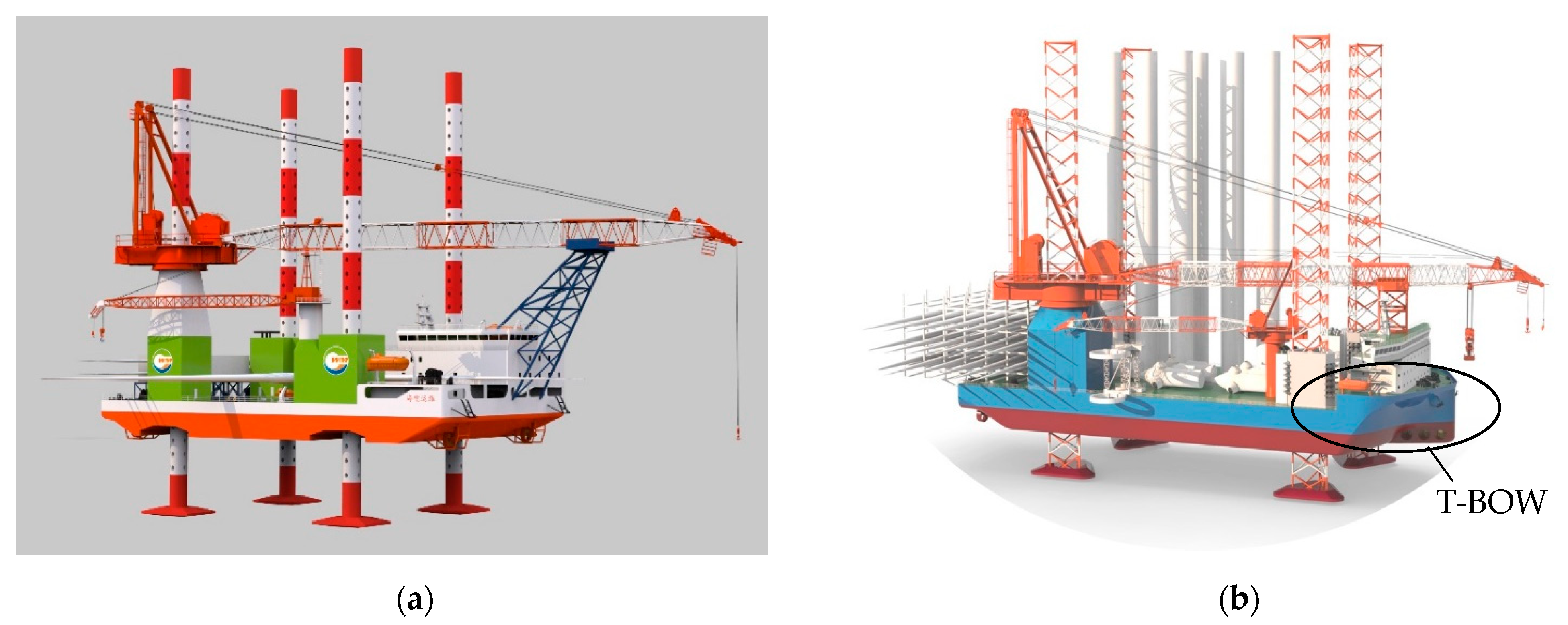
Ship main dimension optimization: Given the importance of the vessel’s DP capabilities, precise control over the main dimensions is critical. The common formula used in ocean engineering to estimate bow tunnel thruster force (Huang et al. [1]), $F_T=\alpha {·A}_U+\beta {·A}_D$, where $F_T$ denotes the required thrust, and $A_U \mathrm{a}\mathrm{n}\mathrm{d} A_D$ represent the lateral areas above and below the waterline affected by wind and flow loads, respectively, with $\alpha \mathrm{a}\mathrm{n}\mathrm{d} \beta$ as the thrust ratios. The T-BOW design minimizes vessel length to reduce lateral exposure to wind and flow, thus enhancing dynamic positioning capabilities.

(3)

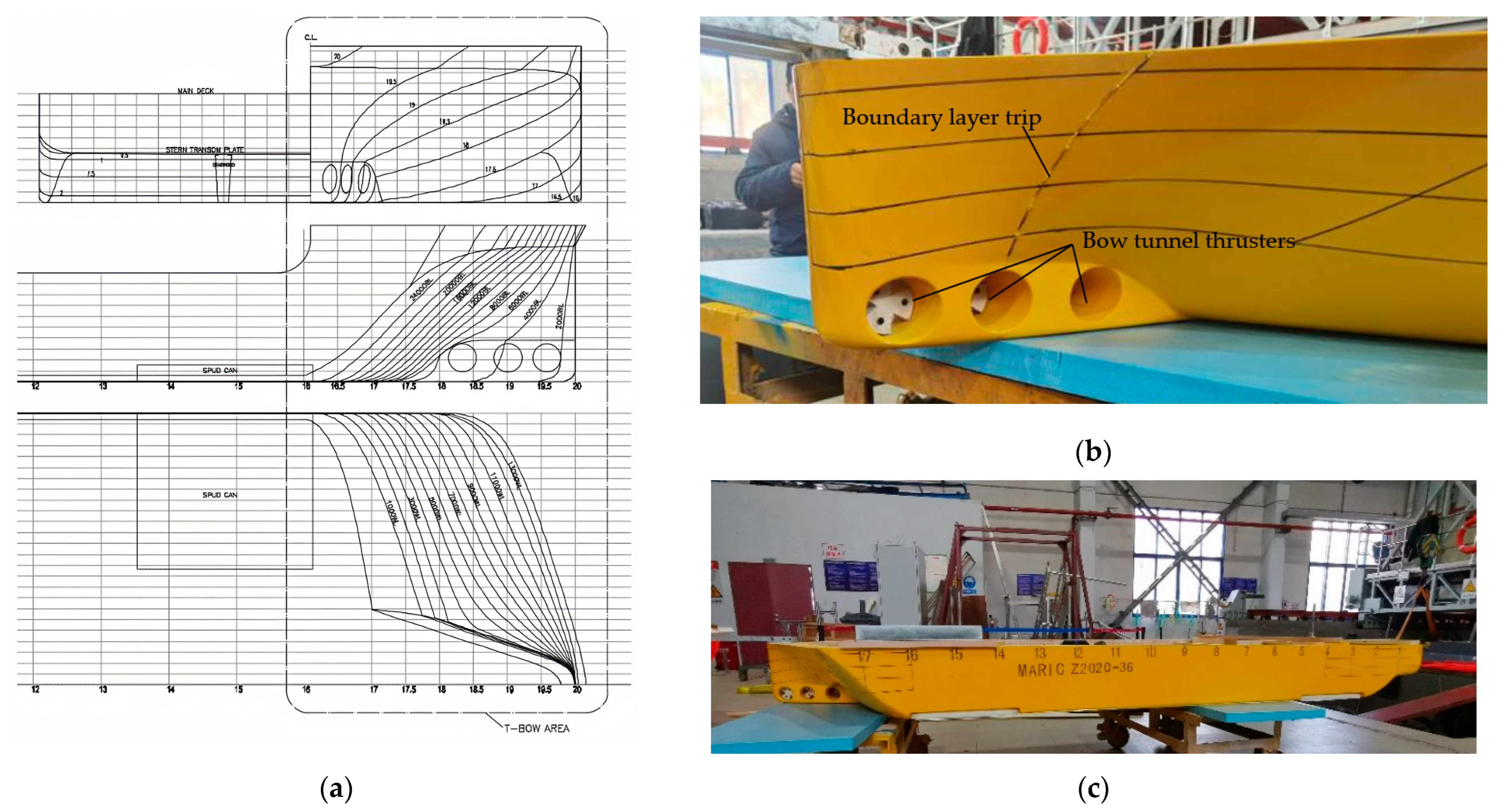
Thruster efficiency optimization: The new generation WTIVs are typically equipped with two or three sets of bow tunnel thrusters to maximize thruster efficiency while balancing the constraints of initial investment costs and requirements for DP-2 level dynamic positioning capabilities. Engineering principles dictate that the length of bow thruster tunnel structures should not exceed approximately six times the diameter of the propeller. However, design requirements for anti-overturning stability and a broad operational deck area often lead to vessel widths of 40–60 m. Traditional bows would result in excessively long rear bow thruster tunnels, which could compromise thruster efficiency. The T-BOW design effectively reduces the length of lateral thruster tunnels to enhance propeller efficiency.

Such design improvements are crucial for enhancing the propeller efficiency, dynamic positioning capacity, and anti-overturning stability under elevated conditions. The new generation WTIVs employing the T-BOW design are now widely used in China’s offshore wind construction fleet, as exemplified by vessels such as ‘ZHEN JIANG’, ‘TIE JIAN FENG DIAN 01’, ‘HY 78/79’, ‘BAI HE TAN’, and ‘LAN KUN 01’, etc., whose principal dimensions and key parameters are summarized in

Table 1. Main particulars and key parameters of the new generation WTIV with T-BOW in China.

Property	ZHEN JIANG	TIE JIAN FENG DIAN 01	HY 78/79	BAI HE TAN	LAN KUN 01
Length on water line, Lwl (m)	103.8	105	110.4	125	136
Breadth, B (m)	41	42	42	50	50
Depth, D (m)	8.2	8.5	8.5	10	10
Block coefficient, CB	0.822	0.824	0.834	0.801	0.816
Draft, T (m)	5.2	5.4	5.4	6.2	6
Speed, V (kn)	7	8	-	9	8
Azimuth thruster AFT	3 × 1800 kW	3 × 1800 kW	3 × 1800 kW	3 × 3000 kW	3 × 2600 kW
Bow tunnel thruster	3 × 750 kW	3 × 900 kW	3 × 900 kW	3 × 1500 kW	3 × 1600 kW
DP class	DP-1	DP-2	DP-1	DP-2	DP-2
Leg number & Type	4 × cylindrical shell type	4 × cylindrical shell type	4 × cylindrical shell type	4 × Triangular open truss type	4 × Triangular open truss type
Max. holding Capacity per Leg (t)	7000	7200	7200	13,500	14,000
Single Spudcan size (m2)	133	133	131	205	210
Deadwood number	2	2	2	2	2
Wind turbine installation capacity	8 MW	8 MW	10 MW	13 MW	15 MW

below.

From the above table, it can be seen that the new generation WTIVs have significant differences compared to conventional transport ships and auxiliary marine engineering vessels in terms of principal dimensions and hull form designs. The primary differences and the resulting resistance performance assessment and design challenges are outlined below:

(1)

Impact of Hull Form on Resistance: WTIVs generally feature a wide beam and a high block coefficient (C_B), leading to a bow design that exhibits a full and blunt form. This characteristic tends to induce blockage effects in the surrounding fluid flow, and the prominent shoulder region at the bow is prone to generating shoulder waves, which adversely affects wave-making resistance.

(2)

Bow and Stern Design Constraints: The necessity to accommodate spudcan structures results in rapid transitions in the hull lines at the bow and stern shoulder areas, characteristic of a full and blunt hull form. The limited space at the bow and stern necessitates sharp transitions towards the parallel midbody, which can lead to boundary layer separation and vortex formation. These phenomena adversely impact the viscous pressure resistance of the vessel.

(3)

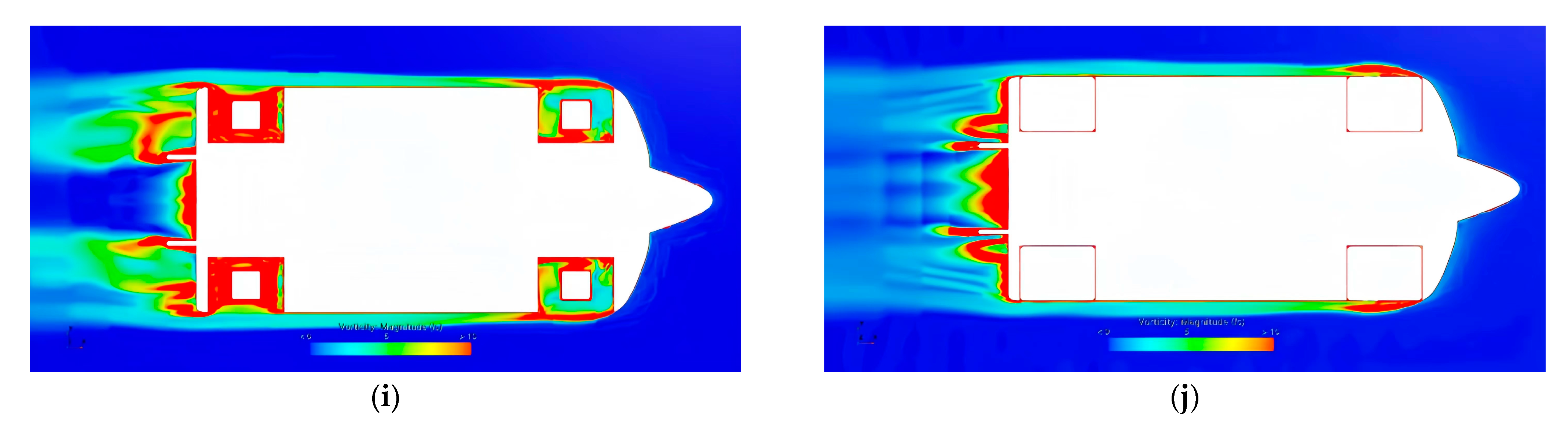
Additional Resistance Due to Appendages: WTIVs are equipped with various appendages, including skegs, sea chests, and bow tunnel thruster openings, as well as spudcan retraction well areas, which are vertical cavities that connect the deck to the hull bottom. For large WTIVs, the spudcan retraction well area can exceed 200 m², leading to significant “moonpool additional resistance” during navigation. Therefore, optimizing the spudcan structure design to align with the hull shell plate is crucial. Minimizing gaps and maintaining good flow continuity between the hull and spudcan structures is key to improving the vessel’s resistance performance.

Based on the comparative analysis above, resistance will be the primary challenge in WTIV design. Excellent resistance performance not only relates to the operational efficiency and fuel consumption cost of WTIV but also directly reflects the design of green ships. Achieving rapid and accurate resistance prediction during the hull form design process can greatly improve design efficiency and have significant engineering application value. Currently, ship resistance prediction methods mainly include ship model tests, CFD numerical prediction methods, and empirical formula estimation methods. Among them, ship model tests are time-consuming and costly, often used for the final verification of design results; CFD numerical prediction technology requires significant computational resources; empirical formula estimation is fast but difficult to control in terms of prediction accuracy.

The ship model test method mainly includes ship model manufacturing, towing tank tests, data processing (ship model to full-scale ship resistance extrapolation), etc. Uncertainty analysis is an important guarantee of the reliability of ship model test results (Kline [2]) and is a key focus of many scholars’ research. Guo et al. [3] investigated the resistance and flow field of the KVLCC2 ultra-large crude carrier with free heave and pitch, performing a comprehensive analysis of experimental uncertainty. Nikolov et al. [4] developed a linear mixed-effects model to quantify and combine uncertainties from various sources in high-speed planing boat resistance tests. Zhang Li et al. [5] analyzed uncertainties in ship model tests, addressing errors related to model construction, test installation, instrumentation, and measurement, and suggested methods to minimize test uncertainties by maintaining stable test conditions and enhancing towing system speed accuracy. Liu et al. [6] proposed an uncertainty analysis method considering ship–shore distance and water depth-induced uncertainties in ship–shore interaction contexts.

The CFD numerical simulation process includes steps such as establishing a three-dimensional hull form, setting up the computational domain, mesh generation, selecting turbulence models, and post-processing analysis. The ITTC [7] provides a process for ship CFD numerical simulation. CFD prediction accuracy is influenced by multiple factors, including modelling accuracy, computational domain size, mesh density, turbulence model selection, time step, and the number of iterations, making it a research hotspot in recent years. Wu et al. [8] conducted uncertainty analysis on the DTMB5415 standard model, identifying critical factors affecting numerical simulation results and quantifying various uncertainty components. Wang et al. [9] used the Latin Hypercube Sampling method to analyze the impact of first-layer boundary layer thickness, turbulence models, and mesh count on resistance calculations, offering optimization suggestions for CFD simulation settings. Islam et al. [10] performed uncertainty analysis on different hull forms using OpenFOAM, comparing two prevalent uncertainty analysis methods. Tong et al. [11] examined the effects of non-uniform flow and turbulence intensity on total resistance using CFD simulations and analyzed the uncertainties of the CFD results with uncertainty theory. Zhang et al. [12] and Chen et al. [13] referred to the ITTC’s recommended procedures to analyze the uncertainties of ship model resistance CFD numerical simulation results. The latter also analyzed the uncertainties of y+ values near the wall surface by changing the computational mesh density. Blanca et al. [14] reviewed the current state of turbulence model research in ship hydrodynamic applications, discussing the applicability and limitations of commonly used turbulence models and suggesting strategies for selecting turbulence modeling approaches in various ship simulation scenarios, including resistance prediction, flow simulation, self-propulsion, and cavitation analysis.

The empirical formula estimation method refers to the ship resistance prediction formulas developed using regression techniques based on existing ship data. It includes resistance estimation formulas based on graphical data (Bojovic [15], Radojcic et al. [16]) and estimation formulas such as Ayre, Lap-Keller, and Holtrop based on non-standard ship data. The empirical formula estimation method improves ship resistance prediction efficiency, allowing ship data to better serve hull form optimization design.

Presently, research on WTIV resistance is relatively sparse and limited to model testing and CFD numerical prediction methods. Xu [17] employed viscous turbulence theory and solved the Euler equations in an ideal fluid domain to obtain the viscous and wave-making resistance of WTIVs, validating the accuracy of numerical prediction methods through towing resistance model tests. Huang et al. [18] utilized free-form deformation and CFD methods to establish a UT Neural Network (UTNN) model between design variables and total resistance, optimizing the stern hull lines of WTIVs to achieve a design with excellent resistance characteristics. Zhuang et al. [19] used dual-mode theory in turbulence models and directly solved the Euler equations to analyze the viscous and wave-making resistance of WTIVs, verifying numerical prediction methods through model test results. Jing [20] measured calm water total resistance and main engine power at self-propulsion points under various speeds through scale model calm water resistance towing tests and self-propulsion tests. Combined with CFD numerical calculations, they determined the calm water total resistance of WTIVs and the proportion of wave-induced resistance in regular waves, comparing these with experimental values to calculate the propulsion power needed for the target ship. Kjær et al. [21] highlight the urgent need to optimize WTIVs for the global shift to renewable energy. They propose a novel CFD-based approach to accurately predict roll damping, offering valuable insights for WTIV operation and safety.

However, for WTIVs with relatively full and blunt bow and stern lines and special appendages such as legs, spudcans, skegs, and bow thruster tunnels, there is a lack of research on the proportion of resistance components, the impact of spudcan retraction wells on resistance, and quick estimation methods for resistance that meet practical engineering accuracy. Most ship model tests have not even simulated the structure of the spudcan well area.

This study integrates model tests, RANS-based CFD numerical prediction methods, and empirical formula estimation to comprehensively investigate WTIV resistance components, mechanisms, and prediction methods. First, an in-depth analysis of the resistance components and their generation mechanisms was conducted for “ZHEN JIANG”, China’s first self-propelled jack-up WTIV. Model experiments across various speeds revealed that residual resistance is the primary component, with viscous pressure resistance being the largest portion, followed by frictional and wave-making resistance. As speed increases, wave-making resistance becomes more significant at approximately 9.5 knots. Additionally, comparative model tests on calm water resistance were conducted for different spudcan retraction positions, revealing a from 20% to 30% resistance difference between the two schemes. CFD simulations indicated that this difference is mainly due to vortices generated in the cavity between the spudcan structure and the hull shell plate in the well area. Building on these analyses, optimization studies for the next-generation WTIV “BAI HE TAN” were performed by refining the ship’s main dimensions, bowlines, and spudcan well area design. This optimization reduced the residual resistance coefficient by from approximately 40% to 50%. Finally, using multivariate nonlinear least squares analysis, the resistance estimation methods based on the Holtrop method were modified, resulting in a resistance estimation approach suitable for WTIVs. The accuracy was verified using “LAN KUN 01”, a ship independent of the sample vessels, showing that the predicted speeds closely matched the final actual trail speeds, demonstrating that the revised resistance estimation formula meets practical engineering application accuracy requirements.

2. Methods for Resistance Prediction of WTIVs

In this paper, the calm water resistance data for two generations of self-propulsion wind turbine installation vessels (WTIV_O&N) based on the T-BOW hull form line plane were first obtained through model tests. Then, combining CFD numerical simulation predictions and the three-dimensional extrapolation method, an in-depth study and analysis were conducted on the resistance components, flow field, and vortex intensity distribution for WTIV_O under two spudcan retraction schemes—completely retracted above the baseline (Case_A) and spudcan edge flush with the baseline (Case_B)—at a series of speeds ranging from 3.0 to 12.0 knots. Finally, utilizing resistance sample data from multiple full-scale ships, the Holtrop empirical formula for different resistance components was modified through the Multivariate Nonlinear Least Squares Method to obtain a quantitative research method for WTIV resistance and rapidity.

2.1. Model Test Method

The model test method primarily involves the production of small-scale ship models according to similarity theory, conducting experiments in a test tank to obtain qualitative and quantitative data on the resistance of the target ship model. Many initial or excellent ships have acquired favorable resistance performance through model tests.

The main steps of the model test include model processing, test preparation, test implementation, data processing, and prediction of ship resistance conversion. In this paper, the towing tank used for the experiment measures 280 m in length, 10 m in width, and has a depth of 5 m. The main experimental instruments include the R63 resistance dynamometer, UB500 ultrasonic altimeter, and towing carriage, among others. The towing carriage is equipped with a computer real-time acquisition system. During the data measurement phase, the towing carriage maintains a constant speed, decelerating after sampling completion until stopped. The ship model is towed by the carriage, and the forces acting on the ship model at various speeds are recorded in real time by the computer. The ship model’s bow is equipped with a boundary layer trip to convert laminar flow into turbulent flow. During the resistance measurement phase, the ship model experiences free heave and pitch. Streamline testing employs the paint method, where painted ship models are towed at certain speeds in the tank by the towing carriage. By observing or measuring the paint traces left on the ship model, the desired streamline information is obtained.

Scaled model towing resistance tests were conducted with scale ratios of 27.333 and 35 for WTIV_O and WTIV_N, respectively. The water temperatures for the experiments were 9.5 °C and 15.5 °C. Both types of vessels were equipped with three sets of bow tunnel thrusters, four legs and spudcans, and two deadwoods at the stern, all adopting the T-BOW hull line plan as shown in Figure 1a. The primary parameters of the full-scale vessel and the model are compared and summarized in

Table 2. Ship particular represented by ship model.

Property	WTIV_O		WTIV_N
	Full-Scale Vessel	Test Model	Full-Scale Vessel	Test Model
Length overall, Loa (m)	103.8	3.7976	126	3.6
Length on water line, Lwl (m)	103.8	3.7976	125	3.5714
Breadth, B (m)	41	1.5	50	1.4286
Depth, D (m)	8.2	0.3	10	0.2857
Design draught, d (m)	5.2	0.1902	6.2	0.1771
Displacement, $∆$ (ton)	18,293	0.8932	32,530	0.7403

.

The ship models and deadwoods are constructed from wood with a smooth painted surface, while the spudcans are made of ABS material connected to the hull via stainless steel rods. The bilge keel is made of mild steel. The method of inducing turbulent flow involves placing a 1.15 mm diameter boundary layer trip wire at 1/20 L_wl from the perpendicular line of the ship model’s bow. The full-scale vessel’s hull line plan is depicted in Figure 2a, while the bow thruster structure and ship models are shown in Figure 2b and Figure 2c, respectively.

Through model tests, the total resistance $R_{tm}$ of the ship model can be obtained. The total calm water resistance data for the full-scale ship can then be calculated using the following formula:

$$R_{t(m/s)}=C_{t(m/s)}\times {\displaystyle \frac{1}{2}}\rho {V_{(m/s)}}^2{S}_{(m/s)}$$

(1)

$$C_{f(m/s)}=0.075/{(lg{R}_{n(m/s)}-2)}^2$$

(2)

$$C_{rm}=C_{tm}-C_{fm}$$

(3)

$$C_{ts}=C_{fs}+C_{rs}=C_{fs}+C_{rm}$$

(4)

where $R_n$ is the Reynolds number and $R_{ts}$ represents the total resistance of the full-scale ship. $C_{tm}$ and $C_{ts}$ are the total resistance coefficient of the ship model and the full-scale ship, respectively. $V_m$ and $V_s$ represent the speeds of the ship model and the full-scale ship, respectively. $S_m$ and $S_s$ are the hull wetted surface area for the ship model and the full-scale ship, respectively. Reynolds numbers for the ship model and the full-scale ship are indicated as $R_m$ and $R_s$, respectively. The residual resistance coefficients for the ship model and the full-scale ship are labeled $C_{rm}$ and $C_{rs}$, respectively. The frictional resistance coefficients for the ship model and the full-scale ship are denoted as $C_{fm}$ and $C_{fs}$, respectively.

2.2. Numerical Simulation Method

Computational Fluid Dynamics (CFD) techniques have found extensive application in elucidating the hydrodynamic performance of ships. This paper embarks on elucidating the theoretical underpinnings of the RANS methodology. It delineates the governing equations that encapsulate the interplay among diverse physical quantities within the flow field, delineates the requisite boundary conditions for solving the RANS equations, categorizes turbulence models, explicates discretization methodologies for the computational domain, elucidates the Volume of Fluid (VOF) approach for tracking free surface flows, and expounds upon boundary conditions. Rigorous convergence analyses are undertaken, scrutinizing grid generation dimensions and parameters, turbulence model selection within the framework of the Reynolds time-averaged approach, and optimal time step sizing. These analytical endeavors culminate in the development of a robust CFD numerical analysis method tailored specifically for WTIVs.

2.2.1. Governing Equations and Turbulence Model

The governing equations of the CFD method in this paper are the time-averaged continuity equation and RANS equations are as follows:

$${\displaystyle \frac{{\partial U}_i}{\partial x_i}}=0$$

(5)

$${\displaystyle \frac{\partial U_i}{\partial t}}+{\displaystyle \frac{\partial \left(U_i{U}_j\right)}{\partial x_j}}=g_i-{\displaystyle \frac{1}{\rho }} {\displaystyle \frac{\partial P}{\partial x_i}}+\nu {\displaystyle \frac{{\partial }^2{U}_i}{\partial x_j\partial x_j}}-{\displaystyle \frac{\partial \overline{u_i^{\prime }{u}_j^{\prime }}}{\partial x_j}}$$

(6)

Here,$u_i$ denotes the velocity of the fluid field; $U_i, U_j$ represent the components of the fluid average velocity; t denotes time; $x_i, x_j$ signify the coordinate components; $p$ denotes static pressure; $\nu$ stands for the fluid kinematic viscosity coefficient; $u_i^{\prime }, u_j^{\prime }$ depict the fluctuating components of velocity; $p^{\prime }$ symbolizes the fluctuating pressure; $g_i$ represents the force per unit mass acting on the fluid element; $\overline{u_i^{\prime }{u}_j^{\prime }}$ signifies the Reynolds stress.

Presently, in numerical simulations of viscous flow fields, commonly utilized two-equation turbulence models encompass k-ε series turbulence models (Standard k-ε, RNG k-ε, Realizable k-ε) and k-ω series turbulence models (Standard k-ω, SST k-ω) to close the RANS equations. Among these, the k-ε model proves efficacious for fully developed turbulence, i.e., high Reynolds number models, while the k-ω model boasts a broader application scope in mid-to-low Reynolds number problems. Especially the improved SST k-ω model simultaneously incorporates the advantages of both k-ε and k-ω models (Menter [22]), adding a cross-diffusion term and considering the influence of turbulent viscosity on turbulent shear stress. When simulating flow problems with large curved wall surfaces, it accurately predicts the logarithmic layer of pressure gradient flow and effectively resolves the sensitivity of the original model to the turbulence intensity of the inlet free stream (Xia [23]).

Given the intricacies of the T-BOW type WTIVs hull surface, this study undertakes a comprehensive evaluation of three closed turbulent models: the standard k-ε model, realizable k-ε model, and SST k-ω model, and employs the VOF model to trace and capture the dynamic free surface behavior.

2.2.2. CFD Modelling

The CFD modeling has been performed using the software STAR CCM+ (version 2022). This study employs a hull geometry model, as depicted in Figure 3a, accounting for the influence of bow tunnel thrusters and port and starboard sea chests on resistance. The numerical simulation utilizes a full model. The computational fluid domain is a rectangular prism, with the origin of coordinates defined at the intersection of the transom plate, the central longitudinal section, and the base plane. To ensure comprehensive capture of the free surface and interface wave generation within the domain, the bow is situated approximately 2 L_wl (waterline length) from the velocity inlet of the computational domain, and the ship’s sides are approximately 2 L_wl from the lateral boundary of the domain; the stern is approximately 5 L_wl from the outlet boundary of the domain. Ship boundary conditions are configured as shown in Figure 3b. Experimental tank temperatures and fluid densities are set based on relevant model test records. The top, bottom, inlet, and sides of the numerical tank are designated as symmetric boundary conditions, while the outlet employs a pressure outlet. A vertical damping method is implemented at the outlet to mitigate wave reflection effects on the results.

Due to fluid viscosity, the fluid adheres to the solid wall surfaces, with the fluid velocity at these points matching the velocity of the corresponding wall points. Boolean operations are applied to separate the hull from the towing tank, and non-slip grid conditions are enforced on the hull surface to maintain no-slip conditions at the wall. Dimensionless velocity $u^{+}$ and dimensionless length $y^{+}$ are introduced to describe the velocity distribution and thickness of the viscous sublayer at the wall. Through meticulous calculations and comparisons, it was determined that a first layer thickness of ∆y = 1 mm on the baseline grid yielded an average $y^{+}$ of approximately 30 on the ship model surface, meeting established criteria of 11.63~30 ≤ $y^{+}$ ≤ 200~500 (Yi et al. [24]).

In the numerical simulation, the ship moves at a constant velocity V in a straight line within the tank, utilizing a body-fixed coordinate system to study the problem as an infinite fluid flows past the ship. The partitioning of the fluid domain is illustrated in Figure 3b. Local grid refinement is applied to spudcans and their well structures, bow thruster tunnels, and appendages, such as skegs, with the corresponding three-dimensional fluid domain grid refinement depicted in Figure 3c,d.

2.3. Empirical Formula Estimation Method

The Holtrop estimation method was developed by the Dutch MARIN tank based on test data from 334 models and supported by extensive full-scale ship data (Holtrop [25]). The derived regression formulas are applicable for resistance estimation of various ship types. This approach utilizing a three-dimensional extrapolation not only considers wave-making resistance and viscous resistance but also accounts for additional resistance induced by modern ship features such as bulbous bows, stern flaps, and appendages. Currently, Holtrop’s method serves as a rapid resistance prediction tool in the preliminary design phase of ships, offering high computational accuracy (Julianto [26]).

However, with the ongoing increase in ship size and the continuous emergence of new ship types and operating conditions, engineers and researchers have focused on modifying the empirical formulas within the Holtrop method to enhance its accuracy and applicability. Nikolopoulos et al. [27] improved the Holtrop method by incorporating data from bulk carriers and tankers built between 2010 and 2016, along with model test data of the KVLCC2, enabling accurate resistance prediction for ships at low Froude numbers. Crudu et al. [28] refined the formula by adjusting the submerged depth of the bulbous bow and applied the modified formula to predict the resistance of a 37,000 dwt chemical tanker, achieving significantly improved prediction accuracy. Wang et al. [29] identified issues of low calculation accuracy and limited applicability in the empirical formulas for resistance estimation during the initial design phase, based on the database of newly constructed ship types. They revised several formulas within the Holtrop method using experimental data from the three main ship types (container ships, bulk carriers, and oil tankers), leading to a notable improvement in prediction accuracy.

Particularly for WTIVs with special appendages, such as legs and spudcans, which are typically full and blunt form vessels, the Holtrop method often yields considerable errors when used for resistance estimation of conventional ships. Therefore, this study bases its resistance estimation method on Holtrop’s approach, combined with the mechanisms of various resistance components and model test data. The Multivariate Nonlinear Least Squares Method is employed to correct the formulas for different resistance components, aiming to derive an empirical formula for WTIV resistance estimation that meets engineering calculation accuracy requirements.

The basic principle of the Multivariate Nonlinear Least Squares Method used in this study is as follows: given a fitting function$f\left(\theta ,x\right)$, observed input data$xdata$, and observed output data $ydata$, parameter vector $\theta$ that minimizes the sum of squared errors:

$$\underset{\theta }{\min }{‖f\left(\theta ,xdata\right)-ydata‖}_2^2=\underset{\theta }{\min }{\sum }_i{\left(F\left(x,{xdata}_i\right)-{ydata}_i\right)}^2$$

(7)

Here, $xdata$ includes basic dimensions and parameters of WTIVs necessary for resistance calculation, such as waterline length, beam, draft, and block coefficient, and so on, while $ydata$ represents the observed output data, such as the wetted surface area of the target ship, viscous pressure resistance, and wave-making resistance data from full-scale ship resistance measurements. Both $xdata$ and $ydata$ can be matrices or vectors, and $f\left(\theta ,xdata\right)$ is a matrix-valued or vector-valued function of the same size as $ydata$.

To obtain a more accurate and widely applicable empirical formula for the calm water resistance of WTIVs, this study utilizes full scale ship resistance data from a series of operational speeds for the vessels “ZHEN JIANG” (WTIV_O), “BAI HE TAN” (WTIV_N), and “TIE JIAN FENG DIAN 01” (WTIV_3) as correction and analysis sample data. This study focuses on refining the resistance calculation formula based on the Holtrop method. The accuracy of the revised formula was validated using the vessel “LAN KUN 01” (WTIV_4) as a case study. The key performance parameters of these vessels are detailed in Table 1.

3. Analysis of Calm Water Resistance of WTIV_O

3.1. Test Results of Calm Water Resistance

To delve into the influence of spudcan and its well structure design on WTIV resistance, model tests were conducted for two spudcan retraction schemes of WTIV_O: Case_A, where the spudcans are fully retracted above the baseline (Figure 4a), and Case_B, where the lower edges of the spudcans are aligned with the baseline (Figure 4b). The speed range considered was from 3.0 knots to 12.0 knots, with a test increment of 0.5 knots. A summary and comparison of calm water resistance test results are presented in

Table 3. The calm water resistance value of WTIV_ O under different speed.

Vs (kn)	Frm	Vm (m/s)	Case_A				Case_B
			Rtm	Ctm	Cfm	Crm	Rtm	Ctm	Cfm	Crm
			(N)	×103	×103	×103	(N)	×103	×103	×103
3.0	0.048	0.295	5.72	19.97	4.86	15.10	4.76	16.61	4.86	11.75
3.5	0.056	0.344	7.68	19.71	4.70	15.01	6.42	16.46	4.70	11.76
4.0	0.064	0.394	9.78	19.22	4.57	14.65	8.08	15.87	4.57	11.30
4.5	0.073	0.443	12.13	18.83	4.45	14.37	9.82	15.25	4.45	10.79
5.0	0.081	0.492	14.81	18.62	4.36	14.26	11.80	14.83	4.36	10.48
5.5	0.089	0.541	17.87	18.57	4.27	14.30	14.12	14.67	4.27	10.40
6.0	0.097	0.590	21.30	18.60	4.19	14.40	16.84	14.70	4.19	10.51
6.5	0.105	0.640	25.04	18.63	4.13	14.50	19.90	14.80	4.13	10.68
7.0	0.113	0.689	29.01	18.61	4.07	14.54	23.17	14.86	4.07	10.79
7.5	0.121	0.738	33.17	18.53	4.01	14.53	26.57	14.85	4.01	10.84
8.0	0.129	0.787	37.47	18.40	3.96	14.44	30.13	14.80	3.96	10.84
8.5	0.137	0.836	41.82	18.19	3.91	14.28	33.90	14.75	3.91	10.84
9.0	0.145	0.886	46.28	17.96	3.87	14.09	37.91	14.71	3.87	10.84
9.5	0.153	0.935	51.12	17.80	3.83	13.98	42.22	14.70	3.83	10.88
10.0	0.161	0.984	56.60	17.79	3.79	14.00	47.01	14.78	3.79	10.99
10.5	0.169	1.033	62.75	17.89	3.75	14.14	52.33	14.92	3.75	11.17
11.0	0.177	1.082	69.39	18.02	3.72	14.31	57.97	15.06	3.72	11.34
11.5	0.185	1.132	76.34	18.14	3.69	14.46	63.65	15.13	3.69	11.44
12.0	0.193	1.181	83.60	18.25	3.66	14.59	69.26	15.12	3.66	11.46

below.

In this study, resistance data from ship model tests, using a scaling ratio of 27.333, were extrapolated to obtain full-scale ship resistance data through the Equation (1) to Equation (4), where $F_{rm}$ denoting the Froude number for the ship model. It was established that total resistance exhibits a quadratic relationship with vessel speed. Notably, Case_A displayed a total calm water resistance from approximately 22% to 32% higher than that observed in Case_B. The dependency of full-scale ship total calm water resistance on speed is illustrated in Figure 5a. Furthermore, residual resistance constitutes the primary component of calm water resistance, accounting for approximately 90% and 86% of the total resistance in Case_A and Case_B, respectively. Coefficients of frictional and residual resistance are depicted in Figure 5b, where the residual resistance coefficient exhibits relative stability within the speed range of from 5 to 11 knots.

3.2. Analysis of Components of Calm Water Resistance

The calm water resistance derived from ship model tests for WTIVs consists of two main components: frictional resistance and residual resistance. The residual resistance encompasses viscous pressure resistance attributed to fluid viscosity and wave-making resistance. In order to delve deeper into the components of calm water resistance in WTIVs for targeted optimization and resistance reduction design, this study employs the three-dimensional extrapolation recommended as the standard at the 1978 ITTC conference, known as the (1 + k) method, to decompose residual resistance into its constituent parts. Due to space constraints, this paper focuses on the analysis of experimental results under the condition of spudcan retraction Case_B.

As shown in Table 3, within the Froude number range of from F_r = 0.1 to 0.2, the form factor (1 + k) can be determined using the method recommended by the 15th ITTC [30]. The equation used is as follows:

$$C_{tm}/C_{fm}=(1+k)+y{\displaystyle \frac{{F_r}^n}{C_{fm}}}, k=C_{pv}/C_f$$

(8)

where$C_{pv}$ is viscous pressure resistance, n ranges from 2 to 6 which is determined by ship type (for this study n = 2), and y and form factor (1 + k) are determined through least squares method based on C_tm and C_fm which are obtained from model tests. Linear regression analysis using the least squares method yields the form factor (1 + k) = 3.3729, as shown in Figure 6a.

The variations of each resistance component and their coefficients with respect to ship speed are ultimately derived and presented in Figure 6b,c. A comparative analysis of the data reveals that, except for the wave-making resistance coefficient, both frictional resistance and viscous pressure resistance coefficients decrease with increasing speed. Viscous pressure resistance emerges as the predominant component of calm water resistance, accounting for over 65% of the total, exceeding 80% at speeds below 6 knots. While wave-making resistance constitutes a relatively minor portion at lower speeds, significant wave making at the bow and water pile-up at the bow area become apparent from a speed of 7.0 knots onwards, as depicted in the experimental photographs in Figure 6d. From a speed of 9.5 knots, the wave-making resistance coefficient escalates rapidly with increasing speed, surpassing 20% at speeds exceeding 11 knots.

The observed inverse relationship between the coefficients of viscous pressure and wave-making resistance across the speed range of from 5 to 11 knots provides a clear explanation for the relatively stable residual resistance coefficient composed of these two factors. Frictional resistance contributes approximately 15% to the total calm water resistance, exhibiting minimal fluctuations with varying speeds.

3.3. Numerical Results of Calm Water Resistance

In order to delve more accurately into the mechanisms and patterns underlying the phenomena observed during experimental data analysis and testing, this study employs the WTIV_O experimental ship model as the focal point for computational analysis. Utilizing CFD numerical simulations are conducted to model two scenarios of spudcan retraction, with the objective of validating the accuracy of our numerical calculation methods, turbulence models, and parameter selection.

3.3.1. Precision and Convergence Analysis of the Numerical Method

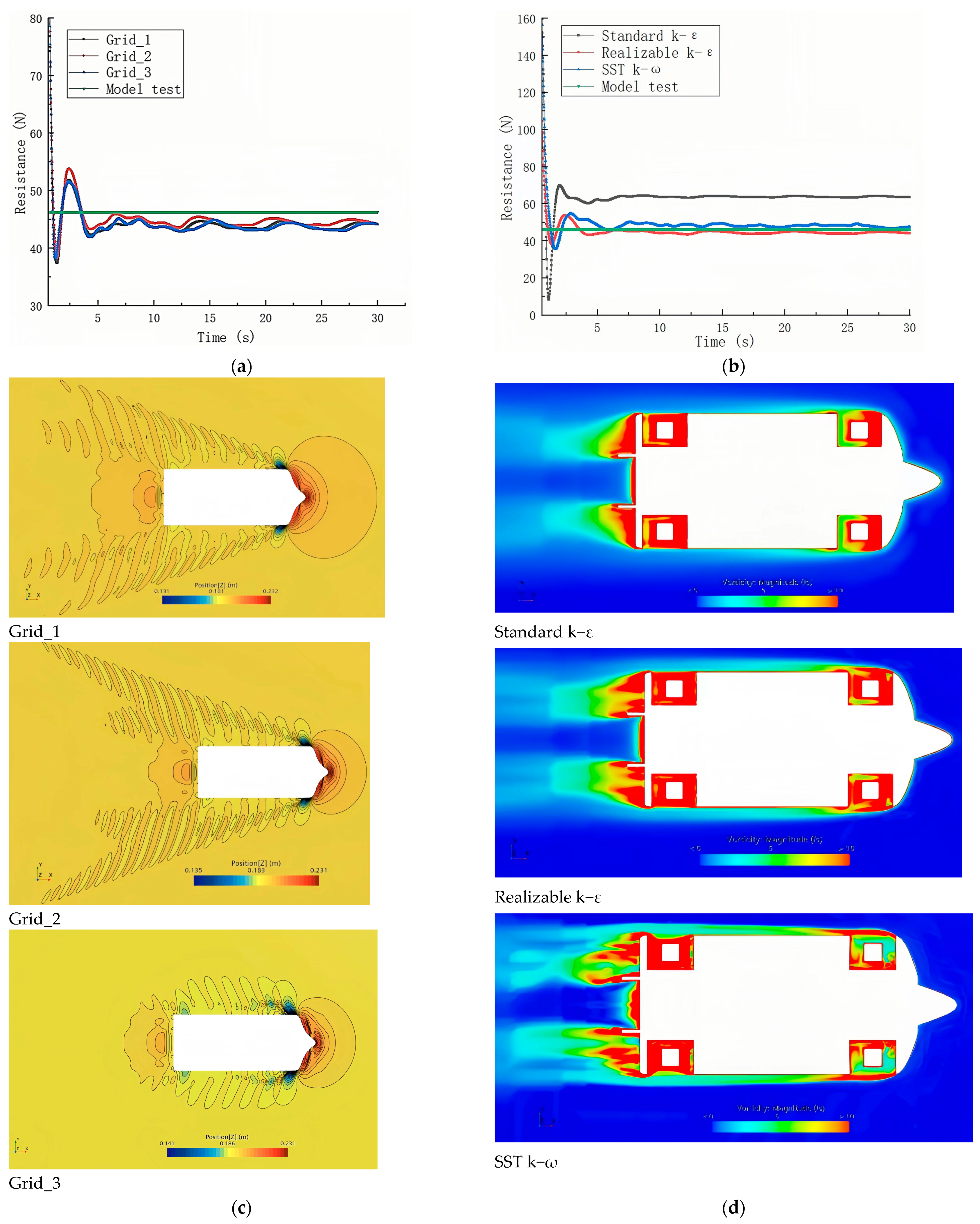
Drawing upon the WTIV model test data for ship resistance as a benchmark, this paper scrutinizes the influence of grid size, turbulence model, and time steps on the precision of numerical predictions of calm water resistance. It proposes an optimized parameter model for numerically predicting calm water resistance, tailored specifically for WTIV.

(1)

Mesh generation

To investigate the impact of grid size on the numerical calculation accuracy of resistance for WTIV, a time step of 0.020 s is set for simulating the static resistance of the ship model, employing the Realizable k-ε turbulence model. The computational fluid domain grid is segmented according to three fundamental size schemes outlined in

Table 4. Comparison of the resistance of different mesh gridding (F_r = 0.145).

Grid Scheme	Grid Size (m)	Grid Number (Million)	Numerical Value (N)	Experimental Value (N)	Error (%)	Computational Time (h)
Grid_1	0.076 (2.0% Lwl)	12.14	43.79	46.28	−5.38	3.8
Grid_2	0.106 (2.8% Lwl)	7.71	44.46	46.28	−3.94	2.4
Grid_3	0.152 (4.0% Lwl)	5.70	43.6	46.28	−5.79	1.9

, with a corresponding refinement ratio of $r_g=\sqrt{2}$. Figure 7a,c present the resulting time history curves of static resistance and the free surface wave pattern during static navigation of the ship model. Grid_1&2 effectively capture the Kelvin wave behind the ship and the stern wake. The convergence analysis results are succinctly summarized in Table 4.

By comparing computational analyses, it is evident that the precision of numerical predictions improves as the grid size of the fluid computational domain decreases. However, excessively small grid sizes can sometimes lead to the accumulation of Round-off Error during calculations, resulting not only in a significant increase in computational time but also occasionally distorting the calculation results (Hu [31], Deng [32]). Considering both the precision and efficiency of the computational results, this paper adopts the Grid_2 grid scheme to simulate the hydrodynamic resistance of the ship in calm water.

(2)

Turbulence Models

Using the aforementioned optimal grid scheme, Grid_2, with a time step of 0.020 s, we further analyze the influence of three turbulence models—Standard k-ε, Realizable k-ε, and SST k-ω—on the accuracy of calm water resistance calculations. The relevant calculation results are shown in

Table 5. Comparison of the resistance results using different turbulence models (F_r = 0.145).

Turbulence Models	Calculation Value (N)	Experimental Value (N)	Error (%)	Computational Time (h)
Standard k-ε	63.71	46.28	37.63	2.5
Realizable k-ε	44.46	46.28	−3.95	2.4
SST k-ω	48.04	46.28	3.78	2.7

. It is observed that there is little difference in both resistance calculation results and computational time among the selected turbulence models. However, the deviation between the resistance value calculated by Realizable k-ε and the experimental value exceeds 35%, whereas the deviations in the Realizable k-ε and SST k-ω calculated values from the experimental value are within 4%. The time history curves of calm water resistance calculated by the three turbulence models are illustrated in Figure 7b, and the free surface wave elevation and eddy strength distribution during static navigation of the ship model are shown in Figure 7c,d, where a stagnation point exists at the bow and vortices are generated at the stern, consistent with practical observations.

(3)

Selection of Time Step

Utilizing the aforementioned optimal grid scheme, Grid_2, and the Realizable k-ε turbulence model, we further analyze and compare the influence of three time steps—0.010 s, 0.020 s, and 0.030 s—on the calculation results of calm water resistance. The comparison between the calculated calm water resistance for each scenario and the model test value is shown in

Table 6. Comparison of the resistance results using different time steps (F_r = 0.145).

Time Step (s)	Calculation Value (N)	Experimental Value (N)	Error (%)	Computational Time (h)
0.010	44.53	46.28	−3.78	5.5
0.020	44.46	46.28	−3.93	2.3
0.030	44.4	46.28	−4.06	1.7

. The differences in calm water resistance results under the three time steps are minimal, but, as the time step decreases, the computational time increases rapidly. Therefore, it is recommended to use a time step of 0.020 s for calm water resistance simulations.

In summary, for the numerical prediction of calm water resistance for the T-BOW type WTIV, due to the presence of the leg and spudcan, deadwood, and bow tunnel thruster, the surface of the ship’s hull is complex, especially with pronounced curvature at the bow and stern, resulting in prominent diffraction issues. Compared to the Standard k-ε model, the Realizable k-ε and SST k-ω models better capture the flow separation phenomenon at regions of large wall curvature and simulate turbulent flow around the ship’s hull more accurately. Therefore, to ensure calculation accuracy and capture flow details, this paper employs the Realizable k-ε turbulence model, known for its strong predictive capability and robustness against inflow sensitivity, and the SST k-ω turbulence model, noted for its higher accuracy in predicting velocity profiles and frictional resistance.

3.3.2. Numerical Results of WTIV_O

Building upon the preceding analysis, this study employs the Realizable k-ε and SST k-ω turbulence models with a fundamental grid size of 2.8% L_wl and a time step of 0.020 s to conduct numerical predictions of WTIV’s calm water resistance across various trial speeds. A comparative analysis of computational results with experimental data is presented in

Table 7. Comparison of the resistance results of Case_A between model test and CFD.

Vs (kn)	Frm	Vm (m/s)	Rtm_EXP. (N)	SST k − ω		Realizable k − ε		Bare Hull
				Rt_CFD (N)	Error (%)	Rt_CFD (N)	Error (%)	Rt_CFD (N)	Difference with Case_A (%)
3.0	0.05	0.30	5.72	5.74	0.47	4.89	−14.47	3.92	−31.47
3.5	0.06	0.34	7.68	7.64	−0.57	6.59	−14.23	5.21	−32.16
4.0	0.06	0.39	9.78	9.93	1.44	8.62	−11.90	6.68	−31.70
4.5	0.07	0.44	12.13	12.46	2.76	10.88	−10.30	8.25	−31.99
5.0	0.08	0.49	14.81	15.30	3.35	13.41	−9.43	9.87	−33.36
5.5	0.09	0.54	17.87	18.12	1.40	16.06	−10.13	11.64	−34.86
6.0	0.10	0.59	21.30	21.43	0.63	19.11	−10.28	13.49	−36.67
6.5	0.11	0.64	25.04	24.89	−0.60	22.48	−10.22	15.63	−37.58
7.0	0.11	0.69	29.01	28.87	−0.49	26.1	−10.03	18.00	−37.95
7.5	0.12	0.74	33.17	33.21	0.13	29.97	−9.65	20.66	−37.71
8.0	0.13	0.79	37.47	37.81	0.91	34.4	−8.20	23.05	−38.48
8.5	0.14	0.84	41.82	43.01	2.84	39.06	−6.61	25.88	−38.12
9.0	0.15	0.89	46.28	48.04	3.80	44.46	−3.94	29.08	−37.17
9.5	0.15	0.94	51.12	53.89	5.42	49.99	−2.21	32.65	−36.13
10.0	0.16	0.98	56.60	59.47	5.07	55.81	−1.40	36.77	−35.04
10.5	0.17	1.03	62.75	66.27	5.60	62.45	−0.48	41.67	−33.59
11.0	0.18	1.08	69.39	73.06	5.29	69.35	−0.06	45.62	−34.26
11.5	0.19	1.13	76.34	80.96	6.06	77.06	0.95	51.18	−32.96
12.0	0.19	1.18	83.60	89.78	7.39	85.17	1.88	55.77	−33.29

.

The comparative analysis of numerical calculations and model experiments at different trial speeds reveals that, for F_r ≤ 0.15, the SST k-ω turbulence model yields higher accuracy, whereas, for F_r > 0.15, the Realizable k-ε calculations exhibit superior precision. This finding is consistent with previous studies conducted by researchers like Duan et al. [33] and Lin and He [34], who analyzed the impact of moonpools on drilling ship resistance and calculated numerical prediction accuracy for low-speed and high-speed vessels. Consequently, the numerical analysis method based on RANS, along with the selection of pertinent grid generation techniques, time steps, and turbulence models, meets the accuracy requirements for predicting WTIV’s calm water resistance.

3.3.3. Comparative Analysis of Streamline

At the designated speed of 7.0 knots for WTIV_O, the results of streamlines of the model test and CFD computation for the bow section are illustrated in Figure 8a,b. Due to rapid variations in the bow’s shape, a minor portion of water circumvents the outer bow towards the sides, while the majority flows downwards from the top to the bottom of the ship, leading to water accumulation and blockage at the bow. The streamline for the midship section, as depicted in Figure 8c,d, predominantly exhibits linearity along the ship’s longitudinal axis. Meanwhile, the streamline for the stern section, as shown in Figure 8e,f, displays a recirculation pattern owing to the stern lines’ sharp contraction. Additionally, given the lower pressure on the inner side of the deadwood compared to the outer side, a recirculation phenomenon occurs where water flows around the outer side of the deadwood towards the inner side after passing behind it.

3.4. Generation Mechanism of Resistance

Based on the experimental and CFD computational results, the generation mechanisms of the various resistance components of the WTIVs are conducted.

3.4.1. Viscous Pressure Resistance

As a primary component for the WTIV, the viscous pressure resistance is mainly determined by the aft body shape of the vessel. Figure 9a,b demonstrates that the sharp contraction of the stern lines leads to recirculation accompanied by severe boundary layer separation and extensive eddy formation, thereby increasing the viscous pressure resistance. Pressure distributions at the stern for speeds of 5 knots and 11 knots are shown in Figure 9c,d.

Regarding the bow section, due to the overly full and blunt bow, as illustrated in Figure 8b, there is a significant expansion of streamlines and a rapid increase in flow speed, especially at the bow shoulders, leading to a notable reduction in pressure. This increases the positive pressure gradient in the aft body, causing the flow to decelerate sharply, thereby also increasing the viscous pressure resistance. The pressure distribution at the bow is depicted in Figure 9e,f. According to the bow streamline test photographs and CFD calculation results shown in Figure 8a,b, it is evident that water flows diagonally from the bow sides into the bottom of the ship, facilitating boundary layer separation and the formation of bow eddies. The creation of these eddies forms a low-pressure area at the bottom of the bow, not only increasing the viscous pressure resistance but also contributing to the burying of the bow during navigation, thereby further increasing the resistance.

The flow streamline distribution and eddy intensity distribution in the spudcan retraction well area for two retraction schemes are detailed in Figure 9g,h. In Case_A, the presence of a moonpool-like cavity structure leads to a flow of water beneath the cavity, dragging the bottom water backward along with it. This reduces the pressure beneath the frontal wall of the spudcan enclosure, with upper water replenishing from above, lowering the free surface. The presence of a vertical rear wall in the enclosure creates a blocking effect, causing the water to collide against it at a high velocity and forcing it upward, raising the free surface near the rear wall. The formation of eddies in the upper part of the cavity as the water replenishes forward contributes to water being transported towards the stern, reducing the pressure at the stern and further increasing the viscous pressure resistance. Thus, Case_A exhibits a more pronounced ‘moonpool additional resistance effect’, with significantly higher eddy strength than Case_B, resulting in increased residual resistance. Furthermore, for such full and blunt vessels, especially those with large forebodies, external bow eddies are typically generated at the bow and internal stern eddies at the stern, as shown in Figure 9i,j.

3.4.2. Wave-Making Resistance

Photographs of the traveling waves recorded during trials and comparative wave pattern charts based on CFD calculations, at speeds of 5 knots, 7 knots, and 10 knots, are shown in Figure 10a–c. The comparison reveals that the CFD numerical prediction results are in good agreement with experimental observations, displaying the following characteristics:

(1)

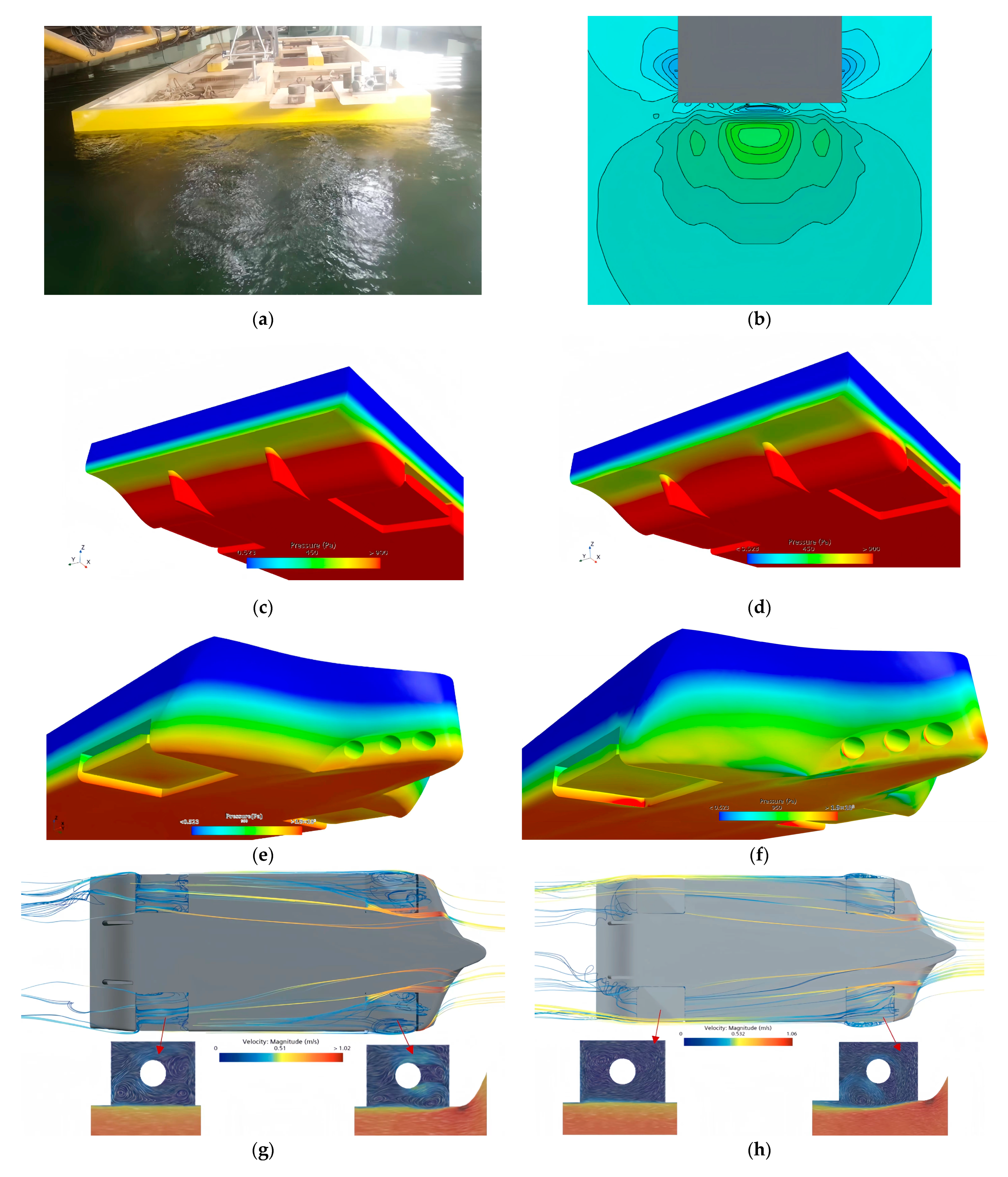
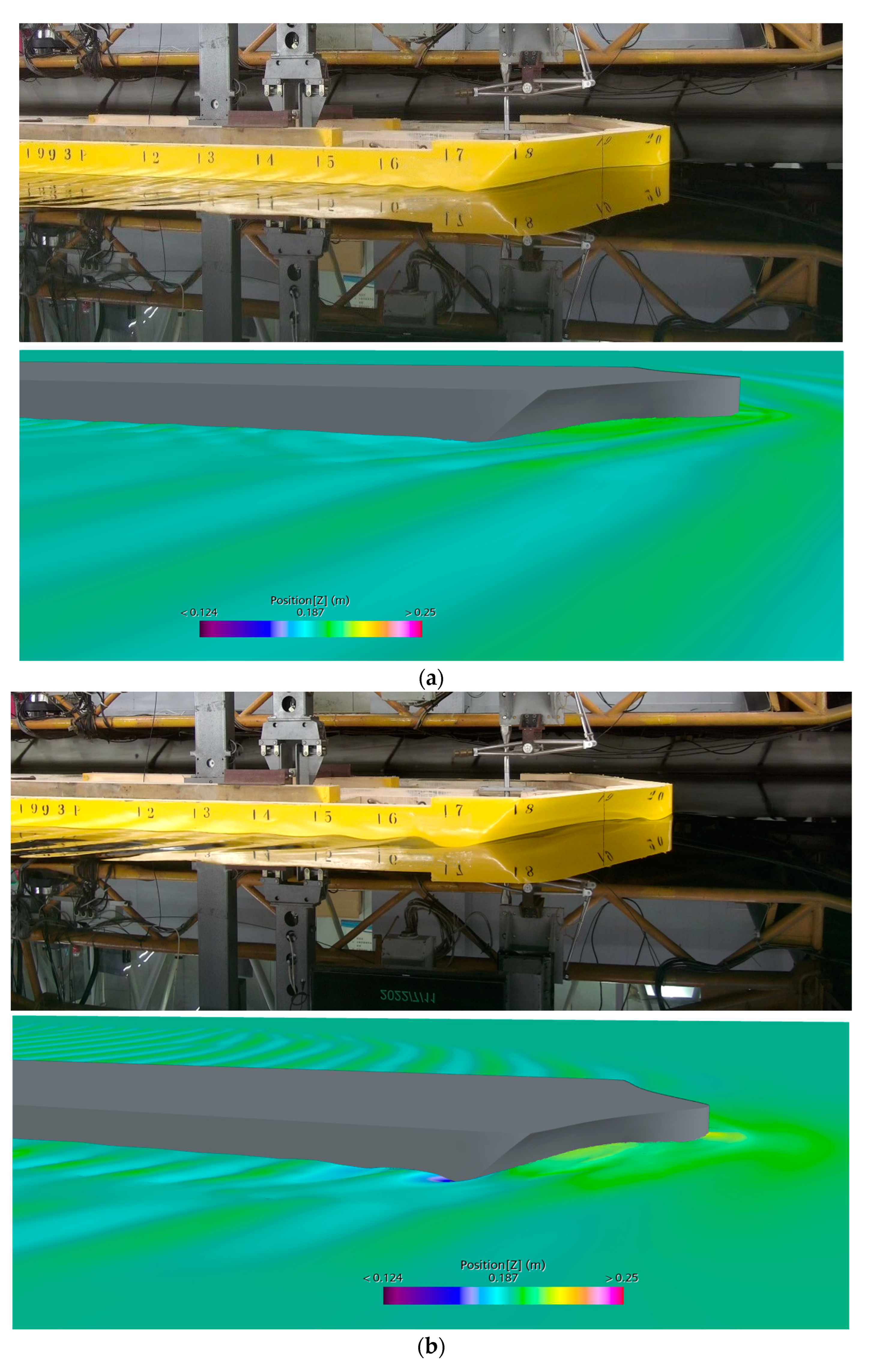
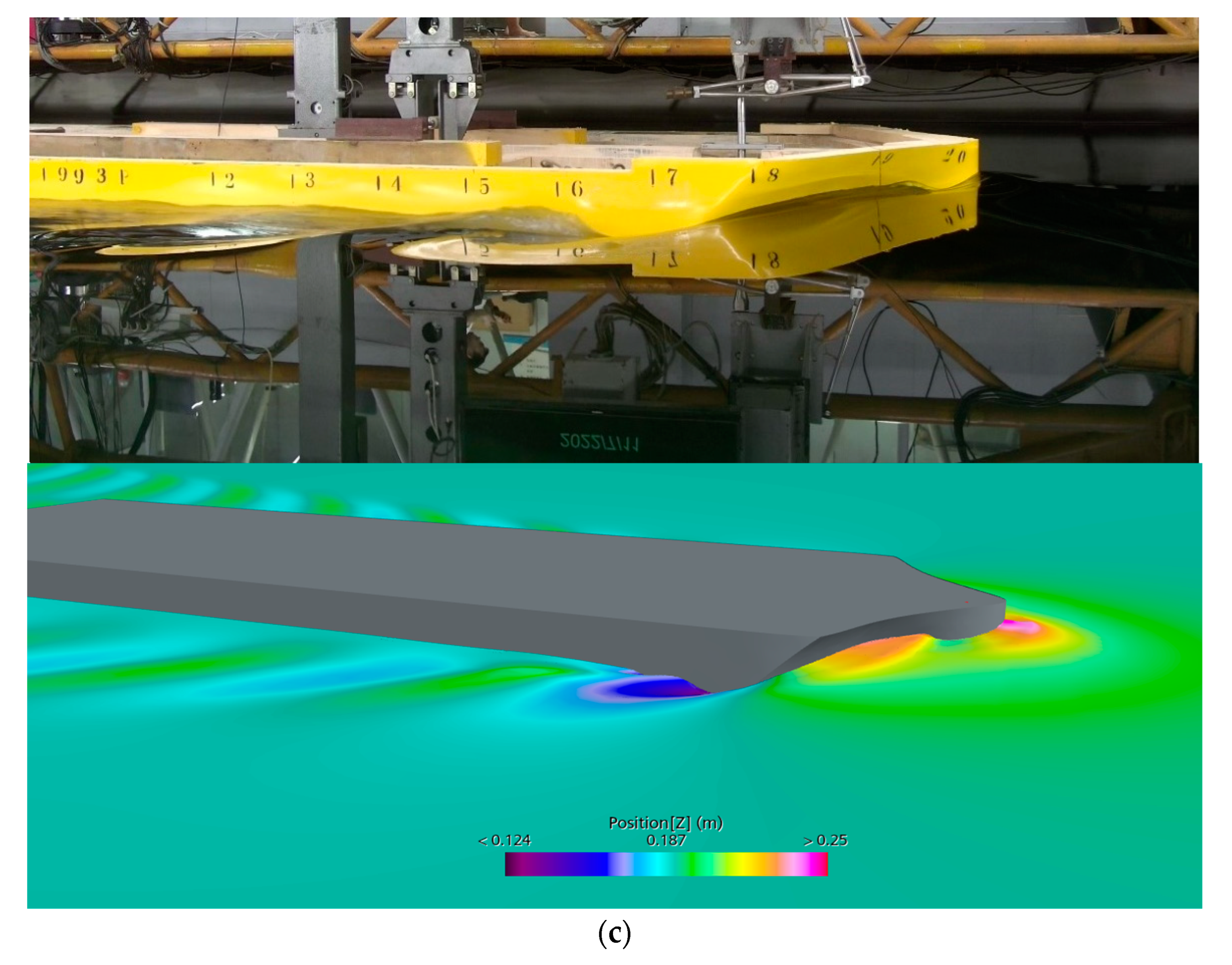
The generation of ship waves by WTIV is primarily due to changes in fluid pressure around the ship while navigating on the water surface, especially as the speed increases, creating a maximum pressure area at the bow shoulders, where the wave-making effect is strongest, as depicted in Figure 10c. Following this are the stern shoulders, where the line type changes abruptly, also producing noticeable stern shoulder waves. Such shoulder waves not only increase the ship’s wave-making resistance but may also cause adverse wave interference.

(2)

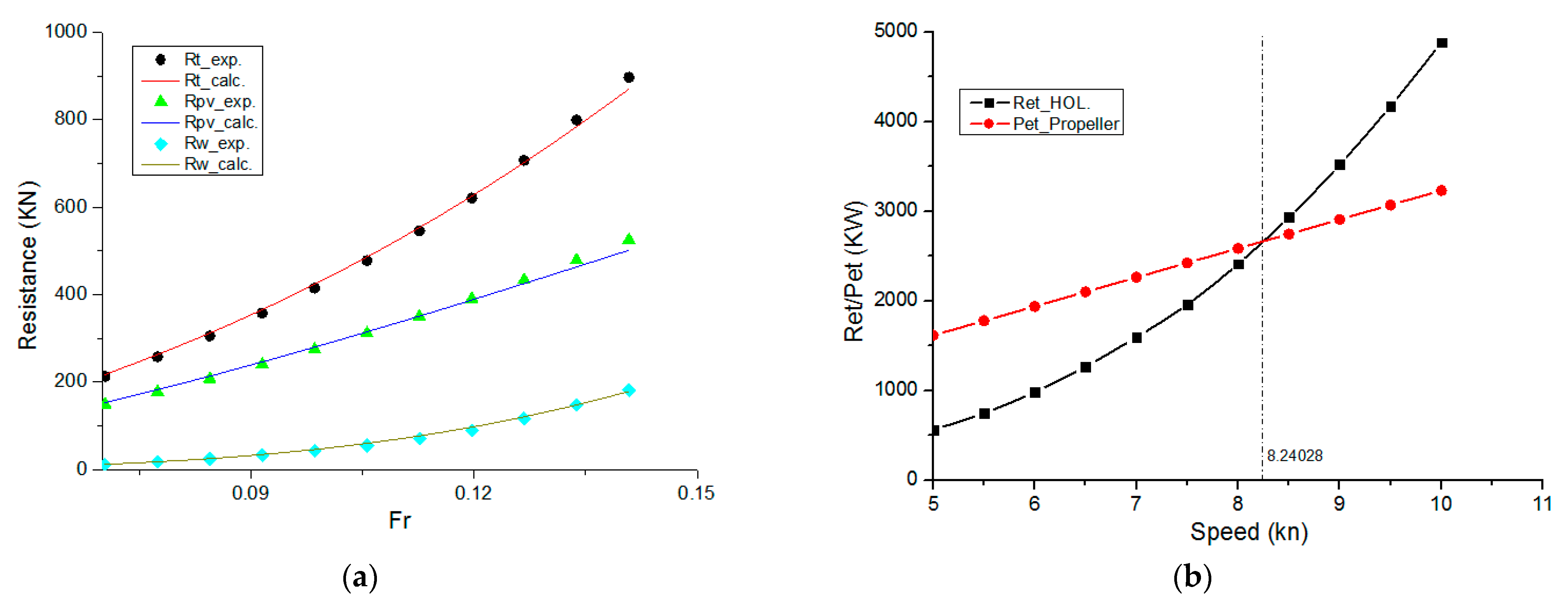
Analysis shows that the wave-making resistance of the WTIV is related to speed by a power function, with the proportion of wave-making resistance components increasing rapidly when the speed exceeds 9.5 knots.

3.4.3. Appendage Resistance

Comparative analysis of data from Table 7 reveals a significant increase in the proportion of appendage resistance components for WTIV compared to conventional transport vessels. In addition to conventional appendages, such as sea chests and bow tunnel thrusters, WTIV incorporates four spudcan retraction well areas, particularly impacting Case_A, where the influence exceeds 30%. The primary components of appendage resistance are viscous pressure resistance and frictional resistance. During the design process, careful attention is required to the influence of appendage shapes, especially at the spudcan retraction well areas. Efforts should be made to minimize the gap between the ship’s side and bottom outer plates and the spudcan structure, aiming to reduce the formation of vortices generated by appendages and consequently decrease viscous pressure resistance.

4. Optimization for Resistance Reduction of Next-Generation WTIV

4.1. Optimization Strategy

According to the analyses of resistance for WTIV_O, when conducting resistance reduction optimization of WTIVs, the following aspects should be prioritized:

(1)

Bow structure, particularly the effective transition of line types in the spudcan retraction well area, with the aim to minimize excessive curvature and disturbances to the wave system at the bow shoulders.

(2)

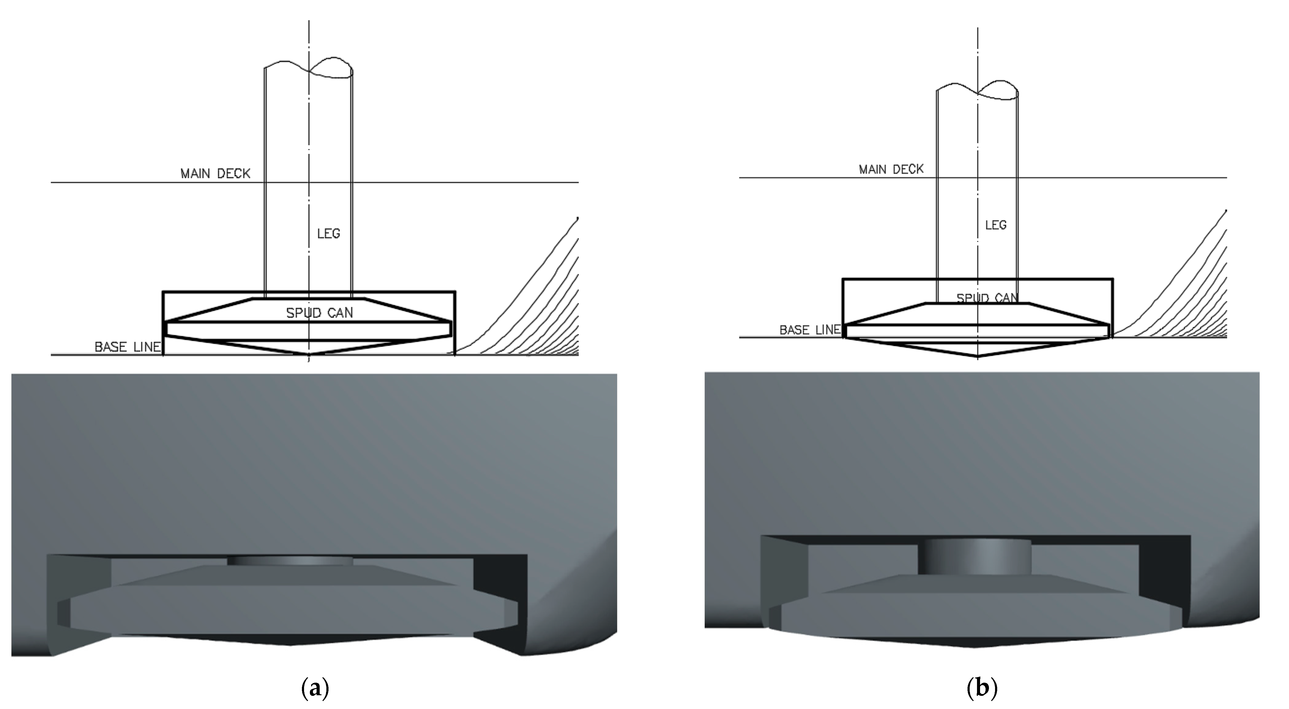
Matching design between the spudcan structure and the ship’s bottom and side outer shells in the retraction well area to mitigate the “moonpool additional resistance effect” in the relevant region.

(3)

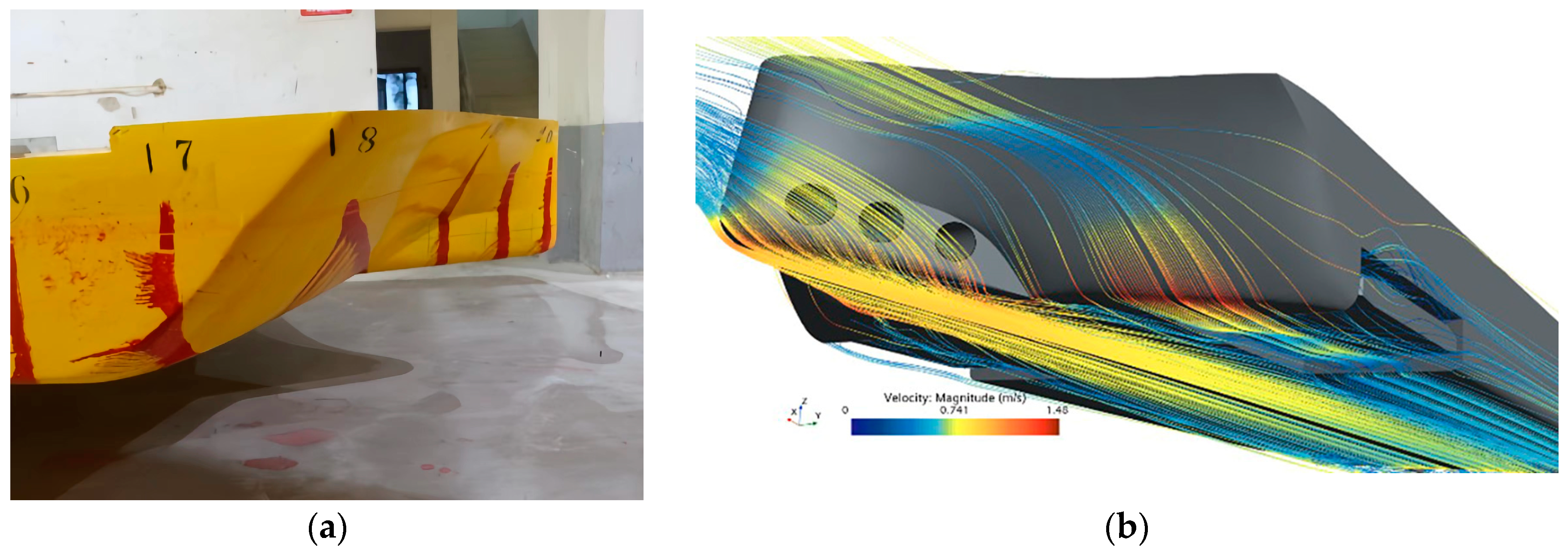
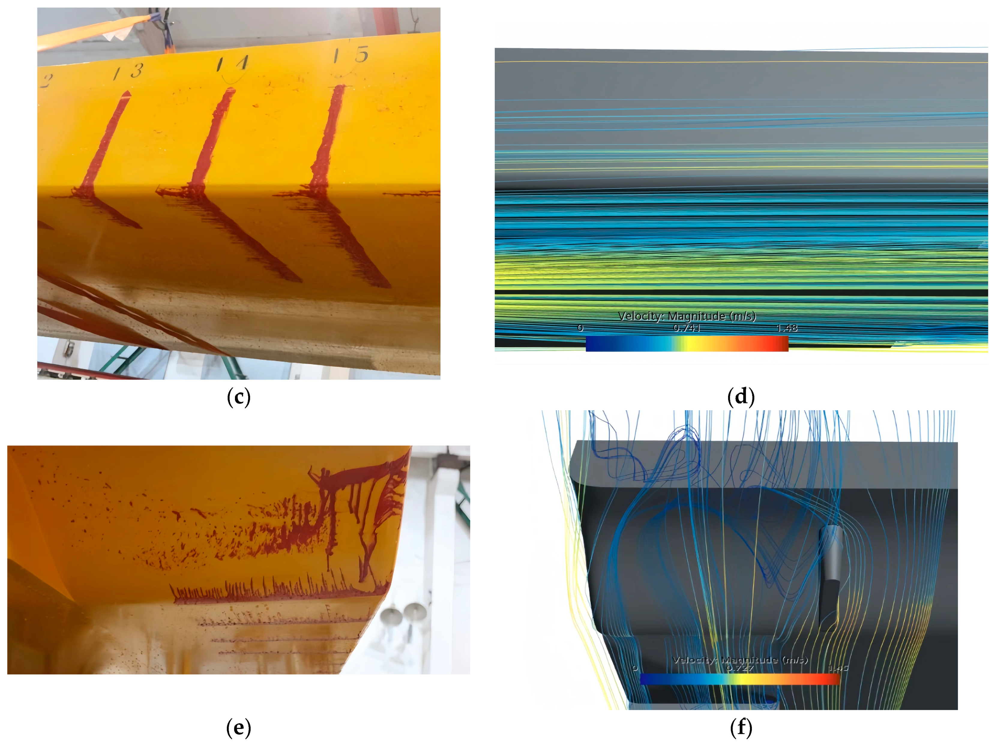
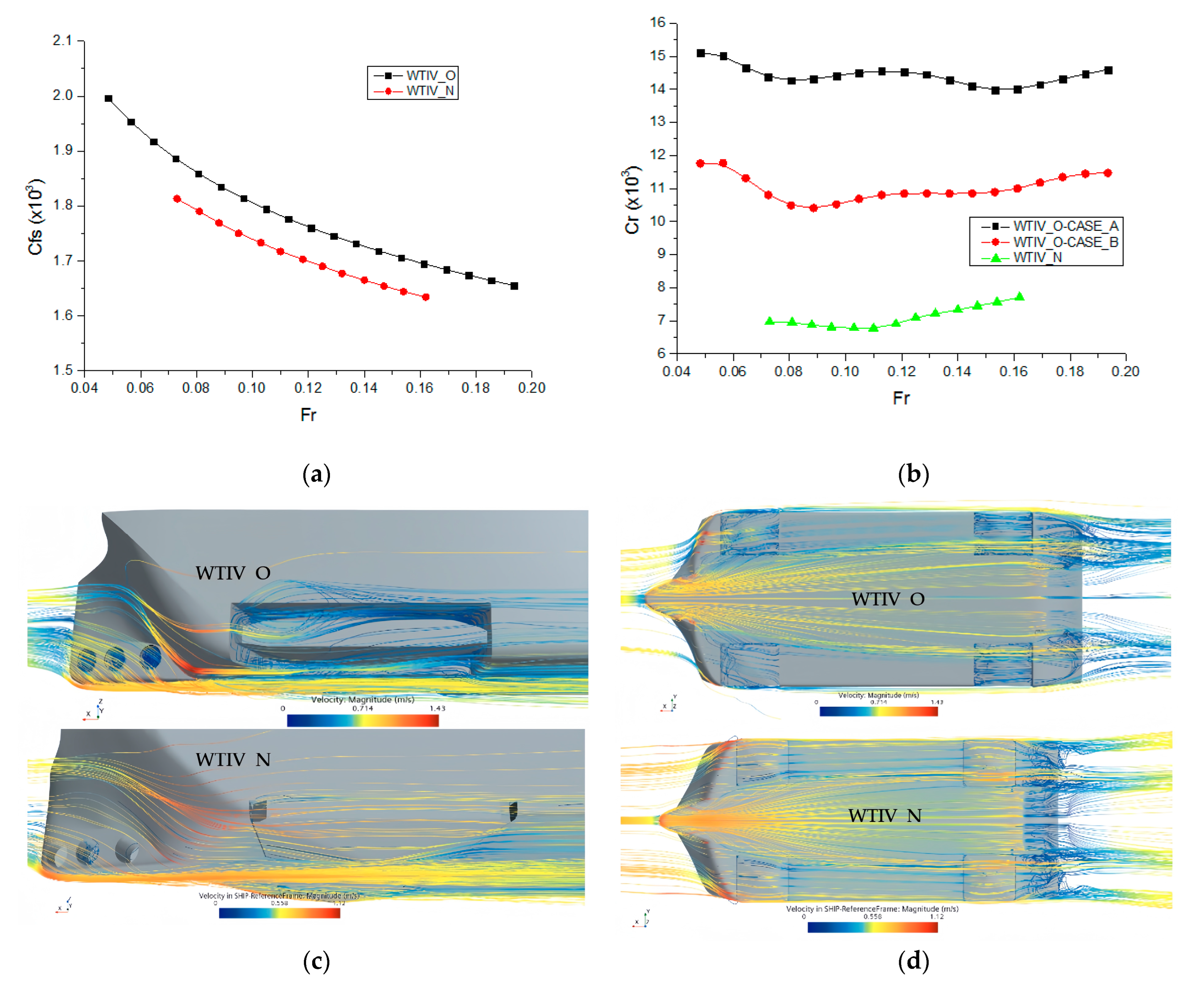
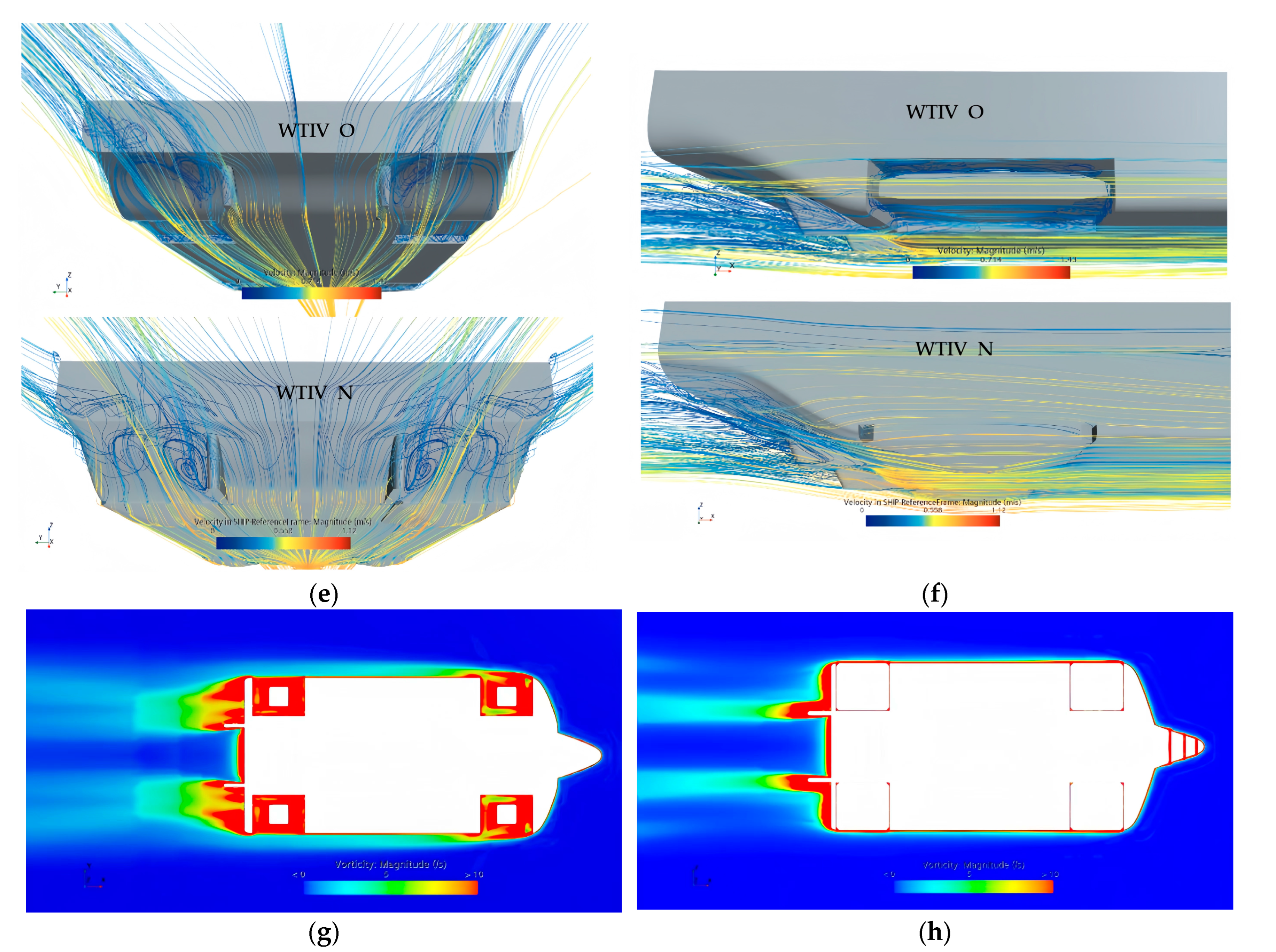
Considering the balance between displacement and weight distribution, the focus should be on the aft body’s flow design to ensure smoother fluid motion, more uniform pressure distribution, and reduced formation of stern vortices and energy loss, consequently lowering viscous pressure resistance.

In this study, model tests are conducted to measure the optimized resistance of WTIV_N, evaluating the effectiveness of the optimizations. Key optimization measures include aligning the edge of the spudcan with the baseline in Case_B and effectively sealing the side outer plates along the spudcan contour in the retraction well area, as depicted in Figure 11a. These measures not only reduce structural stress concentrations in corner regions but also diminish the “moonpool additional resistance” in the area. Photographs of the optimized spudcan and its retraction well are presented in Figure 11b, while the bow region profile optimization schemes are illustrated in Figure 11c,d.

4.2. Optimization Results

The summarized calm water resistance data from model tests of the WTIV_N are presented in

Table 8. The calm water resistance data of WTIV_ N value under different velocities.

Vs (kn)	Fr	Rtm (N)	Ctm × 103	Cfm × 103	Cr × 103	Cfs × 103	Cts × 103	Rts (kN)
5	0.073	6.44	11.336	4.375	6.961	1.813	8.774	236.46
5.5	0.081	7.72	11.232	4.289	6.943	1.790	8.732	284.76
6	0.088	9.06	11.079	4.213	6.866	1.769	8.635	335.13
6.5	0.095	10.50	10.943	4.144	6.799	1.750	8.549	389.38
7	0.103	12.08	10.855	4.082	6.773	1.733	8.506	449.32
7.5	0.110	13.79	10.794	4.026	6.769	1.717	8.486	514.60
8	0.118	15.80	10.871	3.974	6.897	1.703	8.600	593.34
8.5	0.125	18.08	11.015	3.926	7.088	1.690	8.778	683.69
9	0.132	20.40	11.091	3.882	7.209	1.677	8.886	775.91
9.5	0.140	22.89	11.166	3.841	7.325	1.665	8.990	874.68
10	0.147	25.54	11.246	3.802	7.444	1.654	9.098	980.84
10.5	0.154	28.36	11.326	3.766	7.559	1.644	9.203	1093.86
11	0.162	31.44	11.439	3.733	7.706	1.634	9.340	1218.35

. A comparison of the relevant data reveals that, under Case_B where the spudcan edge aligns with the bottom shell plate, the increase in vessel length and local profile optimization significantly reduces viscous pressure resistance. Consequently, the residual resistance coefficients at various cruising speeds exhibit a considerable decrease compared to WTIV_O, with reductions of from approximately 45% to 55% for Case_A and from 30% to 40% for Case_B. The comparative coefficients of frictional resistance and residual resistance for both vessels are depicted in Figure 12a and Figure 12b, respectively.

To more visually compare the streamline and eddy intensity before and after optimization, this paper presents streamlines at a cruising speed of 9 knots in the bow-stern and spudcan retraction well areas, as shown in Figure 12c–f. The optimization clearly improves the flow field, particularly reducing vortices in the retraction well area, as demonstrated by the overall vessel eddy intensity distribution in Figure 12g,h.

5. Empirical Formulas of WTIV Resistance Estimation Based on Holtrop Method

This study extends the Holtrop resistance estimation method by integrating model test data and numerical results. Utilizing the Multivariate Nonlinear Least Squares Method, the formula for the total resistance of the actual WTIV ship is presented as follows:

$$R_{\mathrm{T}}=R_{\mathrm{t}\mathrm{c}\mathrm{l}\mathrm{a}\mathrm{m}}+∆R_F+R_{aa}$$

(9)

Here, $R_{\mathrm{t}\mathrm{c}\mathrm{l}\mathrm{a}\mathrm{m}}$ represents the calm water resistance of the vessel, while $∆R_F$ and $R_{aa}$ account for resistance adjustments due to hull surface roughness and air resistance, respectively. The coefficients $∆C_f$ and the air resistance coefficient are computed using the 15th ITTC recommendations. The primary focus of this study is the calm water resistance of the WTIV, which is computed as follows:

$$R_{\mathrm{t}\mathrm{c}\mathrm{l}\mathrm{a}\mathrm{m}}=R_{\mathrm{F}}+R_w+R_{pv}$$

(10)

where $R_{\mathrm{F}}$ denotes the frictional resistance, $R_w$ stands for the wave-making resistance, and $R_{pv}$ represents the viscous pressure resistance.

In this study, the sample data of three full-scale ship resistance data are provided in

Table 9. Sample data of resistance components.

VS (kn)	RTPV_EXP (kN)			Rw_EXP (kN)			Rtclam_EXP (kN)
	WTIV_O	WTIV_N	WTIV_3	WTIV_O	WTIV_N	WTIV_3	WTIV_O	WTIV_N	WTIV_3
3	76.46	-	-	1.45	-	-	91.13	-	-
3.5	100.61	-	-	5.55	-	-	123.77	-	-
4	127.67	-	-	5.51	-	-	155.76	-	-
4.5	157.58	-	-	3.39	-	-	189.09	-	-
5	190.28	172.37	197.89	2.66	15.23	6.52	227.15	236.46	239.77
5.5	225.71	204.46	234.74	6.07	21.95	13.36	272.64	284.76	290.34
6	263.83	238.98	271.75	14.85	27.50	25.25	326.74	335.13	346.68
6.5	304.61	275.91	307.65	27.64	33.75	44.22	388.04	389.38	409.56
7	348.00	315.20	351.48	41.62	42.57	66.59	453.69	449.32	484.31
7.5	393.97	356.83	397.91	55.12	53.63	88.19	521.97	514.60	561.45
8	442.50	400.77	446.92	68.60	75.07	109.76	593.31	593.34	641.68
8.5	493.55	447.00	498.49	83.33	105.11	133.34	668.95	683.69	727.01
9	547.10	495.49	552.57	99.86	133.98	164.77	749.40	775.91	823.26
9.5	603.13	546.22	609.16	120.13	166.45	204.23	836.60	874.68	930.57
10	661.62	599.17	661.62	147.91	203.33	248.50	934.27	980.84	1039.08
10.5	722.54	654.33	715.31	184.43	244.14	302.47	1043.62	1093.86	1159.07
11	785.87	711.67	770.15	224.84	293.52	370.98	1159.78	1218.35	1295.26
11.5	851.60	-	832.86	262.97	-	447.05	1276.56	-	1447.40
12	919.71	-	892.12	296.17	-	533.10	1391.30	-	1606.59

.

5.1. Empirical Formulas of Frictional Resistance Estimation

The frictional resistance of the full-scale WTIV ship is divided into bare hull frictional resistance $R_{\mathrm{F}\_hull}$ and appendage frictional resistance $R_{\mathrm{F}\_APP}$, calculated as follows:

$$R_{\mathrm{F}}{=R}_{\mathrm{F}\_hull}+R_{\mathrm{F}\_APP}={\displaystyle \frac{1}{2}}\rho V^2{S}_{hull}{C}_f+{\displaystyle \frac{1}{2}}\rho V^2{S}_{APP}{C}_f$$

(11)

Here, $\rho$ represents the density of seawater, $V$ is the vessel’s speed, m/s, $S_{hull}$ is the wetted surface area of the bare hull, m², $S_{APP}$ is the wetted surface area of appendages such as legs and spudcans, and $C_f$ is the friction resistance coefficient calculated using the ITTC-1957 formula.

Estimating the bare hull wetted surface area $S_{hull}$ accurately for WTIVs poses a significant challenge due to the complex bow and stern lines. While the wetted surface area of appendages $S_{APP}$ can be precisely computed using simple geometric area formulas, the bare hull wetted surface area $S_{hull}$ requires a formula, the calculation formula is outlined as follows:

$$S_{hull}=L_{wl}\left(2T+B\right)\sqrt{C_M}\left({\mathrm{X}}_1+{\mathrm{X}}_2{C}_B+{\mathrm{X}}_3{C}_M+{\mathrm{X}}_{4}B/T+{\mathrm{X}}_5{C}_W\right)$$

(12)

Here, $T$ denotes the design draft, B stands for the breadth, $C_M$ denotes the midship section coefficient, $C_B$ stands for block coefficient, $C_w$ is the water-plane coefficient, and ${\mathrm{X}}_{1~5}$ are correction coefficients.

After Multivariate Nonlinear Least Squares analysis based on the full-scale wetted surface areas given in Table 9, the correction coefficients for the aforementioned formulas were determined. The corrected formula applicable to WTIVs with T-BOW for the bare hull wetted surface area $S_{hull}$ calculation is articulated as follows:

$$S_{hull}=L_{wl}\left(2T+B\right)\sqrt{C_M}\left(-2.0405+0.4459C_B+2.61C_M+0.0014B/T-0.0417C_W\right)$$

(13)

Using the formulas, the estimated wetted surface areas for a series of WTIVs have been compared with the actual numerical results. These comparisons are summarized in

Table 10. Comparative analysis of estimated and full-scale wetted surface areas for WTIV bare hulls.

Parameters	ZHAN JIANG WTIV_O	BAI HE TAN WTIV_N	TIE JIAN 01 WTIV_3	LAN KUN 01 WTIV_4	HY 78/79 WTIV_5	HUA XIANG LONG WTIV_6
L (m)	103.8	125	105	136	110.4	130
B (m)	41	50	42	50	42	42
T (m)	5.2	6.2	5.4	6	5.4	6
CM	0.9985	0.9995	0.9994	0.9995	0.999	0.9983
CB	0.818	0.801	0.824	0.816	0.834	0.814
CW	0.925	0.801	0.923	0.816	0.928	0.855
Target value (m2)	4832.7	7039.2	5025	7662.2	5305.6	6322.9
Estimated value (m2)	4808.84	7037.35	5026.65	7661.84	5302.79	6322.26
Error (%)	−0.496%	−0.026%	0.033%	−0.005%	−0.053%	−0.010%

. The comparison demonstrates that the estimated bare hull wetted surface area of the WTIV closely aligns with actual numerical results, with an estimation error controlled within ±0.5%.

5.2. Empirical Formulas of Viscous Pressure Resistance Estimation

The practical viscous pressure resistance of WTIVs consists of the hull viscous pressure resistance $R_{pv\_hull}$, the appendage viscous pressure resistance $R_{pv\_APP}$, and the pressure resistance of the immersed stern transom plate $R_{TR}$. It is calculated as follows:

$$R_{pv}=R_{pv\_hull}+R_{pv\_APP}+{\alpha R}_{TR}$$

(14)

$$R_{pv\_hull}=(1+k_1)R_{F\_hull}-R_{F\_hull}$$

(15)

$$R_{pv\_APP}={(1+k_2)}_{eq}{R}_{F\_APP}-R_{F\_APP}$$

(16)

$$R_{TR}=0.5\rho v^2{A}_T{C}_6$$

(17)

Here, $(1+k_1)$ and ${(1+k_2)}_{eq}$ are form factors relating to the relationship between hull and appendage viscous pressure resistance and their respective frictional resistances. $C_6$ is a coefficient associated with the Froude number of the immersed stern transom plate, and $\alpha$ is a correction coefficient. The calculation formulas are given as follows:

$$(1+k_1)=C_{13}\left[0.93+C_{12}{\left({\displaystyle \frac{B}{L_R}}\right)}^{{\beta }_4}{\left(0.95-C_p\right)}^{{\beta }_5}{\left(1-C_p+0.0225l_{CB}\right)}^{{\beta }_6}\right]$$

(18)

$${(1+k_2)}_{eq}={\sum }_{i=1}^n\left(1+k_2\right)S_{AP{P}_i}/{\sum }_{i=1}^n{S}_{AP{P}_i}$$

(19)

$$C_6=\left\{\begin{array}{c}0.2\left(1-0.2F_{nt}\right) \left(F_{nt}<5\right)\\ 0 (F_{nt}\ge 5)\end{array}\right.$$

(20)

$$F_{rt}=v/\sqrt{2g{A}_T/(B+B{C}_w)}$$

(21)

Here, $A_T$ is the submerged area of the stern transom plate when the vessel’s speed is zero. $C_p$ is for the prismatic coefficient, $F_{rt}$ indicates the Froude number under varying submersion conditions of the stern transom plate, L_R is the length of the outlet flow section, and ${\beta }_4,{\beta }_5, \mathrm{a}\mathrm{n}\mathrm{d} {\beta }_6$ are correction coefficients. The definitions and regression models of $C_{12},C_{13}$ and $L_R$ are described as follows:

$$C_{12}={\beta }_1{\left({\displaystyle \frac{T}{L_{WL}}}-0.02\right)}^{{\beta }_2}+{\beta }_3 \left(0.02<T/L_{wl}\le 0.05\right)$$

(22)

$$C_{13}=1+0.05C_{stern}$$

(23)

$$L_R=\left[\left(1-C_p\right)+0.06C_p{l}_{CB}/(4C_p-1)\right]L_{wl}$$

(24)

Here, ${\beta }_1,{\beta }_2,{\mathrm{a}\mathrm{n}\mathrm{d} \beta }_3$ are correction coefficients; $l_{CB}$ is the percentage of the longitudinal position of the center of buoyancy to the waterline length from the ship’s midship, expressed as a percentage of $\mathrm{\%}{L}_{WL}$; $C_{stern}$ is the stern shape coefficient, typically set to 10 for this vessel type.

After Multivariate Nonlinear Least Squares analysis, the corrected formula applicable to WTIVs for viscous pressure resistance calculation is articulated as follows:

$$R_{pv}=f\left({\displaystyle \frac{T}{L_{wl}}},{\displaystyle \frac{B}{L_R}},C_P,C_w,l_{CB},A_T,V,F_{nt}\right)=R_{pv\_hull}+R_{pv\_APP}+{5.396R}_{TR}$$

(25)

$$1+k_1=C_{13}\left[0.93+C_{12}{\left({\displaystyle \frac{B}{L_R}}\right)}^{2.5019}{\left(0.95-C_p\right)}^{1.7974}{\left(1-C_p+0.0225l_{CB}\right)}^{2.2365}\right]$$

(26)

$$C_{12}=-15.6413{\left({\displaystyle \frac{T}{L_{wl}}}-0.02\right)}^{-0.8399}+1.7614$$

(27)

5.3. Empirical Formulas of Wave-Making Resistance Estimation

The practical wave-making resistance $R_W$ of a WTIV is calculated as follows:

$$R_W=C_1{C}_2{C}_5\nabla \rho g·\mathrm{e}\mathrm{x}\mathrm{p}\left(m_1{F}_n^{\phi }+m_2\cos \left(\mathsf{\lambda }{F}_n^{-2}\right)\right)$$

(28)

Here, $\phi$ is as a correction coefficient, and C₁, C₂, C₅, m₁, m₂, and λ are coefficients of relevance. For vessels without a bulbous bow, $C_2=1$. Among these, C₁ reflects the effects of the length-to-breadth ratio $L_{wl}/B$, breadth-to-draft ratio B/T, and forward waterline semi-entrance angle on wave-making resistance. C₂ and C₅ represent the influences of a bulbous bow and stern form on wave-making resistance, computed as follows:

$$C_1={\beta }_1{\left(0.5-{\beta }_2{\displaystyle \frac{L_{wl}}{B}}\right)}^{{\beta }_3}{\left({\displaystyle \frac{T}{B}}\right)}^{{\beta }_4}{\left(90-i_E\right)}^{{\beta }_5},i_E\in (1°,90°)$$

(29)

$$C_5=1-0.8A_T/\left(BT{C}_M\right)$$

(30)

$$m_1={\beta }_6{\displaystyle \frac{L_{wl}}{\mathrm{T}}}+{\beta }_7\sqrt[3]{\nabla /{L_{wl}}^3}+{\beta }_8\left({\displaystyle \frac{B}{L_{wl}}}\right)-\left({\beta }_9-{\beta }_{10}{C}_P\right), (C_P>0.8)$$

(31)

$$m_2={\beta }_{11}{C_P}^2\exp \left(-0.1F_n^{-2}\right), \left(L^3/\nabla <512.0\right)$$

(32)

$$\lambda =\left\{\begin{array}{c}1.446C_P-0.03L/B \left(L/B<12\right)\\ 1.446C_P-0.036 \left(L/B\ge 12\right)\end{array}\right.$$

(33)

where ${\beta }_{1~11}$ are correction coefficients, $l_{CB}$ is the percentage of the longitudinal position of the center of buoyancy to the waterline length from the ship’s midship, $L_R$ is the length of the outlet flow section, and $\nabla /{L_{wl}}^3$ denotes the volume displacement length ratio. $i_E$ represents the forward waterline semi-entrance angle, that is, the angle of the waterline at the bow, referenced to the center water-plane, while neglecting the local shape of the bow. If $i_E$ is unknown, it can be calculated using a regression analysis conducted on over 200 vessel types, yielding the following formula for the Holtrop method:

$$i_E=1+89exp\left[-{\left(L_{wl}/B\right)}^{0.80856}{\left(1-C_W\right)}^{0.30484}{\left(1-C_P-0.0225L_{CB}\right)}^{0.6367}{(L_R/B)}^{0.34574}{(100\nabla /{L_{wl}}^3)}^{0.16302}\right]$$

(34)

After Multivariate Nonlinear Least Squares analysis, the corrected formula applicable to WTIVs for wave-making resistance calculation is expressed as follows:

$$R_w=f\left({\displaystyle \frac{L_{wl}}{B}},{\displaystyle \frac{T}{B}},{\displaystyle \frac{\nabla }{{L_{wl}}^3}},{\displaystyle \frac{B}{L_R}},C_P,C_w,C_M,l_{CB},A_T,i_E,F_n\right)=C_1{C}_5\nabla \rho g·\mathrm{e}\mathrm{x}\mathrm{p}\left(m_1{F}_n^{-0.1132}+m_2\cos \left(\mathsf{\lambda }{F}_n^{-2}\right)\right)$$

(35)

Here, C₁, m₁, and m₂ are computed as follows:

$$C_1=\left( 0.4846{\displaystyle \frac{B}{L_{wl}}}ln{F}_n+1.0878\right){\left(0.5+0.6045{\displaystyle \frac{L_{wl}}{B}}\right)}^{22.584}{\left({\displaystyle \frac{T}{B}}\right)}^{-1.9564}{\left(90-i_E\right)}^{-1.3258},i_E\in (1°,90°)$$

(36)

$$m_1=-0.6743{\displaystyle \frac{L_{wl}}{T}}+0.7201\sqrt[3]{{\displaystyle \frac{\nabla }{{L_{wl}}^3}}}-16.7334{\displaystyle \frac{B}{L_{wl}}}-\left(2.4679+1.2563C_P\right), (C_P>0.8)$$

(37)

$$m_2=0.0094{C_P}^2\exp \left(-0.1F_n^{-2}\right), \left({L_{wl}}^3/\nabla <512.0\right)$$

(38)

5.4. Case Study and Verification

Using WTIV_4 as a case study, the total calm water resistance and its components after correction are compared in

Table 11. Comparison of the full-scale WTIV resistance value between the model test and empirical formulas.

VS (kn)	RTPV_EXP. (kN)			Rw_EXP. (kN)			Rtclam_EXP. (kN)
	Value__EXP.	Value__HOL.	Error (%)	Value__EXP.	Value__HOL.	Error (%)	Value__EXP.	Value__HOL.	Error (%)
5	149.26	153.42	2.78%	11.50	11.92	3.60%	212.84	217.41	2.15%
5.5	177.36	182.51	2.91%	17.91	17.53	−2.12%	257.48	262.26	1.85%
6	207.63	213.38	2.77%	24.42	24.84	1.70%	305.25	311.40	2.02%
6.5	240.06	245.83	2.41%	32.81	34.11	3.97%	357.85	364.93	1.98%
7	274.60	279.68	1.85%	42.60	45.62	7.10%	414.81	422.91	1.95%
7.5	311.23	314.73	1.12%	55.32	59.67	7.86%	477.60	485.44	1.64%
8	349.94	350.79	0.24%	70.53	76.55	8.52%	545.77	552.62	1.26%
8.5	390.71	387.68	−0.78%	89.51	96.55	7.86%	620.55	624.55	0.64%
9	433.50	425.19	−1.92%	117.16	119.98	2.41%	706.83	701.33	−0.78%
9.5	478.31	463.14	−3.17%	148.23	147.16	−0.73%	799.33	783.08	−2.03%
10	525.12	501.34	−4.53%	181.41	178.39	−1.67%	896.73	869.91	−2.99%

and Figure 13a. Utilizing the roughness allowance coefficient $∆C_f=0.476\times {10}^{-3}$ and aerodynamic resistance coefficient $C_{aa}=0.35\times {10}^{-3}$ recommended by the 15th ITTC, the ship’s total resistance at various speeds was computed. Simultaneously, based on the full-scale ship’s effective propulsion power, a forecast of the ship’s trial speed at approximately 8.24 knots was derived from 8.2 knots, and the resistance and propeller thrust curves are illustrated in Figure 13b. The forecasted speed results align with the actual trial speed, validating the reliability of the corrected resistance calculation method obtained in this study through the Multivariate Nonlinear Least Squares Method.

6. Conclusions

As the size of the WTIVs increases and their operational range extends to deeper offshore areas, ship resistance becomes a crucial factor in the green design of these vessels. Focusing on the unique characteristics of wide, full, and blunt hull form and their T_BOW designs, this study employs a combination of model tests and CFD numerical analysis to investigate the resistance components and mechanisms of WTIVs. Based on these findings, this paper explores optimization methods for the resistance of new-generation WTIVs. Additionally, using the Holtrop resistance estimation method and Multivariate Nonlinear Least Squares analysis, this paper derives empirical formulas applicable to WTIV resistance calculation. The key conclusions from this study are as follows:

(1)

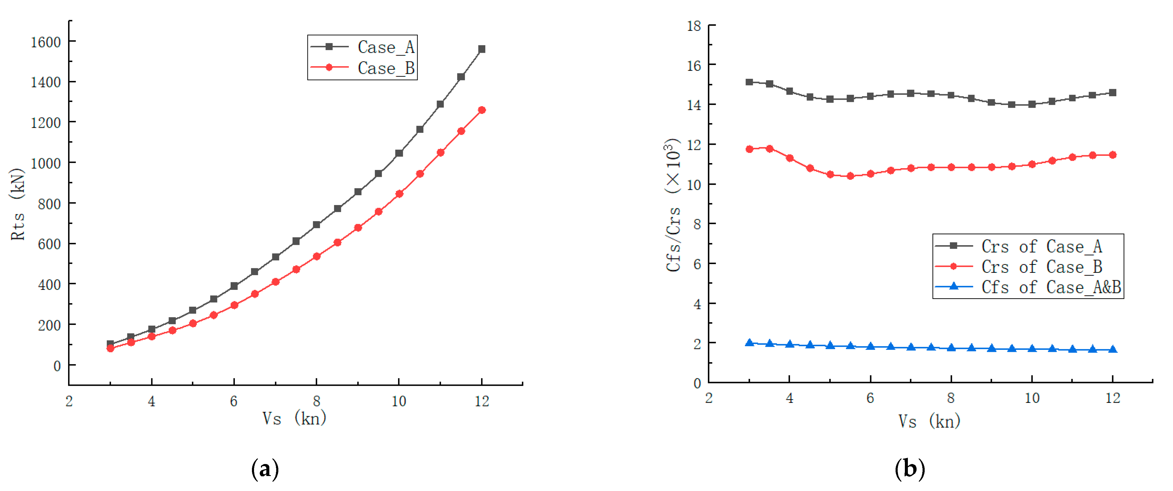
Resistance Components: The calm water resistance of WTIVs consists of frictional resistance, viscous pressure resistance, and wave-making resistance. Viscous pressure resistance accounts for over 65% of the total, followed by frictional resistance at approximately 12–15%, and wave-making resistance at 1–20%. As speed increases, the coefficients of viscous pressure resistance and frictional resistance decrease, while wave-making resistance increases due to pronounced bow and stern shoulder waves, particularly beyond 9.5 knots, where wave-making resistance rises sharply. The noticeable shoulder waves at the abrupt changes in the hull lines underscore the need to focus on viscous pressure resistance and wave-making resistance at higher design speeds. This observation aligns with the design speeds of 8–9 knots for similarly scaled WTIVs in China.

(2)

Impact of Spudcan Retraction Well Area on Resistance: Analysis of the resistance impact with and without spudcan retraction wells reveals a significant “moonpool additional resistance effect”, increasing the total calm water resistance by approximately 30% at design speed. Therefore, the design of such vessels should prioritize the matching of the spudcan structures with the hull shell plate to minimize gaps, maintain flow field continuity, reduce the adverse effects of the spudcan retraction well area on flow, and diminish eddy intensity in this region, thereby improving resistance performance.

(3)

Selection of Turbulence Models for Resistance Prediction: The selection of turbulence models for the target vessel at different speeds should be based on F_r = 0.15. For lower speeds (F_r ≤ 0.15), the SST k-ω turbulence model is more suitable for predicting the resistance of low-speed ships. For higher speeds (F_r > 0.15), the Realizable k-ε model with wall functions provides higher accuracy due to the fully developed turbulence around the hull at higher Reynolds numbers.

(4)

Modification of Resistance Calculation Based on the Holtrop Method: Compared to model tests and CFD analysis, the empirical formula estimation method, which integrates existing estimation formulas with operational vessel data, offers advantages such as time efficiency and cost-effectiveness. This is particularly beneficial in the preliminary design phase of ships, providing designers with quick resistance estimation results and relatively accurate references for ship propulsion configuration and speed estimation. This study incorporates resistance data from multiple operational WTIVs to modify the Holtrop-based resistance calculation formulas, resulting in empirical formulas suitable for full and blunt hull form self-elevating WTIVs, especially those with spudcan retraction wells.

Despite the insights presented, this study has certain limitations and areas that require further refinement. Firstly, regarding the empirical formula method, the current database of hull forms used in this study is limited in sample size. Therefore, it is imperative to continuously incorporate resistance data from other full-scale WTIVs in future research to expand and enhance the applicability and accuracy of the empirical formulas. Secondly, although calm water resistance constitutes the primary component of total resistance during actual ship operations, several factors unique to WTIVs in transit have been underexplored. Specifically, WTIVs often have long legs exceeding 100 m fully retracted above the baseline, and wind turbine equipment such as blades and towers are typically transported on weather decks. Along with additional large structures and equipment, like living quarters and cranes, these conditions result in significant windage areas for the entire vessel. Consequently, air resistance becomes a critical factor in resistance assessment for WTIVs, which cannot be overlooked. At present, most ship model tests primarily use the air resistance coefficient recommended by the 15th International Towing Tank Conference (ITTC) for rough estimates. However, there is a notable gap in research concerning the impact of wind loads on open truss structures, such as legs and crane booms, on the total resistance of WTIVs. This aspect represents a significant direction for future research in resistance optimization.

References

1. Huang, P.T.; Wu, Q.; Li, G.A.; Ma, Y.D.; Wang, W. Pratical Handbook for Ship Design; National Defense Industry Press: Beijing, China, 2013. [Google Scholar]
2. Kline, S. Describing uncertainty in single-sample experiments. Mech. Eng. 1953, 75, 3–8. [Google Scholar]
3. Guo, B.J.; Deng, G.B.; Steen, S. Verification and validation of numerical calculation of ship resistance and flow field of a large tanker. Ships Offshore Struct. 2013, 8, 3–14. [Google Scholar] [CrossRef]
4. Nikolov, M.; Judge, C. Uncertainty analysis for calm water tow tank measurements. J. Ship Res. 2017, 61, 177–197. [Google Scholar] [CrossRef]
5. Zhang, L.; Chen, J.T.; Chen, W.M.; Ma, X.Q. Uncertainty analysis of calibration ship model single-run resistance tests. Huazhong Univ. Sci. Technol. (Nat. Sci. Ed.) 2020, 48, 85–90. [Google Scholar]
6. Liu, H.; Ma, N.; Gu, X. Uncertainty analysis for ship-bank interaction tests in a circulating water channel. China Ocean Eng. 2020, 34, 352–361. [Google Scholar] [CrossRef]
7. ITTC. Recommended procedures and guidelines, 7.5-03-02-03, Practical guidelines for ship CFD applications. In Proceedings of the International Towing Tank Conference, Virtual, 13–18 June 2021. [Google Scholar]
8. Wu, C.S.; Qiu, G.Y.; Wei, Z.; Jin, Z.J. Uncertainty analysis on numerical computation of ship model resistance. J. Ship Mech. 2015, 19, 1197–1208. [Google Scholar]
9. Wang, Z.; Liu, X.; Zhang, S.; Xu, L.; Zhou, P. Uncertainty analysis in CFD for resistance. J. Shipp. Ocean Eng. 2017, 7, 192–202. [Google Scholar]
10. Islam, H.; Soares, C.G. Uncertainty analysis in ship resistance prediction using OpenFOAM. Ocean Eng. 2019, 191, 105805. [Google Scholar] [CrossRef]
11. Tong, S.L.; Chen, Z.G. Uncertainty analysis of ship model resistance measurement in circulating water channel. Chin. J. Ship Res. 2020, 15, 144–152. [Google Scholar]
12. Zhang, L.; Chen, W.; Chen, J.; Zhou, C. Verification and validation of CFD un-certainty analysis based on SST k-ω model. In Proceedings of the International Conference on Offshore Mechanics and Arctic Engineering (OMAE), Virtual, 3–7 August 2020; p. V008T008A044. [Google Scholar]
13. Zhang, L.; Zhou, C.M.; Chen, W.M.; Chen, J.T. Uncertainty Analysis of CFD Results of Standard Ship Model Resistance. Ship Ocean Eng. 2020, 49, 33–36. [Google Scholar]
14. Pena, B.; Huang, L. A review on the turbulence modelling strategy for ship hydrodynamic simulations. Ocean Eng. 2021, 241, 110082. [Google Scholar] [CrossRef]
15. Bojovic, P. Resistance of AMECRC systematic series of high speed displacement hull forms. In The IV Symposium on High Speed Marine Vehicles, Naples, Italy, 18–21 March 1997; Australian Maritime Engineering: Launceston, Australia, 1997. [Google Scholar]
16. Radojcic, D.; Zgradic, A.; Kalajdzic, M.; Simic, A. Resistance prediction for hard chine hulls in the pre-planing regime. Pol. Marit. Res. 2014, 21, 9–26. [Google Scholar] [CrossRef]
17. Xu, C. Optimization and Hydrodynamic Study of Wind Turbine Installation Vessel. Master’s Thesis, Harbin Engineering University, Harbin, China, 2016. [Google Scholar]
18. Huang, Y.N.; Chen, M.L.; Si, M.; Li, F.H.; Feng, J. Optimization of resistance reduction of offshore wind turbine installation vessel based on free-form deformation technique. J. Dalian Univ. Technol. 2023, 63, 61–68. [Google Scholar]
19. Kang, Z.; Xu, X.; Ni, W.; Zhang, C. Hydrodynamic Analysis and Model Test Study of Wind Turbine Installation Vessel. In Proceedings of the Twenty-Seventh (2017) International Ocean and Polar Engineering Conference IOPE 2017, San Francisco, CA, USA, 25–30 June 2017; pp. 767–774. [Google Scholar]
20. Jing, S.H. Self-Propelled Test and Resistance Numerical Analysis of Jack-Up Platform. Master’s Thesis, Jiangsu University of Science and Technology, Zhenjiang, China, June 2023. [Google Scholar]
21. Kjær, R.B.; Shao, Y.; Walther, J.H. Experimental and CFD analysis of roll damping of a wind turbine installation vessel. Appl. Ocean. Res. 2024, 143, 103857. [Google Scholar] [CrossRef]
22. Menter, F.R. Influence of Free stream Values on k-ω Turbulence Model Predictions. Aiaa J. 1992, 30, 1657–1659. [Google Scholar] [CrossRef]
23. Xia, G.Z. Ship Fluid Mechanics; Huazhong University of Science and Technology Press: Wuhan, China, 2003. [Google Scholar]
24. Yi, W.B.; Wang, Y.S.; Peng, Y.L.; Li, C.J. Resistance and flow field prediction of ship model with consideration of voyage attitude. J. Nav. Univ. Eng. 2016, 28, 26–30. [Google Scholar]
25. Holtrop, J.; Mennen, G. An Approximate Power Prediction Method; International Shipbuilding Progress: Amsterdam, The Netherlands, 1978. [Google Scholar]
26. Julianto, R.; Prabowo, A.; Muhayat, N.; Putranto, T.; Adiputra, R. Investigation of hull design to quantify resistance criteria using Holtrop’s regression-based method and Savitsky’s mathematical model: A study case of fishing vessels. J. Eng. Sci. Technol. 2021, 16, 1426–1443. [Google Scholar]
27. Nikolopoulos, L.; Boulougouris, E. A study on the statistical calibration of the Holtrop and Mennen approximate power prediction method for full hull form, low Froude number vessels. J. Ship Prod. Des. 2019, 35, 41–68. [Google Scholar] [CrossRef]
28. Crudu, L.; Bosoancă, R.; Obreja, D. A comparative review of the resistance of a 37,000 dwt Chemical Tanker based on experimental tests and calculations. Tech. Rom. J. Appl. Sci. Technol. 2020, 1, 59–66. [Google Scholar]
29. Wang, N.; Zhou, Z. Analysis of Improved Ship Resistance Holtrop Prediction Method. Ship Ocean Eng. 2019, 8, 34–37. [Google Scholar]
30. Sheng, Z.B.; Liu, Y.Z. Principles of Ship Design; Shanghai Jiao Tong University Press: Shanghai China, 2017; ISBN 978-7-313-17996-8/U661. [Google Scholar]
31. Hu, J.M. Study on Ship Powering Performance Prediction Based on Virtual Experimental Tank of RANS Method. Ph.D. Thesis, Dalian University of Technology, Dalian, China, 2018. [Google Scholar]
32. Deng, R. Numerical Research on Influence of the Interceptor on Catamaran Hydrodynamic Performances. Ph.D. Thesis, Harbin Engineering University, Harbin, China, 2010. [Google Scholar]
33. Duan, F.; Ma, N.; Zhang, L.J.; Cao, K.; Zhang, Q. Research on the influence of the moonpool scale effect on the navigation resistance of drilling ships. J. Ship Mech. 2020, 24, 1254–1260. [Google Scholar]
34. Lin, Y.; He, J.Y. Prediction of Ship Resistance and Free Motion Based on RANS Method. Ship Eng. 2019, 41, 52–57. [Google Scholar]
Figure 1. (a) The old generation WTIVs. (b) The new generation WTIVs.
Jmse 12 01337 g001
Figure 2. (a) The T-BOW hull line plan of WTIV_N. (b) The boundary layer trip and tunnel structure of WTIV_N. (c) The overview of the test model of WTIV_N.
Jmse 12 01337 g002
Figure 3. (a) Hull geometric surface model. (b) Computation domain and boundary condition of numerical simulation towing tank. (c) Local mesh refinement of WTIV spudcan and appendage surfaces. (d) Mesh division of calm water navigation fluid domain.
Jmse 12 01337 g003
Figure 4. (a) Spudcan is totally above the baseline. (b) The lower edges of the Spudcan are aligned with the baseline.
Jmse 12 01337 g004
Figure 5. (a) Comparison of total resistance between Case_A and Case_B. (b) Comparison of resistance coefficients between Case_A and Case_B.
Jmse 12 01337 g005
Figure 6. (a) Determination of form factor of Case_B. (b) Resistance coefficient of full-scale vessel. (c) Resistance components of full-scale vessel under different velocity. (d) The side view of the wave shape at bow area under speed 7 kn.
Jmse 12 01337 g006
Figure 7. (a) Time history curve of resistance with different grid sizes. (b) Time history curve of resistance with different turbulence models. (c) Comparison of wave elevation contours with different grid sizes. (d) Comparison of eddy strength distribution with different turbulence models.
Jmse 12 01337 g007
Figure 8. (a) Constrained streamlines on bow in Model test. (b) Constrained streamlines on bow in CFD. (c) Constrained streamlines on bilge in Model test. (d) Constrained streamlines on bilge in CFD. (e) Constrained streamlines on stern in Model test. (f) Constrained streamlines on stern in CFD.
Jmse 12 01337 g008aJmse 12 01337 g008b
Figure 9. (a) Wave elevation contours of stern by CFD (speed 7 kn). (b) Wave elevation contours of stern by experiment (speed 7 kn). (c) Pressure contours of stern (speed 5 kn). (d) Pressure contours of stern (speed 11 kn). (e) Pressure contours of bow (speed 5 kn). (f) Pressure contours of bow (speed 11 kn). (g) Constrained streamlines in Spudcan area of Case_A (speed 7 kn). (h) Constrained streamlines in Spudcan area of Case_B (speed 7 kn). (i) Hull eddy strength distribution of Case_A (speed 7 kn). (j) Hull eddy strength distribution of Case_B (speed 7 kn).
Jmse 12 01337 g009aJmse 12 01337 g009b
Figure 10. (a) Wave elevation contours comparison of model test and CFD (speed 5 kn). (b) Wave elevation contours comparison of model test and CFD (speed 7 kn). (c) Wave elevation contours comparison of model test and CFD (speed 10 kn).
Jmse 12 01337 g010aJmse 12 01337 g010b
Figure 11. (a) The view of the optimal spudcan retraction well in the side area. (b) The picture of the spudcan retraction well of the test model. (c) The view of the optimal horizontal line of the bow. (d) The view of the optimal buttock line of the bow.
Jmse 12 01337 g011
Figure 12. (a) Comparison of frictional resistance coefficients between WTIV_O&N. (b) Comparison of residual resistance coefficients between WTIV_O&N. (c) Comparison of constrained streamlines in bow area between WTIV_O&N (speed 9 kn). (d) Comparison of constrained streamlines in bottom area between WTIV_O&N (speed 9 kn). (e) Comparison of constrained streamlines in stern area between WTIV_O&N (speed 9 kn). (f) Comparison of constrained streamlines in spudcan area between WTIV_O&N (speed 9 kn). (g) Hull eddy strength distribution between of WTIV_O (speed 9 kn). (h) Hull eddy strength distribution of WTIV_N (speed 9 kn).
Jmse 12 01337 g012aJmse 12 01337 g012b
Figure 13. (a) Comparison of resistance components value between experimental and empirical formulas. (b) Speed prediction based on resistance and effective thrust curve.
Jmse 12 01337 g013