Abstract
The dynamic changes of sea ice exhibit spatial clustering, and this clustering has characteristics extending from its origin, through its development, and to its dissipation. Current research on sea ice change primarily focuses on spatiotemporal variation trends and remote correlation analysis, and lacks an analysis of spatiotemporal evolution characteristics. This study utilized monthly sea ice concentration (SIC) data from the National Snow and Ice Data Center (NSIDC) for the period from 1979 to 2022, utilizing classical spatiotemporal clustering algorithms to analyze the clustering patterns and evolutionary characteristics of SIC anomalies in key Arctic regions. The results revealed that the central-western region of the Barents Sea was a critical area where SIC anomaly evolutionary behaviors were concentrated and persisted for longer durations. The relationship between the intensity and duration of SIC anomaly events was nonlinear. A positive correlation was observed for shorter durations, while a negative correlation was noted for longer durations. Anomalies predominantly occurred in December, with complex evolution happening in April and May of the following year, and concluded in July. Evolutionary state transitions mainly occurred in the Barents Sea. These transitions included shifts from the origin state in the northwestern margin to the dissipation state in the central-north Barents Sea, from the origin state in the central-north to the dissipation state in the central-south, and from the origin state in the northeastern to the dissipation state in the central-south Barents Sea and southeastern Kara Sea. Various evolutionary states were observed in the same area on the southwest edge of the Barents Sea. These findings provide insights into the evolutionary mechanism of sea ice anomalies.
1. Introduction
Climate change has a profound impact on global water resources, food origin, and sea levels, making it the greatest environmental challenge facing humanity in the 21st century. In the context of global warming, sea ice serves as a sensitive indicator of climate change and plays a significant role in its effects [1]. The Arctic, also known as the “cold pole” of the Earth, has extensive sea ice coverage and experiences significant year-to-year variability, greatly impacting both local and global climate [2]. Since the 1990s, there has been a drastic decline in Arctic sea ice extent. In the summer of 2007, the minimum sea ice extent was 40% lower than the long-term average of 2005, nearly twice the historical record. This record was surpassed again in 2012 [3]. This has led to speculation about the existence of a critical point for Arctic sea ice, beyond which irreversible changes in the ice cover may lead to ice-free Arctic summers [4].
Existing studies on the spatiotemporal analysis of Arctic sea ice have primarily focused on trends and remote correlations. For example, Yang et al. [5] conducted a spatiotemporal analysis on monthly mean SIC and its trends across different Arctic regions. Their findings revealed that the highest and lowest concentrations occurred in March and September, respectively, with the Kara Sea showing the strongest melting trend. Similarly, Zhang et al. [6] analyzed SIC data from 14 significant straits in the Northeast Passage and Northwest Passage and concluded that, on an annual scale, the SIC in most straits was decreasing, with the exception of the Bering Strait and the Dmitry Laptev Strait. Pang et al. [7] also studied sea ice conditions in the Northeast Passage, specifically from July to October between 2002 and 2021. Their research demonstrated a significant improvement in navigability, supported by the decreasing trends in SIC and extent. Additionally, Liu et al. [8] investigated the spatiotemporal changes of sea ice in the Beaufort Sea from 1978 to 2015 and observed a decreasing trend in SIC with pronounced seasonal variations.
In recent decades, the Arctic has experienced rapid warming and a continuous reduction of sea ice. This has led to significant impacts on climate events in mid-latitudes, as the interaction and feedback processes between Arctic sea ice changes and the atmosphere have become more pronounced. For example, Li et al. [9] found that during the warming hiatus period from 1998 to 2013, changes in sea ice in the Barents–Kara Seas could explain 61.4% of the downward trend and 14.4% of the interannual variability in surface air temperature over China. This suggests that the accelerated melting of Arctic sea ice may have played a significant role in the intermittent warming observed in China over the past two decades. Additionally, Sun et al. [10] used statistical analysis of observational and reanalysis data to identify sea ice anomalies in winter in the Barents–Kara Seas as the dominant mode of interannual variability in extreme high-temperature events in spring across Eurasia in recent years. This finding allows for the possibility of seasonal forecasts of extreme events in advance. Furthermore, Shen et al. [11] pointed out that the positive and negative sea ice area anomalies over the Barents–Kara Seas in 1998 and 2016 may have caused differences in August precipitation in eastern China during these two periods. Shen also elucidated the possible mechanisms behind these differences.
Compared to traditional methods that use discrete variables, such as monthly or yearly averages, to analyze changes in sea ice, spatiotemporal clustering allows for a more effective capture of both temporal and spatial information, as well as complex structures within the data. This approach provides a more comprehensive and accurate representation of the distribution of anomalies. The goal of this study is to utilize classical spatiotemporal clustering methods to extract anomaly events in SIC and investigate the evolution of these anomalies. The aim is to gain a deeper understanding of the spatiotemporal distribution characteristics of SIC anomalies in the Arctic. The findings of this study will contribute to the development of regional climate variation theories, enhance our understanding of the dynamic characteristics of the Arctic sea ice system, and provide scientific evidence to address the challenges posed by climate change and sea ice retreat.
2. Materials and Methods
2.1. SIC Data
The SIC data used in this study were sourced from the NSIDC, and comprised daily gridded data. The NSIDC dataset is derived from a combination of data collected by the Nimbus-7 satellite’s scanning multichannel microwave radiometer and special sensors from the U.S. Defense Meteorological Satellite Program. The inversion algorithms used are a combination of the NASA Team algorithm and the NASA Bootstrap algorithm [12,13]. The dataset covers the Arctic region and provides daily and monthly SIC with a horizontal resolution of 25 × 25 km from 1978 to the present. After undergoing quality control and data correction processes by NSIDC, the SIC values have been standardized to a range of 0–100%. Missing values, such as those for land areas, have been excluded from the dataset.
This study analyzed SIC data from 1979 to 2022 for the entire Arctic region. The climatological state was determined by calculating the 44-year mean SIC, which served as a reference for identifying anomalies. SIC anomalies were then calculated by subtracting the climatological state from the original data. To identify regions with the most significant changes, trends in SIC variation were computed for each sea area on a monthly scale. These regions were designated as key Arctic regions. To further understand the distribution of SIC anomalies, spatiotemporal clustering was applied to the key regions. This allowed for the extraction of SIC anomaly events and provided insight into the spatiotemporal characteristics of these anomalies.
2.2. Methods
2.2.1. Trend Analysis
The trend analysis method enables the examination of grid data within a specific region on a pixel-by-pixel basis over time. This allows for the calculation of the slope of changes in pixel data, resulting in the determination of their spatial distribution [14]. The formula for this calculation is as follows:
where i represents the year index, with i = 1, 2…, n; n represents the number of years, with a value of 44; and SICAi represents the SIC anomaly value for the i-th year of the grid cell to be calculated. If slope > 0, it indicates an increasing trend in SIC anomaly values; if slope < 0, it indicates a decreasing trend, while slope = 0 suggests no change. The larger the absolute value of the slope, the more pronounced the trend.
2.2.2. Spatiotemporal Clustering
The ST-DBSCAN clustering algorithm which was utilized in this study requires four input parameters: Eps1, Eps2, Minpts, and Δε. Eps1 is the spatial threshold based on the longitude and latitude of the SIC anomalies’ position, while Eps2 is the temporal threshold based on the time of SIC anomalies’ occurrence. Minpts represents the minimum number of points within the distance ranges of Eps1 and Eps2, indicating that in dense regions, the number of points within the distance range should exceed the value of Minpts. The parameter Δε can also be used to prevent the discovery of combined clusters when the difference in non-spatial attribute values between adjacent locations is small. It is an optional parameter. The parameters can be determined through heuristic methods. The output of the algorithm is the cluster label for each object in the dataset.
To run the algorithm, it is necessary to clarify several definitions [15]:
- (1)
- Directly density-reachable.
An object p is directly density-reachable from the object q if p is within the Eps-neighborhood of q, and q is a core object.
- (2)
- Density-reachable.
An object p is density-reachable from the object q with respect to Eps1, Eps2 and Minpts if there is a chain of objects p1, …, pn, p1 = q and pn = q such that pi+1 is directly density-reachable from pi with respect to Eps1, Eps2 and Minpts, for 1 ≤ i ≤ n, pi ⊆ D.
- (3)
- Core object.
A core object is a point that must have at least a minimum number (Minpts) of other points within its neighborhood of a given radius (Eps1 and Eps2).
- (4)
- Border object.
An object p is a border object if it is not a core object but is density-reachable from a core object.
The algorithm process mainly consists of seven parts [16]:
- (1)
- The algorithm starts from the first object o1 in the dataset D.
- (2)
- After processing object o1, the algorithm selects the next object o2. If o2 does not belong to any cluster, the Retrieve_Neighbours function is called.
- (3)
- The function Retrieve_Neighbours(o2, Eps1, Eps2) returns objects within a distance less than that of Eps1 and Eps2 for object o2.
- (4)
- If the function returns fewer objects than Minpts, object o2 is defined as noise, as it does not have enough neighboring points to form a cluster.
- (5)
- Objects that have been labeled as noise may change in the next iteration if they are density-reachable from other objects in D. This change typically occurs at the bounder objects of clustered clusters. If oi is a core object, a new cluster is created.
- (6)
- All objects that are directly density-reachable from these core objects are also labeled with cluster tags. The algorithm uses stack-based iteration to gather density-reachable objects.
- (7)
- If an object is not labeled as noise or assigned to another cluster, and the difference between the mean of the current cluster and the new value is less than or equal to Δε, then it is labeled as part of the current cluster. After processing the current object, the algorithm selects the next object in D and repeats the above process until all objects are processed.
2.2.3. Cluster Validity
One method for evaluating clustering effectiveness is the silhouette index. The silhouette index ranges from −1 to 1. If the index value is close to 1, the object is well-clustered. If the value is around 0, the object is likely between two clusters. A negative value indicates the object might be in the wrong cluster. The formula for this calculation is as follows:
where s(i) represents the silhouette index, a(i) represents the average distance between point i and all points in A (the cluster where point i is located), and b(i) represents the average distance between point i to all points in a cluster other than A.
3. Results and Discussion
3.1. Determination of Key Areas and Hyperparameters
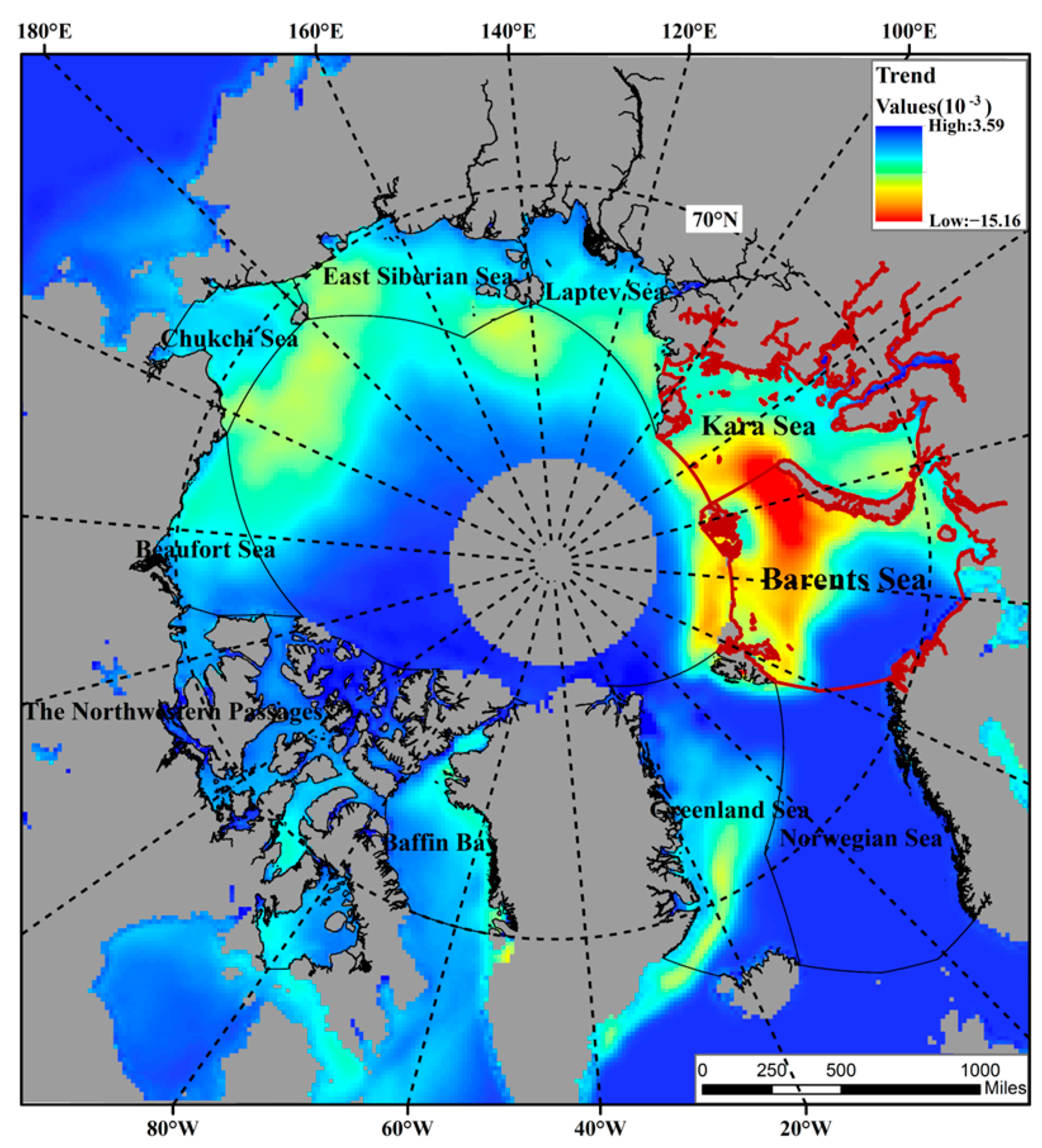
This study used SIC anomaly values from the entire Arctic region to create spatial distribution maps of changes in trends in different regions from 1979 to 2022 using formula (1), as depicted in Figure 1. The results indicate that the Barents–Kara Seas experienced the most significant anomalous changes and can be considered the key area in the Arctic.

Figure 1.
Map of the distribution trends of SIC anomalies in different Arctic regions.
Before implementing the ST-DBSCAN clustering algorithm, it is necessary to establish the appropriate values for the spatial distance parameter (Eps1), temporal distance parameter (Eps2), and cluster density (Minpts). In this study, the hyperparameter determination method used by Iswari was referenced [16]. The first step was to determine the optimal spatial threshold (Eps1) using a distance graph. This method involves calculating the spatial distances between point objects, sorting the results in descending order, and plotting them as a point–line graph. The optimal threshold is identified at the point where the most significant change occurs on the graph. Based on this method, the elbow curve of the Eps1 distance sequence in this study was found to be between 0.5 and 2.0 degrees.
Secondly, DBSCAN clustering was applied to determine the value of Minpts. By testing different values of Minpts using various values of Eps1 with an interval of 0.2 degrees, the main clusters with significant density can be identified. In this study, the value of Minpts was set to range from 3 to 10. The silhouette index was used to evaluate the DBSCAN clustering results, and the Eps1 and Minpts values corresponding to the highest silhouette index were selected as the input parameters.
Based on the information provided in Table 1, it can be concluded that the highest silhouette index value was 0.47, which was achieved with an Eps1 value of 1.05 and a Minpts value of 3. The Eps2 parameter was determined by setting a range of 2 to 8 days for clustering, and the highest silhouette index value was obtained with an Eps2 value of 7. Therefore, the input parameters for ST-DBSCAN were determined to be Eps1 = 1.05, Eps2 = 7, Minpts = 3, and the optional parameter Δε = 2.

Table 1.
Silhouette index of several combinations.
3.2. Spatiotemporal Clustering Patterns of SIC Anomalies
The ST-DBSCAN model was utilized to analyze the dataset of SIC anomalies from January 1979 to December 2022. This allowed for the identification of monthly SIC anomalies and the main spatiotemporal clusters representing the distributions of these anomalies. Based on the duration and evolution characteristics of these clusters, this study defined an SIC anomaly event as an anomalously high event that exceeds the climatological state of the SIC for more than five consecutive months and exhibits a complete lifecycle process, from origin through development or complex evolutionary behaviors to dissipation. To further understand the intensity and impact of these events, the Strength of Spatiotemporal Cluster (SSTC) was defined as the product of the area and the SIC anomaly average value of the spatiotemporal cluster for each month [17]. The calculation formula is as follows:
where n represents all months of the spatiotemporal cluster, Sti denotes the strength of the main spatiotemporal cluster in month ti, Ati represents the area of the main spatiotemporal cluster, and Rti denotes the SIC anomaly average value of the main spatiotemporal cluster at that time.
For the purpose of convenience in describing the evolution of SIC anomaly events, six types of states were defined:
- (1)
- Origin State.
This state occurs when there is no preceding main spatiotemporal cluster connected to the SIC anomaly object. It represents the initial stage of an SIC anomaly event, indicating the emergence of a new SIC anomaly.
- (2)
- Development State.
This state occurs when an SIC anomaly object has a connected main spatiotemporal cluster in both the preceding and subsequent time steps. It signifies the continued evolution and persistence of the SIC anomaly over time.
- (3)
- Dissipation State.
This state occurs when an SIC anomaly object is not connected to any main spatiotemporal cluster in the subsequent time step. It represents the end stage of the anomaly event, in which the anomaly dissipates and ceases to exist.
- (4)
- Merge State.
This state occurs when there are at least two main spatiotemporal clusters connected to the SIC anomaly object in the preceding time step, and only one main spatiotemporal cluster connected to it in the subsequent time step. It indicates the merging of multiple SIC anomaly objects into a single anomaly.
- (5)
- Split State.
This state occurs when an SIC anomaly object is connected to only one main spatiotemporal cluster in the preceding time step, but there are at least two main spatiotemporal clusters connected to it in the subsequent time step. It signifies the splitting of a single SIC anomaly into multiple anomalies.
- (6)
- Merge–Split State.
This state occurs when there are at least two main spatiotemporal clusters connected to the SIC anomaly object in both the preceding and subsequent time steps. It represents a complex interaction where the anomaly objects undergo both merging and splitting within the same time period.
For ease of expression, the latter three state types were referred to as complex state types, and the corresponding evolutionary behaviors as complex evolutionary behaviors.
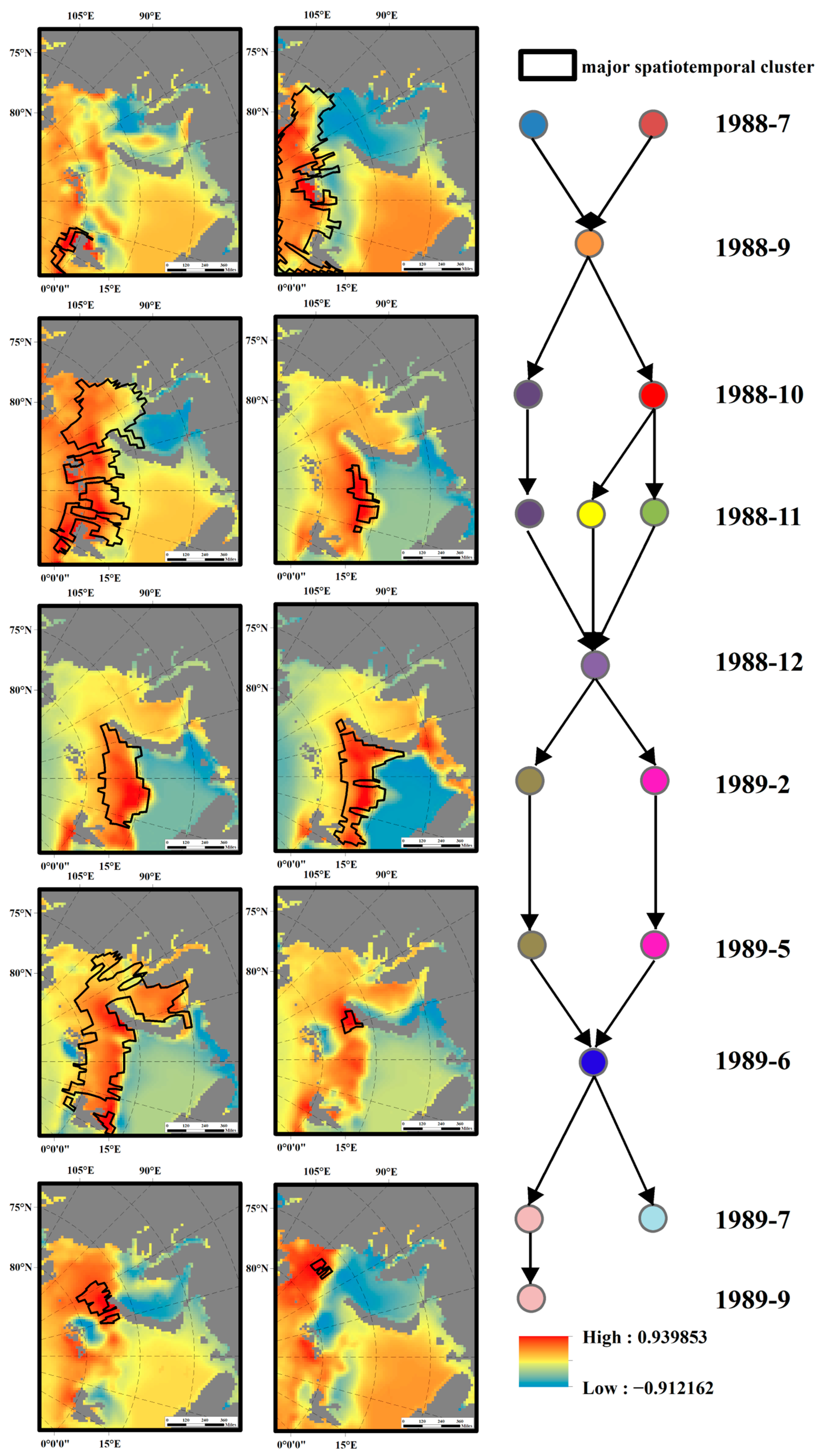
Based on the concepts discussed above, this study identified a total of 49 SIC anomaly events, with a minimum duration of 5 months and a maximum duration of 16 months. To better understand the patterns of these events, the maximum, minimum, average, and difference between the maximum and minimum values of SSTC and anomaly mean values were considered, along with the duration. An example of the evolution process, showing an event from July 1988 to September 1989, is illustrated in Figure 2. In the right part of the figure, circles of different colors represent various SIC anomaly objects, and the arrows indicate the evolution of these anomalies. The SIC anomaly event originated in July 1988 at two adjacent locations on the edge of the Barents Sea. Subsequently, in September 1988, these anomalies merged into a new SIC anomaly object. In October and November 1988, the anomaly object underwent consecutive splits and eventually re-merged in December 1988. Starting from May 1989, the anomaly object began to decay, experiencing various evolutionary behaviors such as merging and splitting, and eventually dissipating in the central Kara Sea in September 1989.
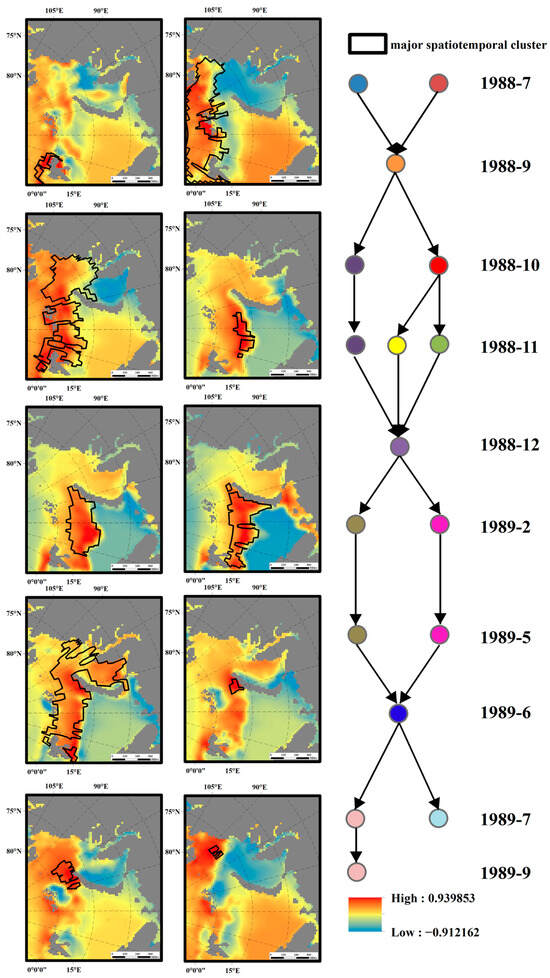
Figure 2.
Evolution process of an SIC anomaly event in the Barents–Kara Seas from July 1988 to September 1989.
The study analyzed the primary months of occurrence for the origin state, dissipation state, and complex evolutionary behavior of SIC anomaly events. SIC anomaly events mostly began to occur in December each year. In April of the following year, they were more likely to exhibit split or merge evolutionary behaviors, with merge–split behaviors being more prevalent in May. Dissipation states were more common in July.
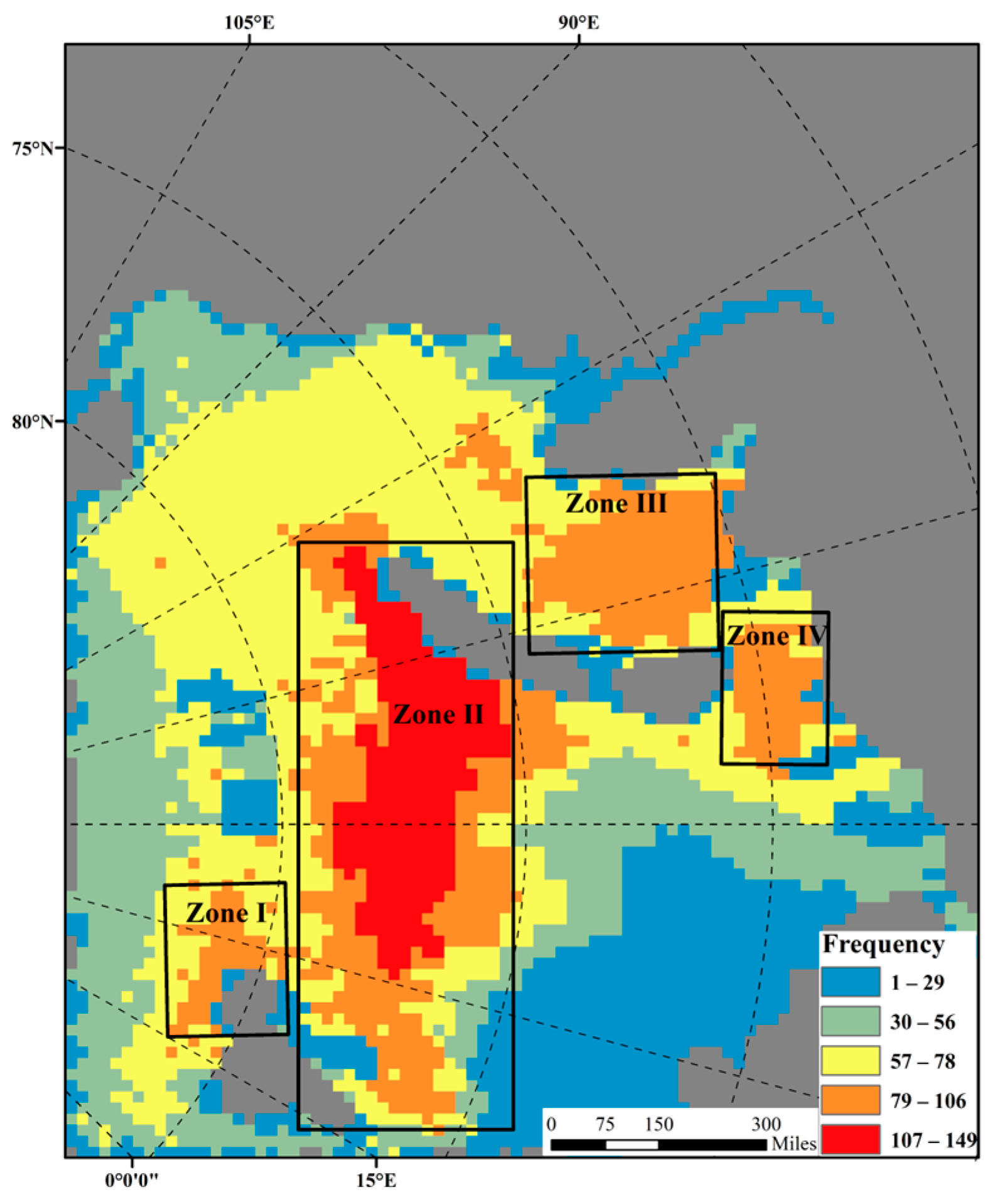
Based on the spatial distribution of spatiotemporal clusters, the frequency of SIC anomaly events from 1979 to 2022 was determined, and is illustrated in Figure 3. There were four key regions where anomaly events occurred frequently: the western edge of the Barents Sea (Zone I), the central-western part of the Barents Sea (Zone II), the northeastern part of the Kara Sea (Zone III), and the southeastern part of the Barents Sea (Zone IV).

Figure 3.
Spatial distribution of SIC anomaly event frequency in the Barents–Kara Seas.
The number of months with SIC anomaly events in four key regions was statistically analyzed, as shown in Figure 4. The average number of months with anomaly events in these regions, from longest to shortest, was as follows: Zone II > Zone I > Zone IV > Zone III. This indicates that not only were there more SIC anomaly events in Zone II, but they also spanned a longer period. The SSTC values and durations of SIC anomaly events in key regions were statistically analyzed, as shown in Figure 5. The analysis illustrates that the relationship between the intensity of SIC anomaly events and their duration was complex. Specifically, there appeared to be a positive correlation between intensity and duration for shorter durations (5–10 months), suggesting that events tended to become more intense as their duration increased within this range. Conversely, for longer durations (11–14 months), a negative correlation was observed, indicating that the intensity of events may decrease as their duration extends further. This trend underscored the non-linear nature of the relationship between the intensity and duration of SIC anomaly events, a relation which cannot be fully captured by a simple linear assessment.
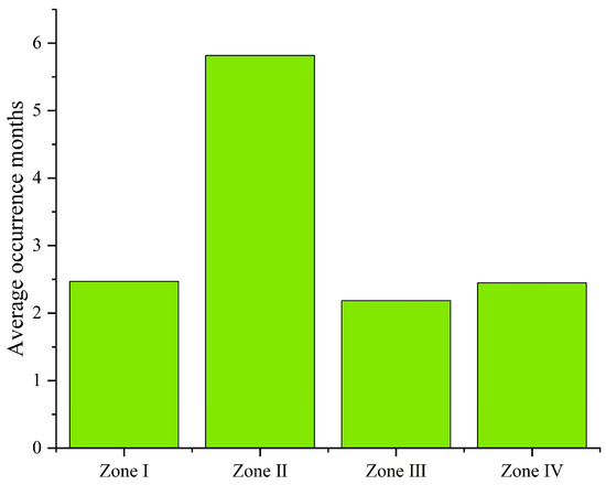
Figure 4.
The average number of months with SIC anomaly events in the four key regions.
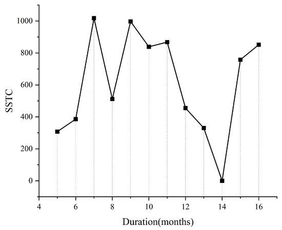
Figure 5.
Statistics on the duration and corresponding SSTC values of SIC anomaly events.
3.3. Spatial Transformation Characteristics of SIC Anomaly Evolution
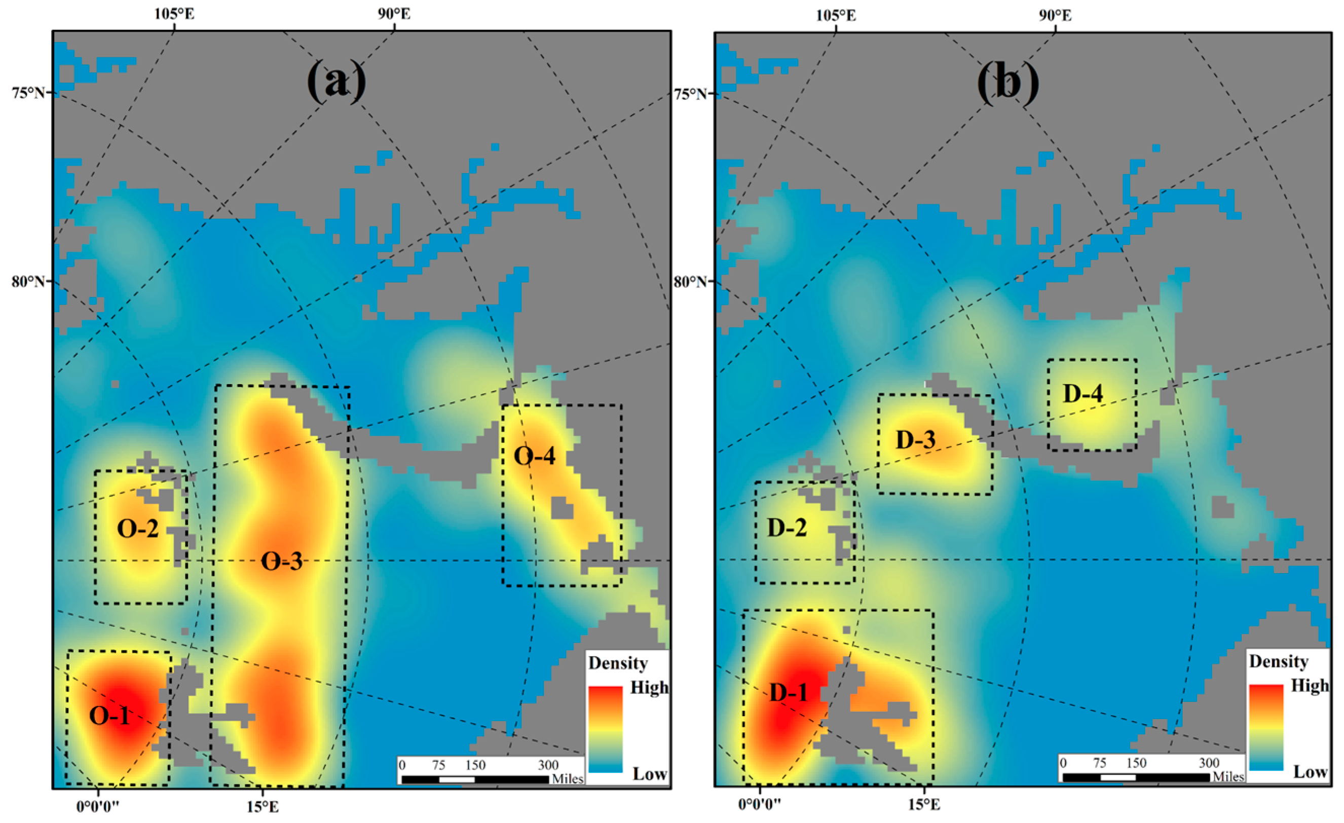
This study examined the spatial distribution characteristics of SIC anomaly events, including their origins, dissipations, and complex evolutionary behaviors such as splitting, merging, and merging–splitting. The centroid positions of each anomaly event were abstractly summarized and subjected to kernel density analysis. Figure 6 and Figure 7 display the results of this analysis, illustrating the major spatial distribution of origins, dissipations, and complex evolutionary behaviors in the Barents and Kara Seas. To facilitate discussion, this study combines the spatial locations of splitting, merging, and merging–splitting behaviors and refers to them as complex evolution zones.
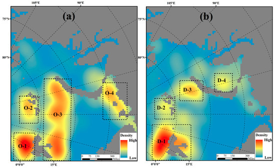
Figure 6.
The kernel density distribution of the (a) origin and (b) dissipation of SIC anomaly events in the Barents–Kara Seas.

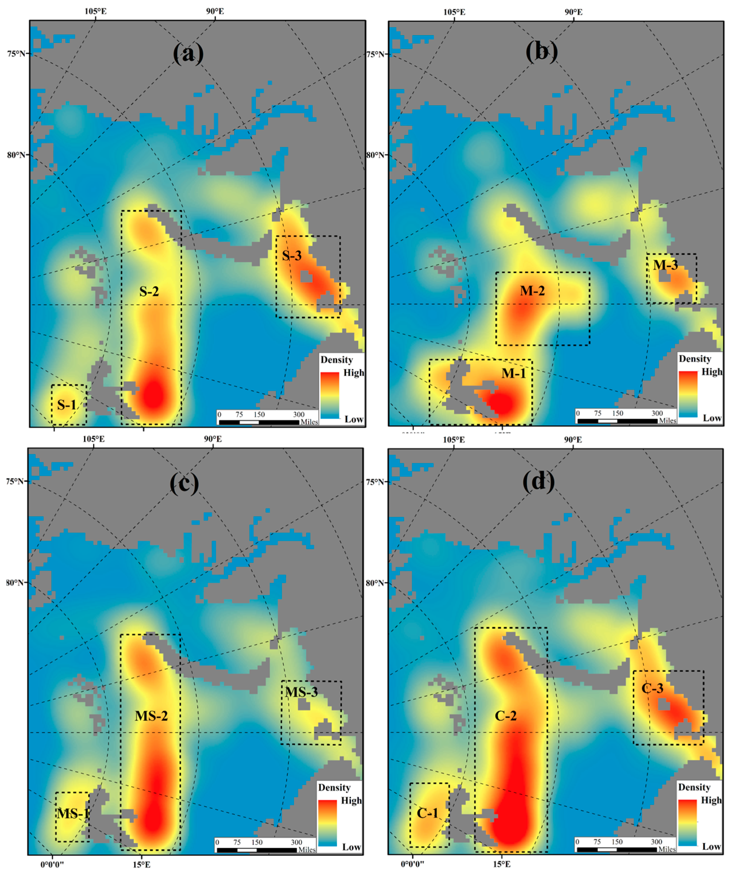
Figure 7.
The spatial distribution of complex evolutionary behaviors of SIC anomaly events in the Barents–Kara Seas: (a) splitting; (b) merging; (c) merging–splitting; (d) complex evolution zones.
From Figure 6, it can be seen that the distribution areas of origin and dissipation of SIC anomaly events in the western edge of the Barents Sea were roughly the same, with some overlap in the central region of the Barents Sea. Additionally, there were origins in the northeast part of the Barents Sea and dissipations in the southeast part of the Kara Sea. According to Figure 7, in the key regions, the splitting, merging, and merging–splitting evolutionary behaviors mainly occurred in three areas of the Barents Sea: the southwest edge (referred to as Zone C-1), the central region (referred to as Zone C-2), and the northeast edge (referred to as Zone C-3). Complex evolutionary behaviors were more frequent in Zone C-2, merging behaviors were more common in Zone C-1, and splitting behaviors were more common in Zone C-3. In summary, the regions where origins, dissipations, and complex evolutionary behaviors occurred were mainly located in the Barents Sea region, which is characterized by intense interactions between the atmosphere and the ocean. Under the combined influence of the dynamic processes of wind and ocean, SIC anomalies were forced to undergo various evolutionary behaviors in the mentioned areas.
To investigate the overall spatial transformation characteristics of SIC anomaly events in key sea areas, this study conducted a statistical analysis of the relationship between the origins and dissipations of these events in the main regions, as shown in Table 2. The percentages in the table represent the proportion of anomaly events originating from a specific origin and ending in various dissipations. For example, the relevant percentage in Table 2 indicates that the number of anomaly events originating in region O-1 and dissipated in region D-1 accounts for 45.45% of all anomaly events originating in region O-1. The corresponding 0.00% value in Table 2 indicates that none of the SIC anomaly events originating in region O-2 dissipated in region D-2. Furthermore, the study analyzed the complex evolutionary behaviors and distributions of origins and dissipations. To simplify the analysis, only the maximum or second-largest percentage value with a smaller difference from the maximum was selected for each row in the O-D table. Table 3 and Table 4 show the percentages of anomaly events with complex evolutionary behaviors originating from and dissipating in the designated areas, respectively. For instance, the percentage in Table 3 indicates that the events with complex evolutionary behaviors occurring in region C-1 and originating from region O-1 account for 33.33% of all events with complex evolutionary behaviors in region C-1.
Table 2.
The correspondence between origins and dissipations of abnormal events.
Table 3.
Distribution of abnormal events’ origins relative to the complex behavior area.
Table 4.
Distribution of abnormal events’ dissipations relative to the complex behavior area.
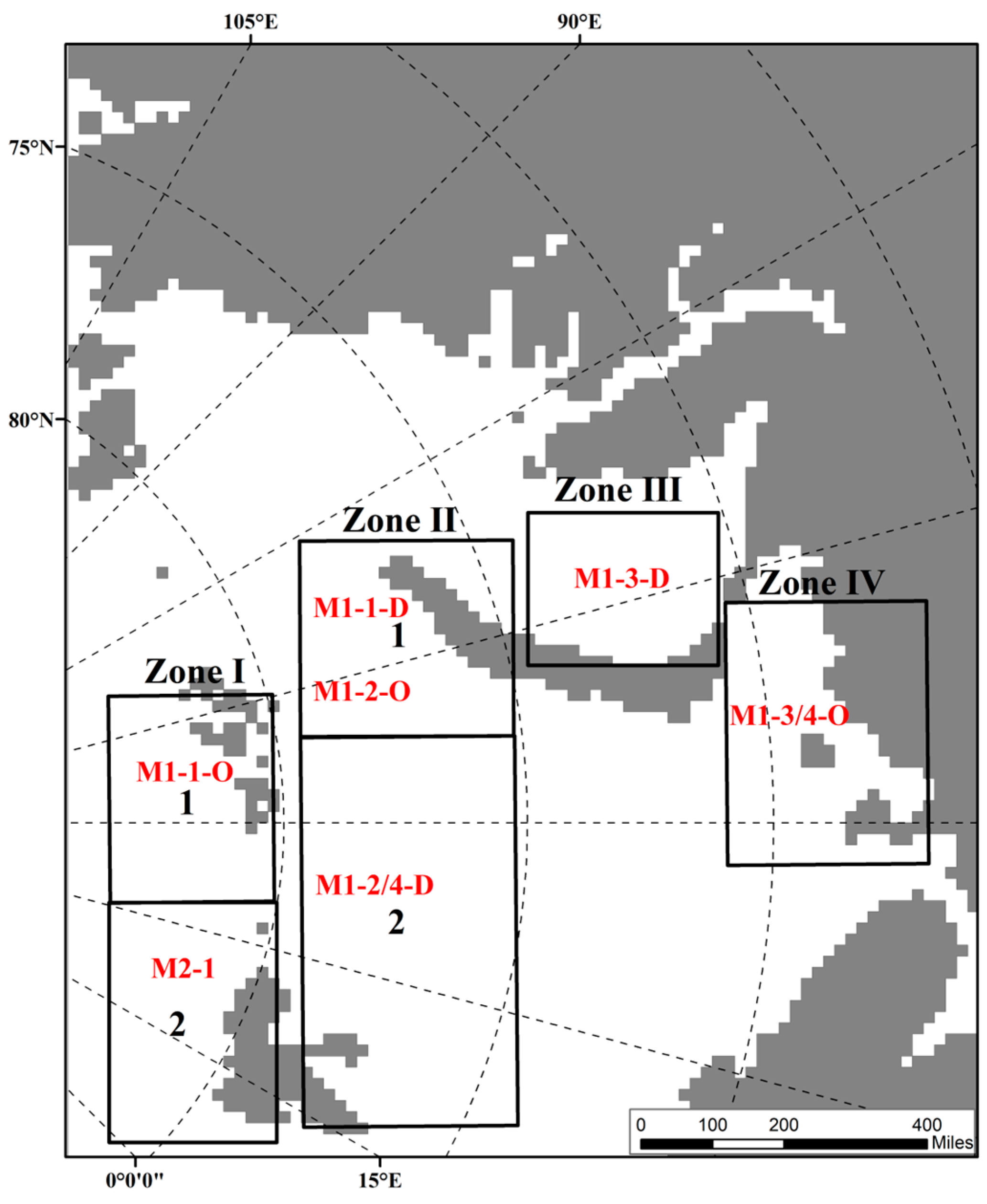
Based on the distribution results for evolutionary behaviors in Figure 6 and Figure 7, the key sea areas were divided into subregions based on the concentrated distribution areas of origins, complex evolutionary behaviors, and dissipations, as shown in Figure 8. Zone I and Zone II, along with their surrounding areas, were divided into two subregions denoted as Zone I-1 and Zone I-2, and Zone II-1 and Zone II-2. The Zone I-2 subregion experienced origins, complex evolutionary behaviors, and dissipations, with relatively fewer anomaly events undergoing complex evolutionary behaviors. Two spatial transformation patterns of SIC anomalies, M1 and M2, were defined. M1 represents anomaly events that involve multiple subregions, from origin through complex evolutionary behaviors, to dissipation, while M2 represents events that occur entirely within a single subregion (such as Zone I-2). Based on the statistical results from Table 2, Table 3 and Table 4 and the subdivision of subregions in Figure 8, the spatial transformation characteristics of SIC anomalies in each subregion were summarized. M1-1-O/D represents the origin/dissipation state of the first type of spatial transformation in the M1 pattern.
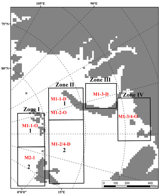
Figure 8.
Spatial transformation of SIC anomaly events in key sea areas.
From Figure 8, it can be observed that there were four types of spatial transformations for SIC anomaly events in the M1 pattern. Anomaly events originating from the origin state in Zone I-1 underwent a series of complex evolution processes before transitioning into the dissipation state in Zone II-1. Similarly, events originating from the origin state in Zone II-1 transitioned into the dissipation state in Zone II-2, while those originating from Zone IV and undergoing different evolution processes proceeded to the dissipation state in Zone III and Zone II-2. The state transitions of the M2 pattern occurred exclusively within Zone I-2. The transition from Zone I to Zone II might be associated with an increase in Atlantic heat transport, particularly with reference to the Barents Sea Opening Zone in the western part of the Barents Sea [18]. Additionally, the state transition in different subregions of Zone II might result from the interaction of polar-high latitude atmospheric circulation fields, driven by the combined effects of two wave trains passing through the Norwegian Sea–Eurasian continent–Arabian Peninsula and the Barents–Kara Seas [19]. The transition from Zone IV to Zone III was correlated with the decrease in accumulated SIC in the eastern Kara Sea [20]. Furthermore, the occurrence of anomaly events exhibited regional characteristics and internal interactions under the influence of local atmospheric forcing [21]. In cases where Arctic oscillations influence near-surface wind fields and ocean surface currents, a transition from the origin state in Zone IV to the dissipation state in Zone II-2 might occur [22].
4. Conclusions
This study conducted spatiotemporal cluster pattern mining of SIC anomalies in key Arctic sea areas based on NSIDC SIC data covering the time period from January 1979 to December 2022. Through the ST-DBSCAN method, the spatiotemporal evolutionary characteristics of SIC anomalies were analyzed. The following main conclusions were obtained.
Based on the ST-DBSCAN model, 49 complete life cycle SIC anomaly events occurring in the key Arctic regions, namely the Barents–Kara Seas, from 1979 to 2022, were extracted. Using the spatial distribution of occurrence frequency as a criterion, four key sea areas were identified: the western edge of the Barents Sea, the central-western part of the Barents Sea, the northeastern part of the Barents Sea, and the southeastern part of the Kara Sea. The central-western part of the Barents Sea was found to be more susceptible to evolutionary behaviors and exhibited longer durations. Within these four key sea areas, two categories and five types of state space transition patterns were identified. Furthermore, based on the statistical relationship between SSTC values and duration, it was observed that the intensity of SIC anomaly events did not simply increase with longer duration. Instead, a positive correlation was observed for shorter durations (5–10 months), while a negative correlation was noted for longer durations (11–14 months). This finding suggests that the factors driving the intensity of SIC anomaly events may change with their duration.
Analysis of the spatiotemporal distributions of SIC anomaly event origins, complex evolutionary behaviors, and dissipations in key sea areas revealed the following patterns: SIC anomaly events predominantly occurred in December of each year, underwent complex evolutionary behaviors in April and May of the following year, and dissipated in July. The spatial transformation patterns were as follows: anomaly events originating from the origin state in the northwestern edge of the Barents Sea transitioned to a dissipation state in the central-north part of the Barents Sea. Those originating from the origin state in the central-north part of the Barents Sea transitioned to dissipation state in the central-south part. Meanwhile, anomalies originating from the origin state in the northeastern part of the Barents Sea underwent different evolution processes, transitioning to dissipation state in the central-south part of the Barents Sea and the southeastern part of the Kara Sea. Anomaly events with varying evolutionary states had been observed in the southwest edge of the Barents Sea.
The spatiotemporal evolution characteristics of the SIC anomalies can provide valuable insights into analyzing the mechanisms underlying changes in sea ice anomalies. As the “cold pole” of the Northern Hemisphere, the variability of sea ice in the Arctic can significantly impact the climate change, not only in the Northern Hemisphere but also globally. Investigating the relationship and mechanisms between Arctic sea ice changes and climate variables such as temperature and precipitation in mid-to-high latitude regions through the exploration of ocean dynamics processes and ocean–atmosphere interaction coupling will have significant scientific implications.
Author Contributions
Y.L. (Yongheng Li) and Y.H. conceptualized this study; Y.L. (Yongheng Li) and Y.L. (Yanhua Liu) carried out this study and performed the calculations; Y.L. (Yongheng Li) drafted the paper; Y.L. (Yongheng Li), Y.H., Y.L. (Yanhua Liu) and F.J. processed the review and editing of the paper. All authors have read and agreed to the published version of the manuscript.
Funding
This study is supported by the National Natural Science Foundation of China (No. 4197060184).
Institutional Review Board Statement
Not applicable.
Informed Consent Statement
Not applicable.
Data Availability Statement
The data for Arctic sea ice concentration were obtained from the National Snow and Ice Data Center (https://nsidc.org/ (accessed on 17 April 2023)).
Conflicts of Interest
The authors declare no conflicts of interest.
References
- Wang, Z.; Li, Z.; Zeng, J.; Liang, S.; Zhang, P.; Tang, P.; Chen, S.; Ma, X. Spatial and Temporal Variations of Arctic Sea Ice from 2002 to 2017. Earth Space Sci. 2020, 7, e2020EA001278. [Google Scholar] [CrossRef]
- Zhang, P.; Wu, Z.; Jin, R. How can the winter North Atlantic Oscillation influence the early summer precipitation in Northeast Asia: Effect of the Arctic sea ice. Clim. Dyn. 2021, 56, 1989–2005. [Google Scholar] [CrossRef]
- Maksym, T. Arctic and Antarctic Sea Ice Change: Contrasts, Commonalities, and Causes. Annu. Rev. Mar. Sci. 2019, 11, 187–213. [Google Scholar] [CrossRef]
- Lenton, T.M.; Held, H.; Kriegler, E.; Hall, J.W.; Lucht, W.; Rahmstorf, S.; Schellnhuber, H.J. Tipping elements in the Earth’s climate system. Proc. Natl. Acad. Sci. USA 2008, 105, 1786–1793. [Google Scholar] [CrossRef]
- Yang, M.; Qiu, Y.; Huang, L.; Cheng, M.; Chen, J.; Cheng, B.; Jiang, Z. Changes in Sea Surface Temperature and Sea Ice Concentration in the Arctic Ocean over the Past Two Decades. Remote Sens. 2023, 15, 1095. [Google Scholar] [CrossRef]
- Zhang, T.; Huang, J.; Cao, Y.; Wang, L.; Sun, Y.; Yang, L. Spatiotemporal Variation of Sea Ice Concentration in Important Arctic Straits is Heterogeneous. Remote Sens. Technol. Appl. 2019, 34, 1162–1172. (In Chinese) [Google Scholar]
- Pang, X.; Zhang, C.; Ji, Q.; Chen, Y.; Zhen, Z.; Zhu, Y.; Yan, Z. Analysis of sea ice conditions and navigability in the Arctic Northeast Passage during the summer from 2002–2021. Geo-Spat. Inf. Sci. 2023, 26, 465–479. [Google Scholar] [CrossRef]
- Liu, Y.; Pang, X.; Zhao, X.; Su, C.; Ji, Q. Analysis of spatiotemporal variability of sea ice in the Beaufort Sea using passive microwave remote sensing data. Chin. J. Polar Res. 2018, 30, 161–172. (In Chinese) [Google Scholar] [CrossRef]
- Li, X.; Wu, Z.; Li, Y. A link of China warming hiatus with the winter sea ice loss in Barents–Kara Seas. Clim. Dyn. 2019, 53, 2625–2642. [Google Scholar] [CrossRef]
- Sun, J.; Liu, S.; Cohen, J.; Yu, S. Influence and prediction value of Arctic sea ice for spring Eurasian extreme heat events. Commun. Earth Environ. 2022, 3, 172. [Google Scholar] [CrossRef]
- Shen, H.; He, S.; Wang, H. Effect of Summer Arctic Sea Ice on the Reverse August Precipitation Anomaly in Eastern China between 1998 and 2016. J. Clim. 2019, 32, 3389–3407. [Google Scholar] [CrossRef]
- Tschudi, M.A.; Meier, W.N.; Stewart, J.S. An enhancement to sea ice motion and age products at the National Snow and Ice Data Center (NSIDC). Cryosphere 2020, 14, 1519–1536. [Google Scholar] [CrossRef]
- Liu, Q.; Zhang, R.; Wang, Y.; Yan, H.; Hong, M. Daily Prediction of the Arctic Sea Ice Concentration Using Reanalysis Data Based on a Convolutional LSTM Network. J. Mar. Sci. Eng. 2021, 9, 330. [Google Scholar] [CrossRef]
- Pang, X.; Liu, J. Effects of climate changes on the NDVI of vegetation in Asia. Remote Sens. Nat. Resour. 2023, 35, 295–305. (In Chinese) [Google Scholar]
- Birant, D.; Kut, A. ST-DBSCAN: An algorithm for clustering spatial–temporal data. Data Knowl. Eng. 2007, 60, 208–221. [Google Scholar] [CrossRef]
- Iswari, L. Profiling the Spatial and Temporal Properties of Earthquake Occurrences Using ST-DBSCAN Algorithm. In Proceedings of the IEEE 7th International Conference on Information Technology and Digital Applications (ICITDA), Yogyakarta, Indonesia, 4–5 November 2022; pp. 1–8. [Google Scholar] [CrossRef]
- Liu, J.; Xue, C.; He, Y.; Dong, Q.; Kong, F.; Hong, Y. Dual-Constraint Spatiotemporal Clustering Approach for Exploring Marine Anomaly Patterns Using Remote Sensing Products. IEEE J. Sel. Top. Appl. Earth Obs. Remote Sens. 2018, 11, 3963–3976. [Google Scholar] [CrossRef]
- Xie, T.; Zhang, Y.; Chen, C.; Xu, D.; Zhang, X.; Wang, Y.; Zhang, Y. Key processes of sea ice variation and thermodynamic response in the Barents Sea and Kara Sea. Adv. Mar. Sci. 2023, 41, 24–39. (In Chinese) [Google Scholar]
- Pan, Y.; Zhang, Y.; Li, S. Assessment of CMIP models in simulating the relationship between wintertime atmospheric circulation in the Northern Hemisphere and the winter-spring temperature over the Tibetan Plateau. J. Meteorol. Sci. 2022, 42, 440–456. (In Chinese) [Google Scholar]
- Wang, W.; Zhao, J. Accumulation Sea ice concentration and its action on understanding arctic sea ice dramatic change. Adv. Earth Sci. 2014, 29, 712–722. (In Chinese) [Google Scholar]
- Jacox, M.G.; Bograd, S.J.; Hazen, E.L.; Fiechter, J. Sensitivity of the California Current nutrient supply to wind, heat, and remote ocean forcing. Geophys. Res. Lett. 2015, 42, 5950–5957. [Google Scholar] [CrossRef]
- Qi, L.; Xu, Y. Interdecadal variations of Arctic sea ice and its interannual relationship with meteorological elements. Trans. Atmos. Sci. 2018, 41, 355–366. (In Chinese) [Google Scholar] [CrossRef]


Disclaimer/Publisher’s Note: The statements, opinions and data contained in all publications are solely those of the individual author(s) and contributor(s) and not of MDPI and/or the editor(s). MDPI and/or the editor(s) disclaim responsibility for any injury to people or property resulting from any ideas, methods, instructions or products referred to in the content. |
© 2024 by the authors. Licensee MDPI, Basel, Switzerland. This article is an open access article distributed under the terms and conditions of the Creative Commons Attribution (CC BY) license (https://creativecommons.org/licenses/by/4.0/).