Prescribed-Time Trajectory Tracking Control for Unmanned Surface Vessels with Prescribed Performance Considering Marine Environmental Interferences and Unmodeled Dynamics

Abstract

This article investigates a prescribed-time trajectory tracking control strategy for USVs considering marine environmental interferences and unmodeled dynamics. Firstly, a fixed-time extended state observer is introduced to quickly and accurately observe the compound perturbations including ocean disturbances and unmodeled dynamics. Subsequently, a prescribed-time prescribed performance function is utilized to obtain guaranteed transient performance within a predefined time. Finally, combining the fixed-time extended state observer, dynamic surface control technique, and prescribed-time prescribed performance control, a prescribed-time prescribed performance control strategy is developed to guarantee that the tracking errors converge to a predefined performance constraint boundary within a prescribed time. The effectiveness and superiority of the presented control strategy is verified by the simulation results.

1. Introduction

Due to the increasing demands for various tasks such as reconnaissance and surveillance, maritime rescue, hydrographic surveying and charting, and ocean resource development, as well as the improvement in task accuracy requirements, unmanned surface vessels (USVs) with high autonomy are playing an increasingly important role in both military and civilian fields [1,2]. Trajectory tracking, as one of the essential components of USV motion control, differs from path-tracking tasks. Trajectory tracking involves following a time-varying path through the dynamic system of USVs, which has strict requirements on time. The trajectory tracking control system often determines the success of various marine tasks. However, it is well known that USVs are affected by complex and unknown ocean disturbances, and the model has strong coupling and nonlinear characteristics. This brings significant challenges to the controller design of USV trajectory tracking. Additionally, different scenarios and task objectives impose higher performance requirements on the controller [3,4].

Currently, a variety of control approaches have been applied to the design of USV tracking controllers, such as backstepping control [5,6], sliding mode control [7,8], robust adaptive control [9,10], and model predictive control [11,12]. For underactuated USVs with system uncertainties and thrust saturation, an adaptive sliding mode control strategy uses a sliding mode control, neural networks, and backstepping technology [13] to guarantee that tracking errors asymptotically converge to the equilibrium point. Reference [14] studied the integral sliding mode control of USV tracking issues with unknown dynamics and proposed an adaptive neural network controller to provide robustness and adaptability. Considering USVs with model uncertainty and complex ocean disturbance, [15] used nonlinear gain sliding mode and an adaptive neural network to design a tracking controller and achieved excellent trajectory tracking performance. Combining super-twisting sliding mode technology and model predictive control algorithm, a robust model predictive control based on super-twisting sliding mode algorithm is designed in [16], which is used for USV trajectory tracking under system uncertainties and ocean interferences, and further improves the tracking accuracy of system. However, the control strategies above can only achieve asymptotic or exponential stability and fail to fulfill the requirements of USVs for performing complex tasks. In this context, finite-time trajectory tracking has developed into a research hotspot in motion control of USVs. In addition, finite-time control has a rapid convergence rate, high precision, and robust anti-jamming capability [17,18]. In [19], an adaptive control algorithm is suggested to address the issue of USV trajectory tracking with environmental disturbance and unknown system dynamics, guaranteeing the finite-time convergence of tracking errors. In [20], the trajectory tracking control problem of underactuated USVs with saturation constraints and model uncertainty is studied. A robust finite-time controller is developed to ensure the finite-time stability of all signals in the closed-loop system. Although the finite-time control method has obvious advantages, its convergence time depends on the initial conditions of the system. Hence, researchers have improved the finite-time control method and proposed the concept of fixed-time control [21,22]. For the issue of USV trajectory tracking with marine environment interference and model uncertainty, a fixed-time sliding mode scheme is proposed in [23], which ensures the convergence of tracking errors within a fixed time. In addition, to achieve guaranteed steady-state performance, [24] designed a fixed-time predefined performance tracking strategy, which further improves the tracking accuracy of USVs.

Since the stability time of fixed-time theory depends on complex control parameters, the controller design becomes more sophisticated. To simplify the controller design and ensure fast convergence and high precision, ref. [25] proposed a prescribed-time control theory. In [26], combining the prescribed-time algorithm and the prescribed performance technique, an AUV prescribed-time trajectory tracking control method is proposed, which enables tracking errors to be stable within a prescribed time and the stability time can be preset in advance by users. Furthermore, ref. [27] developed a USV prescribed-time control algorithm based on a prescribed-time perturbation observer, which makes the tracking error converge to the predefined performance constraint within a preset time. However, the interference observer designed in [27] cannot deal with the USV trajectory tracking control considering the unknown system dynamics.

Motivated by the discussions above, this article designed a high-precision trajectory tracking control scheme for USVs under unmodeled dynamics, marine environmental interferences, and thruster saturation constraints based on a fixed-time extended state observer and prescribed-time prescribed performance technique. The main contributions are threefold:

(1)

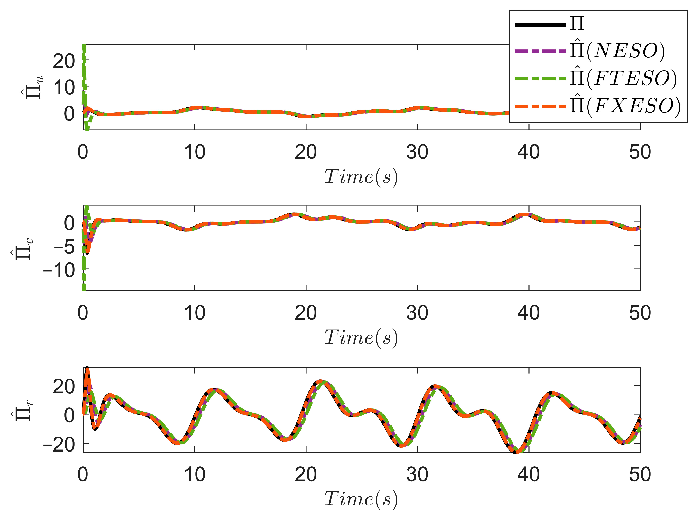
A fixed-time extended state observer is introduced to obtain the estimations of compound perturbations including marine environmental disturbance and unmodeled dynamics.

(2)

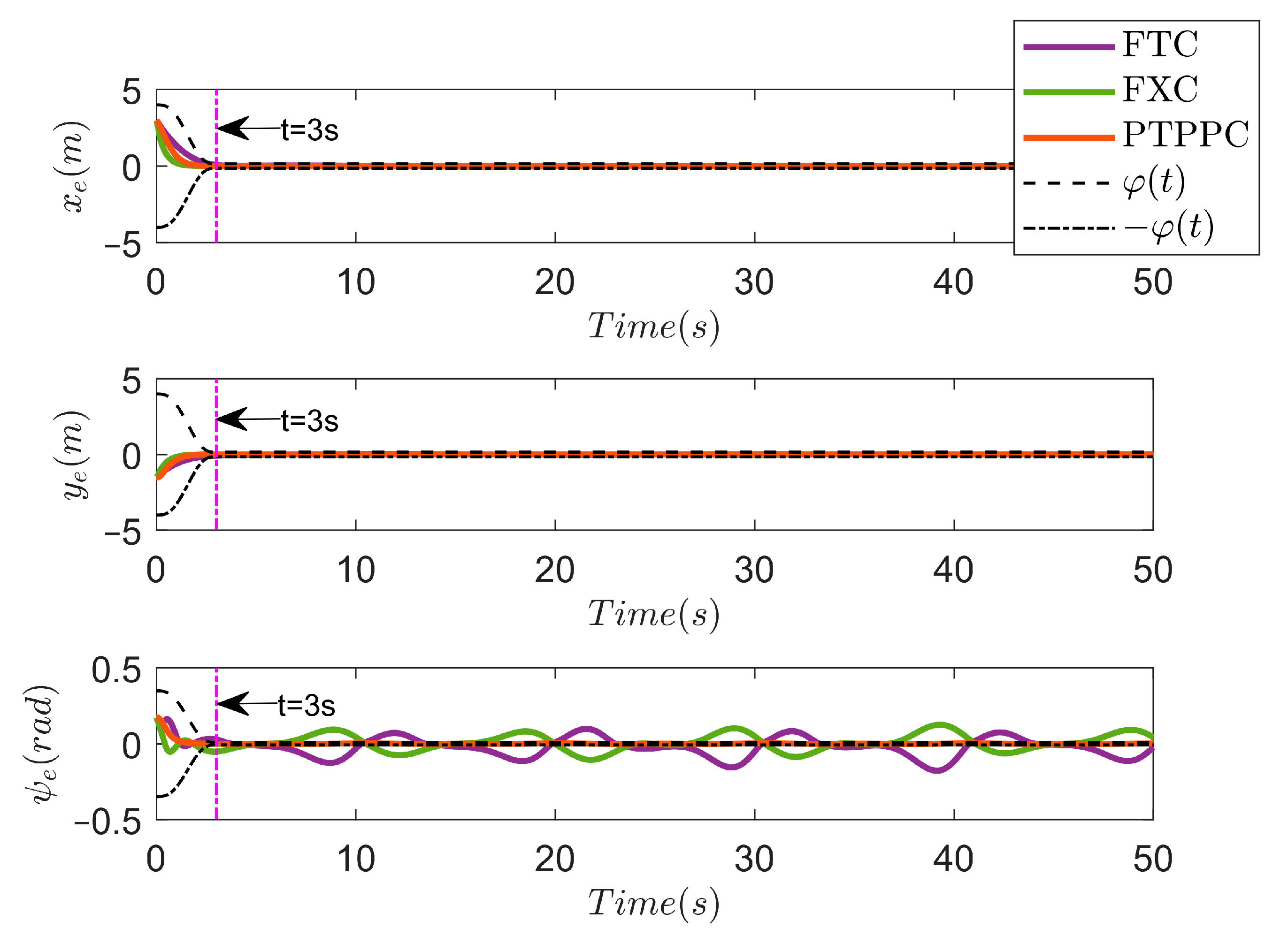
A prescribed-time prescribed performance function is constructed to obtain guaranteed steady-state performance with a prescribed time.

(3)

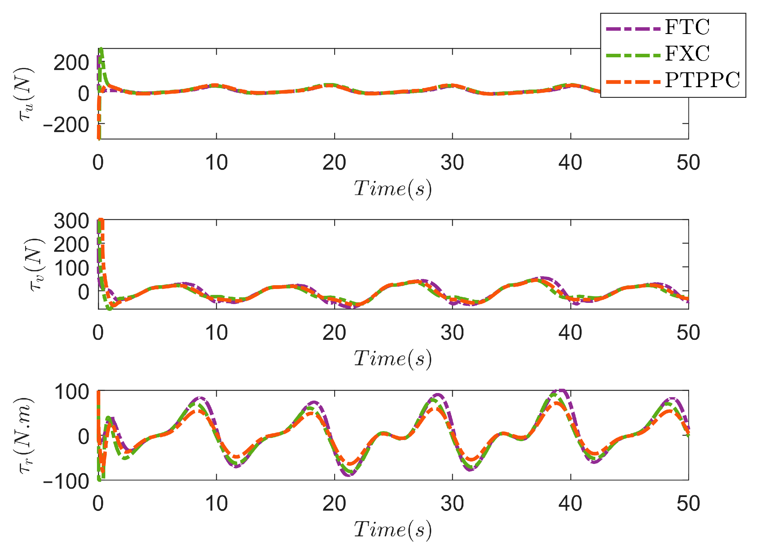
Combining the extended state observer and prescribed performance constraint, a prescribed-time prescribed performance control strategy is presented to ensure the prescribed-time stability of trajectory tracking errors.

The remainder of this article is categorized as follows: Section 2 gives some necessary preliminaries. The main results are displayed in Section 3. Section 4 shows the numerical simulation results, and the conclusion is provided in Section 5.

2. Preliminaries

2.1. Lemma and Assumptions

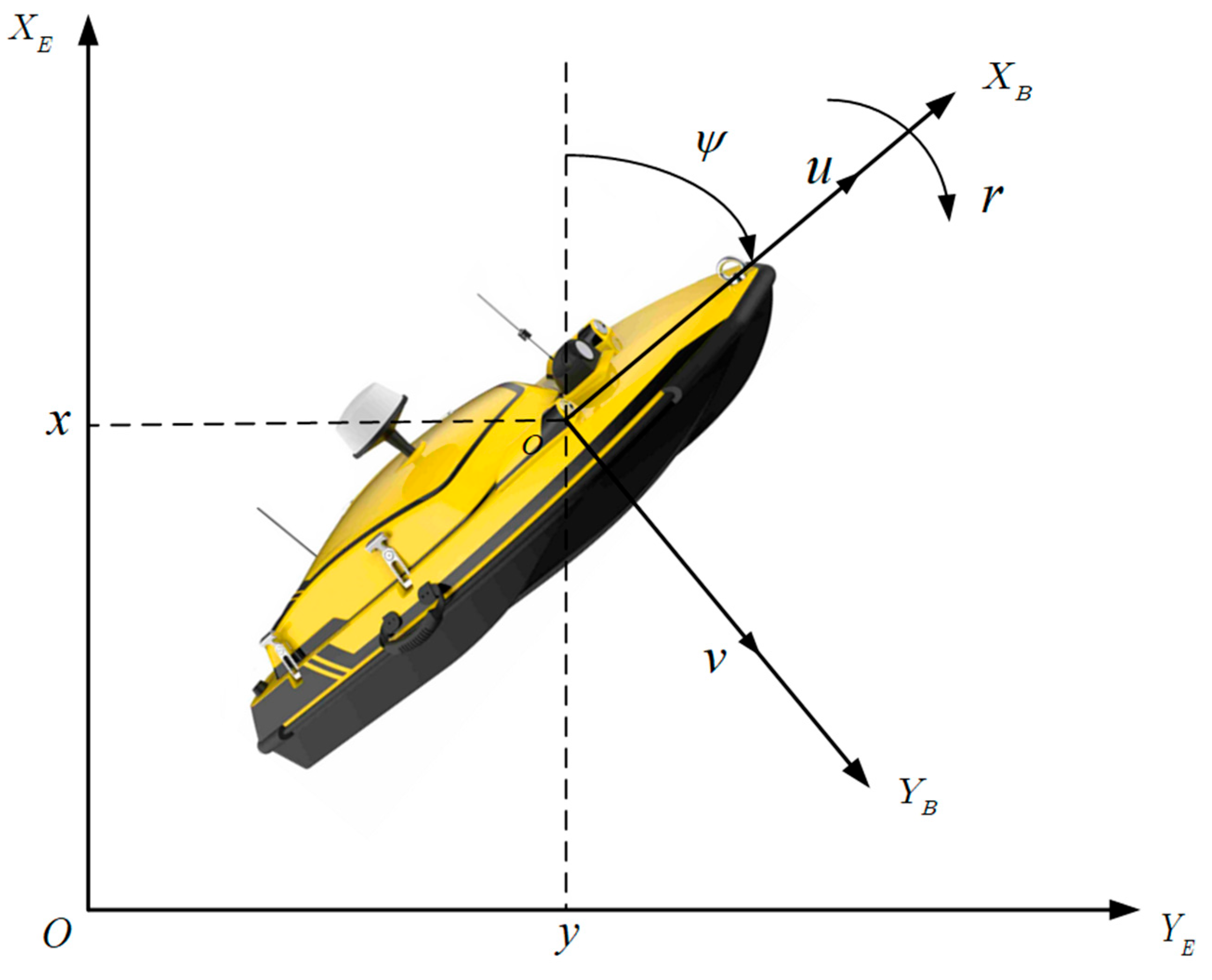
Lemma 1 

[28]. For system $\dot{x}(t)=f(t,x(t)), x(0)=x_0$, if there exists a continuously differentiable function$V(x(t),t)$ satisfies

$$V(0,t)=0, V(x(t),t)>0$$

(1)

$$\dot{V}\le -\mu V+\mathrm{\Pi }$$

(2)

where $\mu >0$ and $\mathrm{\Pi }>0$, then the system is practical prescribed-time stable within the settling time $T$ , and $V(t)$ satisfies $V(t)\equiv 0$ for $t\in [T,\infty )$.

Assumption 1 

[29]. The compound perturbations$\mathrm{\Pi }(\cdot )$, which include marine environmental disturbances and unknown system dynamics, have a bounded rate of change over time; i.e., they satisfy $‖\dot{\mathrm{\Pi }}(\cdot )‖\le D_f$, where $D_f$ denotes a bounded positive constant.

Assumption 2 

[30]. The initial errors satisfy the following predefined constraint:

$$-{\lambda }_1\phi (0)<z(0)<{\lambda }_2\phi (0)$$

(3)

2.2. USV Dynamics

To clearly describe the USV motion model, a body-fixed coordinate system $X_{B}O{Y}_B$ and Earth-fixed coordinate system $X_{E}O{Y}_E$ are established, as shown in Figure 1. On this basis, a three-degree-of-freedom nonlinear USV model is constructed as

$$\left\{\begin{array}{l}\dot{\eta }=J(\psi )\nu \\ M\dot{\nu }+C(\nu )\nu +D(\nu )\nu +g(\nu )={\tau }_p+d\end{array}\right.$$

(4)

where $\eta ={[x,y,\psi ]}^T$ represents the posture vector in the Earth-fixed coordinate system. $\nu ={[u,v,r]}^T$ denotes the velocity vector in the body-fixed coordinate system, where $u$, $v$, and $r$ indicate surge velocity, sway velocity, and yaw angular velocity. $J(\psi )$ is the rotation matrix. $g(\nu )$ denotes the unmodeled dynamics. $d$ represents the marine environmental disturbances. $M$ denotes the inertial matrix. $C(\nu )$ and $D(\nu )$ represent the Coriolis centripetal matrix and the damping matrix, respectively. The detailed expressions of the matrix above can be found in [31]. In practical applications, theoretically calculated control forces and torques are often limited by input saturation.

Therefore, the control law ${\tau }_p$ is designed to consider the thrust and torque under the saturation constraint of the thruster, and its detailed form is given as

$${\tau }_{p,i}=\left\{\begin{array}{ll}sign({\tau }_{c,i}){\tau }_{M,i},& \left|{\tau }_{c,i}\right|\ge {\tau }_{M,i}\\ {\tau }_{ci},& \left|{\tau }_{c,i}\right|<{\tau }_{M,i}\end{array}\right.,i=u,v,r$$

(5)

where ${\tau }_{c,i}$ is the command control input. ${\tau }_{p,i}$ denotes the actual control input. ${\tau }_{Max,i}$ is the maximum force/moment that the actuator can provide at each degree of freedom.

To simplify the later controller design, define ${\varpi }_1=\eta$ and ${\varpi }_2=\dot{\eta }$. Then, (4) is transformed into

$$\left\{\begin{array}{l}{\dot{\varpi }}_1={\varpi }_2\\ {\dot{\varpi }}_2=J(\psi )M^{-1}{\tau }_p+\mathrm{\Pi }(\cdot )\end{array}\right.$$

(6)

where $\mathrm{\Pi }(\cdot )=S(r){\varpi }_2+J(\psi )M^{-1}\left(d-g(v)\right)-J\left(\psi \right)M^{-1}\left(C(\nu )+D(\nu )\right)J{(\psi )}^T{\varpi }_2$ denotes the compound interferences including marine environmental disturbances and model uncertainties. For convenience, $\mathrm{\Pi }(\cdot )$ is replaced by $\mathrm{\Pi }$.

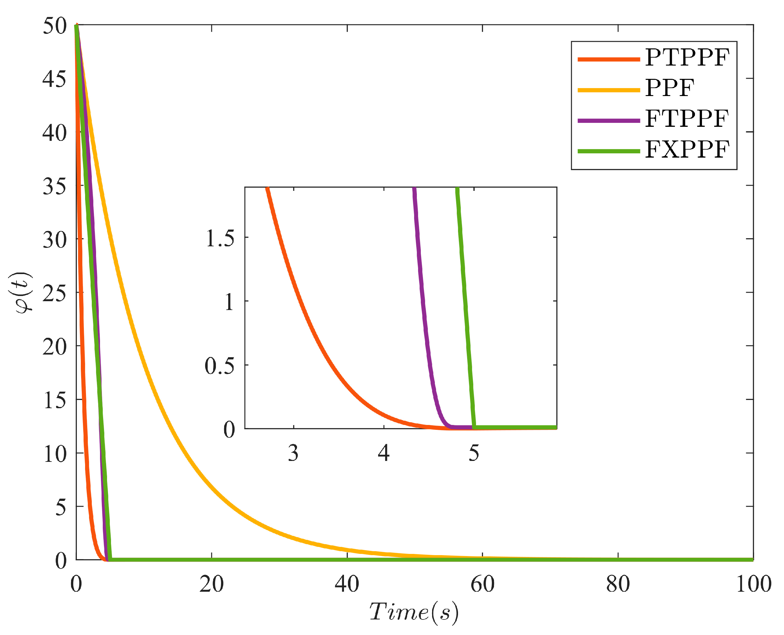
2.3. Prescribed-Time Prescribed Performance Constraint

To obtain guaranteed steady-state performance, and according to (3), the prescribed-time prescribed performance constraint is given as

$$-{\lambda }_1\phi (t)<z(t)<{\lambda }_2\phi (t)$$

(7)

where $z(t)\in R^3$ is the error vector to be designed. ${\lambda }_1$ and ${\lambda }_2$ are designed parameters. $\phi (t)$ represents the boundary constraint that needs to be satisfied.

The mathematical expression for $\dot{\phi }(t)$ has the following definition:

$$\dot{\phi }(t)=-\left({\mathcal{l}}_1+{\mathcal{l}}_2{\displaystyle \frac{{\dot{\gamma }}_{\phi }}{{\gamma }_{\phi }}}\right)\left(\phi (t)-\phi (T_f)\right)+\vartheta$$

(8)

where ${\mathcal{l}}_1>0$ and ${\mathcal{l}}_2>0$ are constants. Furthermore,

$${\gamma }_{\phi }(t)=\left\{\begin{array}{ll}{\displaystyle \frac{T_f^h}{{(T_f+t_0-t)}^h}},& t\in [t_0,T_f)\\ 1,& t\in [T_f,\infty )\end{array}\right.$$

(9)

where the stability time $T_f$ is determined by the user.

Inspired by [32], $\vartheta$ is given as follows:

$$\vartheta =\left\{\begin{array}{ll}({\mathcal{l}}_1+{\mathcal{l}}_2{\displaystyle \frac{{\dot{\gamma }}_{\phi }}{{\gamma }_{\phi }}})(\phi (0)-\phi (T_f))(1-\rho (1-\cos ({\displaystyle \frac{\pi t}{T_m}}))),& t\in [0,T_m)\\ ({\mathcal{l}}_1+{\mathcal{l}}_2{\displaystyle \frac{{\dot{\gamma }}_{\phi }}{{\gamma }_{\phi }}})(\phi (0)-\phi (T_f))({\displaystyle \frac{1}{2}}-\rho )(1+\cos ({\displaystyle \frac{\pi t-\pi T_m}{T_f-T_m}})),& t\in [T_m,T_f)\\ 0,& t\in [T_f,\infty )\end{array}\right.$$

(10)

where $0<T_m<T_f$, $\rho ={\displaystyle \frac{\stackrel{⌣}{\rho }}{\stackrel{⌢}{\rho }}}$, ${\overline{\gamma }}_{\phi }={\mathcal{l}}_1-{\mathcal{l}}_2{\displaystyle \frac{{\dot{\gamma }}_{\phi }}{{\gamma }_{\phi }}}$, $k_{\alpha }={\overline{\gamma }}_{\phi }^2+{({\displaystyle \frac{\pi }{T_m}})}^2$, $k_{\beta }={\overline{\gamma }}_{\phi }^2+{({\displaystyle \frac{\pi }{T_f-T_m}})}^2$.

Moreover, $\stackrel{⌣}{\rho }$ and $\stackrel{⌢}{\rho }$ are designed as follows:

$$\stackrel{⌣}{\rho }=({\displaystyle \frac{1}{2{\overline{\gamma }}_{\phi }}}-{\displaystyle \frac{{\overline{\gamma }}_{\phi }}{2k_{\beta }}})\exp (-{\overline{\gamma }}_{\phi }(T_f-T_m))+{\displaystyle \frac{1}{2{\overline{\gamma }}_{\phi }}}-{\displaystyle \frac{{\overline{\gamma }}_{\phi }}{2k_{\beta }}}$$

(11)

$$\stackrel{⌢}{\rho }=({\displaystyle \frac{{\overline{\gamma }}_{\phi }}{k_{\alpha }}}-{\displaystyle \frac{1}{{\overline{\gamma }}_{\phi }}})\exp (-{\overline{\gamma }}_{\phi }{T}_f)+({\displaystyle \frac{1}{k_{\alpha }}}-{\displaystyle \frac{1}{k_{\beta }}})\exp (-{\overline{\gamma }}_{\phi }(T_f-T_m))+{\displaystyle \frac{1}{{\overline{\gamma }}_{\phi }}}-{\displaystyle \frac{{\overline{\gamma }}_{\phi }}{k_{\beta }}}$$

(12)

The evolution of different prescribed performance functions is displayed in Figure 2. Unlike the traditional prescribed performance function (PPF) [33], finite-time prescribed performance function (FTPPF) [34] and fixed-time prescribed performance function (FXPPF) [35], the suggested PTPPF has a faster convergence rate and can converge to a prescribed constraint within a prescribed time, $T_f$.

3. Main Results

3.1. Design of FXESO

Firstly, to effectively enhance the robustness of the system, a fixed-time extended state observer (FXESO) is introduced to observe the compound perturbations composed of marine environmental disturbance and system uncertainties. The compound perturbations are viewed as an extended state, i.e., $x_3=\mathrm{\Pi }$, and its detailed form is as follows:

$$\left\{\begin{array}{l}{\dot{x}}_1=x_2\\ {\dot{x}}_2=x_3+J(\psi )M^{-1}{\tau }_p\\ {\dot{x}}_3=\hslash \end{array}\right.$$

(13)

where $\hslash$ denotes the first derivative of the extended state.

Subsequently, the fixed-time extended state observer is given as

$$\left\{\begin{array}{l}{\dot{\widehat{x}}}_1={\widehat{x}}_2+m_{1}si{g}^{a_1}({\overline{e}}_1)+n_{1}si{g}^{b_1}({\overline{e}}_1)\\ {\dot{\widehat{x}}}_2={\widehat{x}}_3+m_{2}si{g}^{a_2}({\overline{e}}_1)+n_{2}si{g}^{b_2}({\overline{e}}_1)+J(\psi )M^{-1}{\tau }_p\\ {\dot{\widehat{x}}}_3=m_{3}si{g}^{a_3}({\overline{e}}_1)+n_{3}si{g}^{b_3}({\overline{e}}_1)\end{array}\right.$$

(14)

where ${\widehat{x}}_1$, ${\widehat{x}}_2$, and ${\widehat{x}}_3$ are the estimations of $x_1$, $x_2$, and $x_3$, respectively.$a\in \left(2/3,1\right)$ and $a_i=i(a-1)+1$; $b=1/a$ and $b_i=b+(i-1)\left(1/b-1\right),i=1,2,3$. The appropriate matrix is selected, namely,

$$W_1=\left[\begin{array}{ccc}-m_1& 1& 0\\ -m_2& 0& 1\\ -m_3& 0& 0\end{array}\right],W_2=\left[\begin{array}{ccc}-n_1& 1& 0\\ -n_2& 0& 1\\ -n_3& 0& 0\end{array}\right]$$

(15)

where $W_1$ and $W_2$ are Hurwitz.

Theorem 1 

.Considering system (6) under Assumption 1, the observer takes the form (14) and selects the appropriate parameters m_i, n_i, a_i, and b_i, and the observation errors ${\overline{e}}_1$, ${\overline{e}}_2$, and ${\overline{e}}_3$ will converge to equilibrium point within a fixed time.

Proof of Theorem 1. 

Define the following error vector:

$$\left\{\begin{array}{l}{\overline{e}}_1=x_1-{\widehat{x}}_1\\ {\overline{e}}_2=x_2-{\widehat{x}}_2\\ {\overline{e}}_3=x_3-{\widehat{x}}_3\end{array}\right.$$

(16)

Combining (13) and (14), the following observation error dynamics can be obtained:

$$\left\{\begin{array}{l}{\dot{\overline{e}}}_1={\overline{e}}_2-m_{1}si{g}^{a_1}{\overline{e}}_1-n_{1}si{g}^{b_1}{\overline{e}}_1\\ {\dot{\overline{e}}}_2={\overline{e}}_3-m_{2}si{g}^{a_2}{\overline{e}}_1-n_{2}si{g}^{b_2}{\overline{e}}_1\\ {\dot{\overline{e}}}_3=\hslash -m_{3}si{g}^{a_3}{\overline{e}}_1-n_{3}si{g}^{b_3}{\overline{e}}_1\end{array}\right.$$

(17)

After transformation, the designed fixed-time state observer is the same as the state observer proposed in [29], and the observation error can quickly approach to the equilibrium point within the fixed time $T_o\le {\displaystyle \frac{1}{{\mu }_1(1-d_m)}}+{\displaystyle \frac{1}{{\mu }_2(d_n-1)}}$. The detailed parameters and derivation process can be founded in [29]. $\square$

3.2. Controller Design

Firstly, define the following trajectory tracking error:

$$e=\eta -{\eta }_d$$

(18)

where ${\eta }_d$ represents the reference trajectory. $e={[x_e,y_e,{\psi }_e]}^T$, $x_e=x-x_d$, $y_e=y-y_d$, ${\psi }_e=\psi -{\psi }_d$. Subsequently, the following auxiliary error vector is designed:

$$z_i=(k_e+c_e{\displaystyle \frac{\dot{\gamma }}{\gamma }})e_i ,i=1,2,3$$

(19)

where $k_e>0$ and $c_e>0$. Differentiating ${\dot{z}}_i$, we obtain

$${\dot{z}}_i={\displaystyle \frac{c_e(\gamma \ddot{\gamma }-{\dot{\gamma }}^2)}{{\gamma }^2}}{e}_i+(k_e+c_e{\displaystyle \frac{\dot{\gamma }}{\gamma }}){\dot{e}}_i, i=1,2,3$$

(20)

Due to the difficulty in directly designing the controller under constraint (7), the following error transformation is introduced:

$$z_i={\lambda }_2\phi (t)\mathrm{\gamma }(s_{1i},\mathrm{ƛ})$$

(21)

where $\mathrm{ƛ}={\displaystyle \frac{{\lambda }_1}{{\lambda }_2}}$ and $\mathrm{\gamma }(s_1,\mathrm{ƛ})={\displaystyle \frac{e^{s_1}-e^{-s_1}}{e^{s_1}+{\mathrm{ƛ}}^{-1}{e}^{-s_1}}}$ increases monotonically.

Thus, the transformation error $s_{1i}$ is obtained by solving (21).

$$s_{1i}={\displaystyle \frac{1}{2}}\ln \left({\displaystyle \frac{{\lambda }_1{\lambda }_2\phi +{\lambda }_2{z}_i}{{\lambda }_1{\lambda }_2\phi -{\lambda }_1{z}_i}}\right)$$

(22)

Subsequently, taking the time derivative of $s_{1i}$ yields

$${\dot{s}}_{1i}={\partial }_i({\dot{z}}_i-z_i\dot{\phi }{\phi }^{-1})$$

(23)

where ${\partial }_i=\left({\displaystyle \frac{1}{2(z_i+{\lambda }_1\phi )}}-{\displaystyle \frac{1}{2(z_i-{\lambda }_2\phi )}}\right)$.

The subsequent Lyapunov function is established as

$$V_1={\displaystyle \frac{1}{2}}{s}_1^T{s}_1$$

(24)

The time derivative of $V_1$, along with (22), is

$$\begin{array}{cc}\hfill {\dot{V}}_1& =s_1^T\left(\partial (\dot{z}-z\dot{\phi }{\phi }^{-1})\right)\hfill \\ & =s_1^T\left(\partial \left({\displaystyle \frac{c_e(\gamma \ddot{\gamma }-{\dot{\gamma }}^2)}{{\gamma }^2}}e+(k_e+c_e{\displaystyle \frac{\dot{\gamma }}{\gamma }})(\xi -{\dot{\eta }}_d)-z\dot{\phi }{\phi }^{-1}\right)\right)\hfill \end{array}$$

(25)

Given that $\mathit{\nu }$ represents the virtual control signal, we develop the following virtual control law:

$$\alpha ={\left(k_e+c_e{\displaystyle \frac{\dot{\gamma }}{\gamma }}\right)}^{-1}\left[z\dot{\phi }{\phi }^{-1}-{\partial }^{-1}{\kappa }_1{s}_1-{\displaystyle \frac{c_e(\gamma \ddot{\gamma }-{\dot{\gamma }}^2)}{{\gamma }^2}}e\right]+{\dot{\eta }}_d$$

(26)

where ${\kappa }_1$ denotes a positive constant.

Subsequently, the velocity tracking error is given in conjunction with the dynamic surface control technique:

$$s_2=\xi -{\alpha }_f$$

(27)

$$\varphi ={\alpha }_f-\alpha$$

(28)

where $\varphi$ is the filtering error, and ${\alpha }_f$ indicates the filter output.

$$\iota {\dot{\alpha }}_f+{\alpha }_f=\alpha , {\alpha }_f(0)=\alpha (0)$$

(29)

where $\iota$ is the filter time constant.

From (28) and (29), we have

$$\dot{\varphi }=-{\displaystyle \frac{1}{\iota }}\varphi +\Delta$$

(30)

where $\Delta =-\dot{\alpha }$.

By differentiating $s_2$ with respect to time and applying (5) and (27), we derive the following expression:

$$\begin{array}{ll}{\dot{s}}_2& =J(\psi )M^{-1}{\tau }_p+\mathrm{\Pi }-{\dot{\alpha }}_f\\ & =J(\psi )M^{-1}({\tau }_c+\Delta \tau )+\mathrm{\Pi }-{\dot{\alpha }}_f\end{array}$$

(31)

To mitigate the term $\Delta \tau$ caused by (31), we implement the linear anti-windup compensator as follows:

$$\dot{\mathrm{\Xi }}=-K_{\mathrm{\Xi }}\mathrm{\Xi }+\Delta \tau$$

(32)

where $K_{\mathrm{\Xi }}$ denotes a positive designed matrix, and $\mathrm{\Xi }\in R^3$ denotes state vector of compensator.

Then, the prescribed-time controller with PTPPF constraint is designed as follows:

$${\tau }_p=MJ{(\psi )}^T\left(-{\kappa }_2{s}_2+{\dot{\alpha }}_f-\widehat{\mathrm{\Pi }}\right)+{\kappa }_3\mathrm{\Xi }$$

(33)

where ${\kappa }_2>0$ and $\widehat{\mathrm{\Pi }}$ is the estimated value of $\mathrm{\Pi }$.

Theorem 2.

Consider system (6), combined with the FXESO (14), the kinematic controller (26), and the dynamic controller (33), the trajectory tracking error e will converge to the equilibrium point within the prescribed time T.

Proof of Theorem 2.

Construct the following Lyapunov function:

$$V={\displaystyle \frac{1}{2}}{s}_1^T{s}_1+{\displaystyle \frac{1}{2}}{s}_2^T{s}_2+{\displaystyle \frac{1}{2}}{\mathrm{\Xi }}^T\mathrm{\Xi }+{\displaystyle \frac{1}{2}}{\varphi }^T\varphi$$

(34)

Differentiating (34), it yields

$$\dot{V}=s_1^T{\dot{s}}_1+s_2^T{\dot{s}}_2+{\mathrm{\Xi }}^T\dot{\mathrm{\Xi }}+{\varphi }^T\dot{\varphi }$$

(35)

It follows from (27) and (28) that $\xi =s_2+\varphi +\alpha$. Then, combining (23), we have

$$\begin{array}{ll}{s}_1^T{\dot{s}}_1& =s_1^T\left(\partial (\dot{z}-z\dot{\phi }{\phi }^{-1})\right)\\ & =s_1^T\left(\partial \left({\displaystyle \frac{c_e(\gamma \ddot{\gamma }-{\dot{\gamma }}^2)}{{\gamma }^2}}e+(k_e+c_e{\displaystyle \frac{\dot{\gamma }}{\gamma }})(\xi -{\dot{\eta }}_d)-z\dot{\phi }{\phi }^{-1}\right)\right)\\ & =s_1^T\left(\partial \left({\displaystyle \frac{c_e(\gamma \ddot{\gamma }-{\dot{\gamma }}^2)}{{\gamma }^2}}e+(k_e+c_e{\displaystyle \frac{\dot{\gamma }}{\gamma }})(s_2+\varphi +\alpha -{\dot{\eta }}_d)-z\dot{\phi }{\phi }^{-1}\right)\right)\end{array}$$

(36)

Substituting (23) into (36) yields

$$\begin{array}{ll}{s}_1^T{\dot{s}}_1& =s_1^T\left(\partial \left(k_e+c_e{\displaystyle \frac{\dot{\gamma }}{\gamma }}\right)\left(s_2+\varphi \right)-{\kappa }_1{s}_1\right)\\ & =\partial \left(k_e+c_e{\displaystyle \frac{\dot{\gamma }}{\gamma }}\right)s_1^T{s}_2+\partial \left(k_e+c_e{\displaystyle \frac{\dot{\gamma }}{\gamma }}\right)s_1^T\varphi -{\kappa }_1{s}_1^T{s}_1\end{array}$$

(37)

By using Young’s inequality, we obtain

$$\begin{array}{l}{s}_1^T{\dot{s}}_1=\partial \left(k_e+c_e{\displaystyle \frac{\dot{\gamma }}{\gamma }}\right)s_1^T{s}_2+\partial \left(k_e+c_e{\displaystyle \frac{\dot{\gamma }}{\gamma }}\right)s_1^T\varphi -{\kappa }_1{s}_1^T{s}_1\\ \le \partial \left(k_e+c_e{\displaystyle \frac{\dot{\gamma }}{\gamma }}\right)({\displaystyle \frac{1}{2}}{s}_1^T{s}_1+{\displaystyle \frac{1}{2}}{s}_2^T{s}_2)+\partial \left(k_e+c_e{\displaystyle \frac{\dot{\gamma }}{\gamma }}\right)({\displaystyle \frac{1}{2}}{s}_1^T{s}_1+{\displaystyle \frac{1}{2}}{\varphi }^T\varphi )-{\kappa }_1{s}_1^T{s}_1\\ \le -\left[{\kappa }_1-\partial \left(k_e+c_e{\displaystyle \frac{\dot{\gamma }}{\gamma }}\right)\right]s_1^T{s}_1+{\displaystyle \frac{1}{2}}\partial \left(k_e+c_e{\displaystyle \frac{\dot{\gamma }}{\gamma }}\right)s_2^T{s}_2+{\displaystyle \frac{1}{2}}\partial \left(k_e+c_e{\displaystyle \frac{\dot{\gamma }}{\gamma }}\right){\varphi }^T\varphi \end{array}$$

(38)

From (28) and (30), we have

$${\varphi }^T\dot{\varphi }={\varphi }^T\left(-{\displaystyle \frac{1}{\iota }}\varphi +\Delta \right)$$

(39)

$${\mathrm{\Xi }}^T\dot{\mathrm{\Xi }}={\mathrm{\Xi }}^T\left(-K_{\mathrm{\Xi }}\mathrm{\Xi }+\Delta \tau \right)$$

(40)

Subsequently, in light of (38)–(40), (35) can be further written as

$$\begin{array}{ll}\dot{V}\le & -\left[{\kappa }_1-\partial \left(k_e+c_e{\displaystyle \frac{\dot{\gamma }}{\gamma }}\right)\right]s_1^T{s}_1+{\displaystyle \frac{1}{2}}\partial \left(k_e+c_e{\displaystyle \frac{\dot{\gamma }}{\gamma }}\right)s_2^T{s}_2+{\displaystyle \frac{1}{2}}\partial \left(k_e+c_e{\displaystyle \frac{\dot{\gamma }}{\gamma }}\right){\varphi }^T\varphi \\ & -{\displaystyle \frac{1}{\iota }}{\varphi }^T\varphi +{\varphi }^T\Delta -{\mathrm{\Xi }}^T{K}_{\mathrm{\Xi }}\mathrm{\Xi }+{\mathrm{\Xi }}^T\Delta \tau -{\kappa }_2{s}_2^T{s}_2\end{array}$$

(41)

Consider the compact set ${\mathrm{\Omega }}_d=\left\{{\left[{\eta }_d^T,{\dot{\eta }}_d^T,{\ddot{\eta }}_d^T\right]}^T:{‖{\eta }_d‖}^2+{‖{\dot{\eta }}_d‖}^2+{‖{\ddot{\eta }}_d‖}^2\le B_0,B_0>0\right\}$ and ${\mathrm{\Omega }}_1=\left\{{\left[s_1^T,s_2^T,{\varphi }^T\right]}^T:V\le {\hslash }_0,{\hslash }_0>0\right\}$, and ${\mathrm{\Omega }}_d\times {\mathrm{\Omega }}_1$ is also a compact set. Then, there exists a non-negative continuous function $\beta (\cdot )$ such that $‖\Delta ‖\le \beta (\cdot )$ and $\beta (\cdot )$ has maximum $N$ on ${\mathrm{\Omega }}_d\times {\mathrm{\Omega }}_1$ [36].

The following inequality holds in accordance with Young’s inequality:

$${\varphi }^T\Delta \le a_1{\varphi }^T\varphi +{\displaystyle \frac{N^2}{4a_1}}$$

(42)

Substituting (42) into (41) yields

$$\begin{array}{l}\dot{V}\le -\left[{\kappa }_1-\partial \left(k_e+c_e{\displaystyle \frac{\dot{\gamma }}{\gamma }}\right)\right]s_1^T{s}_1-\left[{\kappa }_2-{\displaystyle \frac{1}{2}}\partial \left(k_e+c_e{\displaystyle \frac{\dot{\gamma }}{\gamma }}\right)\right]s_2^T{s}_2\\ +{\displaystyle \frac{1}{2}}\partial \left(k_e+c_e{\displaystyle \frac{\dot{\gamma }}{\gamma }}\right){\varphi }^T\varphi -{\displaystyle \frac{1}{\iota }}{\varphi }^T\varphi +a_1{\varphi }^T\varphi +{\displaystyle \frac{N^2}{4a_1}}-{\mathrm{\Xi }}^T{K}_{\mathrm{\Xi }}\mathrm{\Xi }+{\mathrm{\Xi }}^T\Delta \tau \end{array}$$

(43)

Let $k_{\mathrm{\Xi }}={\lambda }_{\min }(K_{\mathrm{\Xi }})$. Combined with Young’s inequality, we obtain

$$\begin{array}{l}\dot{V}\le -\left[{\kappa }_1-\partial \left(k_e+c_e{\displaystyle \frac{\dot{\gamma }}{\gamma }}\right)\right]s_1^T{s}_1-\left[{\kappa }_2-{\displaystyle \frac{1}{2}}\partial \left(k_e+c_e{\displaystyle \frac{\dot{\gamma }}{\gamma }}\right)\right]s_2^T{s}_2\\ -\left[{\displaystyle \frac{1}{\iota }}-{\displaystyle \frac{1}{2}}\partial -a_1\left(k_e+c_e{\displaystyle \frac{\dot{\gamma }}{\gamma }}\right)\right]{\varphi }^T\varphi -\left(k_{\mathrm{\Xi }}-{\displaystyle \frac{1}{2}}\right){‖\mathrm{\Xi }‖}^2+{\displaystyle \frac{1}{2}}{‖\Delta \tau ‖}^2+{\displaystyle \frac{N^2}{4a_1}}\end{array}$$

(44)

Select appropriate parameters such that ${\mathrm{\Lambda }}_1={\kappa }_1-\partial \left(k_e+c_e{\displaystyle \frac{\dot{\gamma }}{\gamma }}\right)>0$, ${\mathrm{\Lambda }}_2={\kappa }_2-{\displaystyle \frac{1}{2}}\partial \left(k_e+c_e{\displaystyle \frac{\dot{\gamma }}{\gamma }}\right)>0$, ${\mathrm{\Lambda }}_3={\displaystyle \frac{1}{\iota }}-{\displaystyle \frac{1}{2}}\partial -a_1\left(k_e+c_e{\displaystyle \frac{\dot{\gamma }}{\gamma }}\right)>0$ and ${\mathrm{\Lambda }}_4=k_{\mathrm{\Xi }}-{\displaystyle \frac{1}{2}}>0$.

Then, we have

$$\dot{V}\le -2\varsigma V+\mathrm{\Pi }$$

(45)

where $\varsigma =\min \left\{{\mathrm{\Lambda }}_1,{\mathrm{\Lambda }}_2,{\mathrm{\Lambda }}_3,{\mathrm{\Lambda }}_4\right\}$ and $\mathrm{\Pi }={\displaystyle \frac{1}{2}}{‖\Delta \tau ‖}^2+{\displaystyle \frac{N^2}{4a_1}}$. According to Lemma 1, it is obvious that $V$ can be stable at the prescribed time $T$. Hence, the prescribed-time convergence of all signals of the system can be guaranteed. This completes the proof. $\square$

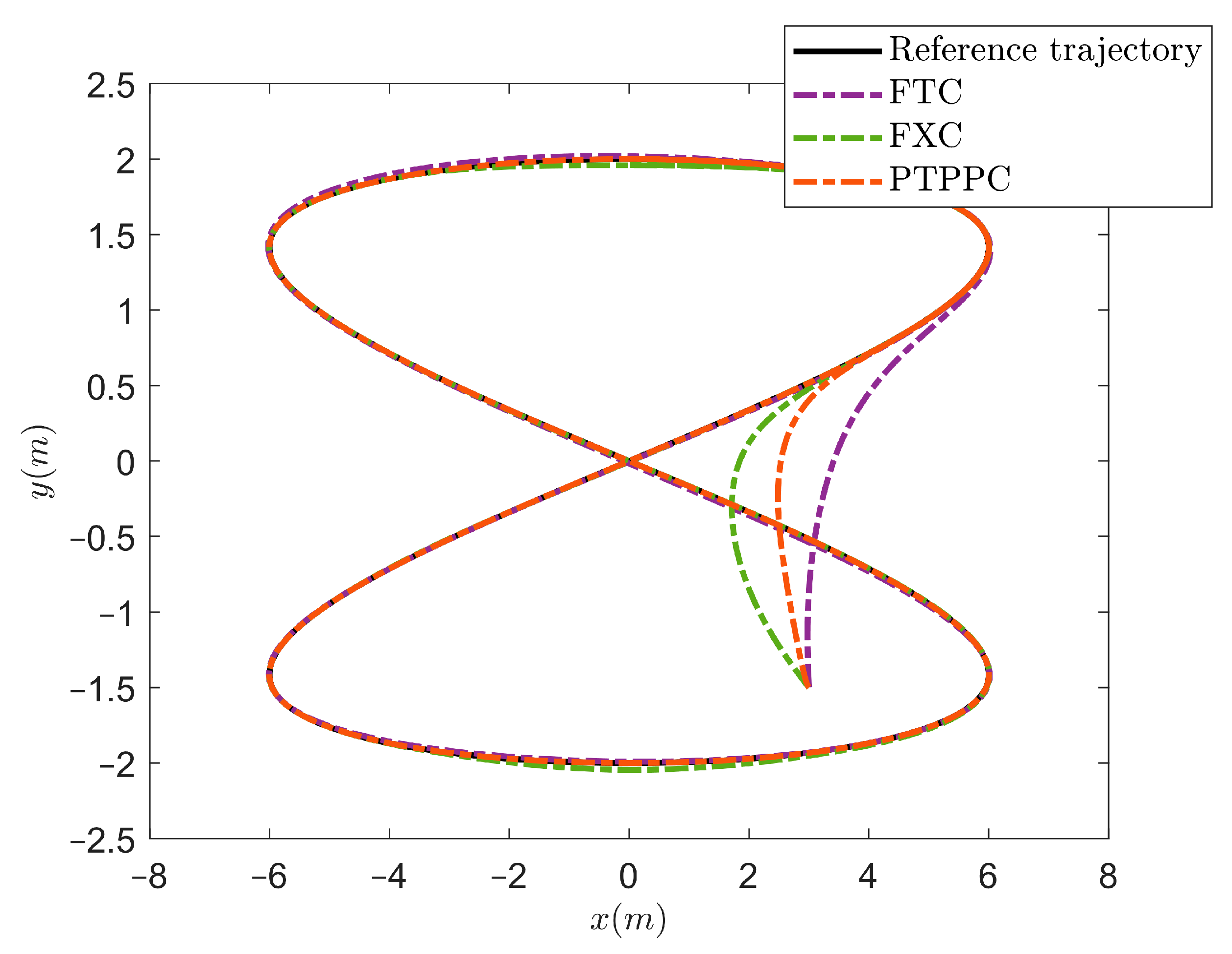
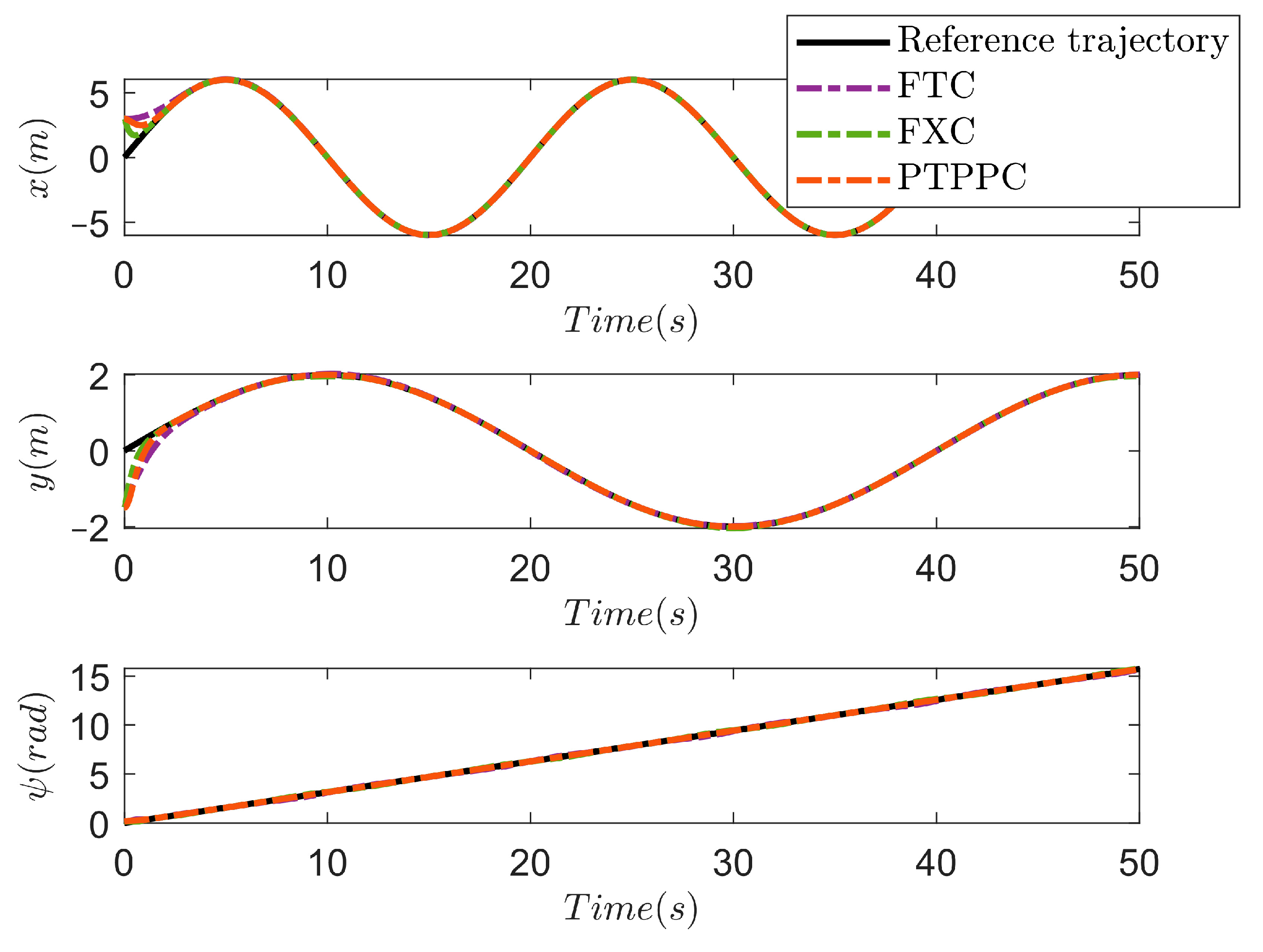
4. Simulation Results

To demonstrate the superiority of the presented control algorithm, this research employs the classical Cybership II model for simulation verification. And its detailed hydrodynamic parameters are referenced in [37]. For reflecting the advantage of the proposed prescribed-time prescribed performance control (PTPPC) strategy in this article, the finite-time control (FTC) scheme in [38] and the fixed-time control (FXC) scheme in [39] are used for comparative experiments. In addition, the nonlinear extended state observer (NESO) in [40] and the finite-time extended state observer (FTESO) in [29] are used for comparison with the proposed FXESO in this paper. The reference trajectory is chosen as ${\eta }_d={[6\sin (0.1\pi t),2\sin (0.05\pi t),0.1\pi t]}^T$. The parameters of the PTPPF are given as ${\lambda }_1={\lambda }_2=1$, $\phi (0)={[4,4,\pi /9]}^T$, $\phi (T_f)={[0.15,0.15,\pi /360]}^T$, $T_f=3 \mathrm{s}$. The initial conditions of USV are chosen as $\eta (0)={[3,-1.5,\pi /18]}^T$, $\nu (0)={[0,0,0]}^T$. The maximum and minimum values of the saturation constraint are ${[300,300,100]}^T$ and ${[-300,-300,-100]}^T$. The marine environmental interferences and unmodeled dynamics are set to $d={[3\sin (0.4t),2\sin (0.2t),1.5\sin (0.3t)]}^T$, $g(\nu )={[0.3u{v}^2,0.1uv,0.2u{r}^2]}^T$. The settling time $T=T_f=3 \mathrm{s}$. The parameters of the FXESO and the PTPPC are given in

Table 1. The parameters of FXESO and PTPPC.

Parameter	Value	Parameter	Value
$m_1$	5	$a_2$	0.6
$m_2$	15	$a_3$	0.4
$m_3$	35	$b_1$	1.25
$n_1$	15	$b_2$	1.05
$n_2$	40	$b_3$	0.85
$n_3$	55	${\kappa }_2$	$diag(50,50,100)$
$a_1$	0.8	${\kappa }_3$	$diag(0.1,0.1,0.1)$

.

The simulation results are displayed in Figure 3, Figure 4, Figure 5, Figure 6 and Figure 7. Figure 3 illustrates the tracking trajectory of USVs under three control schemes. From Figure 3, although the three control schemes can track the reference trajectory, the PTPPC control strategy suggested in this paper can converge to the desired trajectory more quickly and accurately. The user can preset the convergence time of the PTPPC strategy in advance. Figure 4 shows the evolution curves of position and heading angle under the action of three controllers. Subsequently, the trajectory tracking errors under three control schemes are displayed in Figure 5. As shown in Figure 5, considering complex disturbances, unknown system dynamics, and thruster saturation, the posture tracking error under the presented PTPPC strategy converges more rapidly and accurately to the preset performance constraints within the prescribed time $T=3 \mathrm{s}$ and is strictly maintained within the specified constraint range. Although the FXC control strategy appears to have a faster convergence trend in the early stage, it tends to require more extensive control input, resulting in greater energy consumption. In addition, we can find that the tracking accuracy of the PTPPC scheme is better than that of the FXC control scheme. On one hand, the FTC control algorithm has the slowest convergence rate. On the other hand, neither the FXC control algorithm nor the FTC control scheme can converge to the predefined performance constraints within a preset time. Figure 6 illustrates the observation values of compound perturbations under three types of extended state observers. According to Figure 6, in the initial stage, the estimation result of FTESO has a significant overshoot, which will weaken the robustness of the controller. Compared with the NESO and the FTESO, the introduced FXESO can quickly and accurately observe the compound disturbances and improve the robustness of controller. Figure 7 depicts the control input curves of three controllers. For the sake of fairness, the same saturation suppression has been applied to all three controllers in this paper. Obviously, under the action of a linear compensator, the effect of thruster saturation on control quality is effectively alleviated. Furthermore, the integral absolute error (IAE) is given in

Table 2. IAE of the three control strategies.

Indices	Errors	PTPPC	FXC	FTC
$IAE={\displaystyle {\int }_0^T\left|e(t)\right|}dt$	$x_e$	2.058	1.849	3.724
	$y_e$	1.094	1.147	1.936
	${\psi }_e$	0.146	2.094	2.640

to quantify the tracking performance of the three controllers, which clearly display the superiority of the proposed controller.

5. Conclusions

This paper presents a prescribed-time prescribed performance control strategy for the USV trajectory tracking control problem with compound interferences. The introduced fixed-time extended state observer can quickly observe compound perturbations within a fixed time and mitigate the influence of compound disturbances on control performance. Then, a novel prescribed-time prescribed performance constraint is designed to ensure that the trajectory tracking error converges to the predefined constraint boundary within the prescribed time. In addition, a linear compensator is introduced to alleviate input saturation. The prescribed-time convergence performance of the system is proved by constructing the Lyapunov function. Finally, multiple simulation comparison tests validate that the proposed control scheme can achieve better estimation performance, faster transient response, and higher tracking accuracy. In future work, the issue of USV prescribed-time formation tracking control will be investigated.

References

1. Jin, J.; Liu, D.; Wang, D.; Ma, Y. A practical trajectory tracking scheme for a twin-propeller twin-hull unmanned surface vehicle. J. Mar. Sci. Eng. 2021, 9, 1070. [Google Scholar] [CrossRef]
2. Park, B.S.; Kwon, J.W.; Kim, H. Neural network-based output feedback control for reference tracking of underactuated surface vessels. Automatica 2017, 77, 353–359. [Google Scholar] [CrossRef]
3. Gao, S.; Peng, Z.; Liu, L.; Wang, D.; Han, Q.-L. Fixed-time resilient edge-triggered estimation and control of surface vehicles for cooperative target tracking under attacks. IEEE Trans. Intell. Veh. 2022, 8, 547–556. [Google Scholar] [CrossRef]
4. Song, X.; Wu, C.; Stojanovic, V.; Song, S. 1 bit encoding–decoding-based event-triggered fixed-time adaptive control for unmanned surface vehicle with guaranteed tracking performance. Control Eng. Pract. 2023, 135, 105513. [Google Scholar] [CrossRef]
5. Liao, Y.; Zhang, M.; Wan, L.; Li, Y. Trajectory tracking control for underactuated unmanned surface vehicles with dynamic uncertainties. J. Cent. South Univ. 2016, 23, 370–378. [Google Scholar] [CrossRef]
6. Dong, Z.; Wan, L.; Li, Y.; Liu, T.; Zhang, G. Trajectory tracking control of underactuated USV based on modified backstepping approach. Int. J. Nav. Archit. Ocean Eng. 2015, 7, 817–832. [Google Scholar] [CrossRef]
7. Liu, W.; Ye, H.; Yang, X. Super-twisting sliding mode control for the trajectory tracking of underactuated USVs with disturbances. J. Mar. Sci. Eng. 2023, 11, 636. [Google Scholar] [CrossRef]
8. Lei, T.; Wen, Y.; Yu, Y.; Tian, K.; Zhu, M. Predictive trajectory tracking control for the USV in networked environments with communication constraints. Ocean Eng. 2024, 298, 117185. [Google Scholar] [CrossRef]
9. Qin, J.; Du, J. Robust adaptive asymptotic trajectory tracking control for underactuated surface vessels subject to unknown dynamics and input saturation. J. Mar. Sci. Technol. 2022, 27, 307–319. [Google Scholar] [CrossRef]
10. Qin, H.; Li, C.; Sun, Y. Adaptive neural network-based fault-tolerant trajectory-tracking control of unmanned surface vessels with input saturation and error constraints. IET Intell. Transp. Syst. 2020, 14, 356–363. [Google Scholar] [CrossRef]
11. Luo, Q.; Wang, H.; Li, N.; Su, B.; Zheng, W. Model-free predictive trajectory tracking control and obstacle avoidance for unmanned surface vehicle with uncertainty and unknown disturbances via model-free extended state observer. Int. J. Control Autom. Syst. 2024, 22, 1985–1997. [Google Scholar] [CrossRef]
12. Zheng, H.; Li, J.; Tian, Z.; Liu, C.; Wu, W. Hybrid physics-learning model based predictive control for trajectory tracking of unmanned surface vehicles. IEEE Trans. Intell. Transp. Syst. 2024. [Google Scholar] [CrossRef]
13. Qiu, B.; Wang, G.; Fan, Y.; Mu, D.; Sun, X. Adaptive sliding mode trajectory tracking control for unmanned surface vehicle with modeling uncertainties and input saturation. Appl. Sci. 2019, 9, 1240. [Google Scholar] [CrossRef]
14. Yan, Z.; Wang, M.; Xu, J. Robust adaptive sliding mode control of underactuated autonomous underwater vehicles with uncertain dynamics. Ocean Eng. 2019, 173, 802–809. [Google Scholar] [CrossRef]
15. Mu, D.; Wang, G.; Fan, Y.; Qiu, B.; Sun, X. Adaptive course control based on trajectory linearization control for unmanned surface vehicle with unmodeled dynamics and input saturation. Neurocomputing 2019, 330, 1–10. [Google Scholar] [CrossRef]
16. Esfahani, H.N.; Szlapczynski, R. Model predictive super-twisting sliding mode control for an autonomous surface vehicle. Pol. Marit. Res. 2019, 26, 163–171. [Google Scholar] [CrossRef]
17. Wang, N.; Gao, Y.; Yang, C.; Zhang, X. Reinforcement learning-based finite-time tracking control of an unknown unmanned surface vehicle with input constraints. Neurocomputing 2022, 484, 26–37. [Google Scholar] [CrossRef]
18. Xu, D.; Liu, Z.; Song, J.; Zhou, X. Finite time trajectory tracking with full-state feedback of underactuated unmanned surface vessel based on nonsingular fast terminal sliding mode. J. Mar. Sci. Eng. 2022, 10, 1845. [Google Scholar] [CrossRef]
19. Chen, H.; Zhang, D.; Zhao, M.; Xie, S. Finite-time tracking control of underactuated surface vehicle with tracking error constraints. Int. J. Veh. Des. 2020, 1, 84. [Google Scholar] [CrossRef]
20. Zhang, L.; Zheng, Y.; Huang, B.; Su, Y. Finite-time trajectory tracking control for under-actuated unmanned surface vessels with saturation constraint. Ocean Eng. 2022, 249, 110745. [Google Scholar] [CrossRef]
21. Chen, Q.; Zhao, Y.; Wen, G.; Shi, G.; Yu, X. Fixed-time cooperative tracking control for double-integrator multiagent systems: A time-based generator approach. IEEE Trans. Cybern. 2022, 53, 5970–5983. [Google Scholar] [CrossRef] [PubMed]
22. Zou, Q.; Chang, S. A new fixed-time terminal sliding mode control for second-order nonlinear systems. J. Frankl. Inst. 2024, 361, 1255–1267. [Google Scholar] [CrossRef]
23. Yao, Q. Fixed-time trajectory tracking control for unmanned surface vessels in the presence of model uncertainties and external disturbances. Int. J. Control 2022, 95, 1133–1143. [Google Scholar] [CrossRef]
24. Sui, B.; Zhang, J.; Liu, Z.; Wei, J. Fixed-Time Trajectory Tracking Control of Fully Actuated Unmanned Surface Vessels with Error Constraints. J. Mar. Sci. Eng. 2024, 12, 584. [Google Scholar] [CrossRef]
25. Song, Y.; Wang, Y.; Holloway, J.; Krstic, M. Time-varying feedback for regulation of normal-form nonlinear systems in prescribed finite time. Automatica 2017, 83, 243–251. [Google Scholar] [CrossRef]
26. Li, Y.; He, J.; Shen, H.; Zhang, W.; Li, Y. Adaptive practical prescribed-time fault-tolerant control for autonomous underwater vehicles trajectory tracking. Ocean Eng. 2023, 277, 114263. [Google Scholar] [CrossRef]
27. Li, J.; Xiang, X.; Dong, D.; Yang, S. Prescribed time observer-based trajectory tracking control of autonomous underwater vehicle with tracking error constraints. Ocean Eng. 2023, 274, 114018. [Google Scholar] [CrossRef]
28. Cao, Y.; Song, Y. Practical prescribed time tracking control with user pre-determinable precision for uncertain nonlinear systems. In Proceedings of the 2020 59th IEEE Conference on Decision and Control (CDC), Jeju Island, Republic of Korea, 14–18 December 2020; pp. 3526–3530. [Google Scholar]
29. Wang, T.; Liu, Y.; Zhang, X. Extended state observer-based fixed-time trajectory tracking control of autonomous surface vessels with uncertainties and output constraints. ISA Trans. 2022, 128, 174–183. [Google Scholar] [CrossRef] [PubMed]
30. Wang, S.; Dai, D.; Peng, Z.; Tuo, Y. Prescribed-time prescribed performance-based distributed formation control of surface vessels with system uncertainties. Ocean Eng. 2024, 295, 116930. [Google Scholar] [CrossRef]
31. Aguilar-Ibanez, C.; Suarez-Castanon, M.S.; García-Canseco, E.; Rubio, J.d.J.; Barron-Fernandez, R.; Martinez, J.C. Trajectory Tracking Control of an Autonomous Vessel in the Presence of Unknown Dynamics and Disturbances. Mathematics 2024, 12, 2239. [Google Scholar] [CrossRef]
32. Hu, Q.; Shao, X.; Chen, W.H. Robust fault-tolerant tracking control for spacecraft proximity operations using time-varying sliding mode. IEEE Trans. Aerosp. Electron. Syst. 2017, 54, 2–17. [Google Scholar] [CrossRef]
33. Wang, Y.; Qu, Y.; Zhao, S.; Fu, H. Adaptive neural containment maneuvering of underactuated surface vehicles with prescribed performance and collision avoidance. Ocean Eng. 2024, 297, 116779. [Google Scholar] [CrossRef]
34. Wang, S.; Dai, D.; Wang, D.; Tuo, Y. Nonlinear Extended State Observer-Based Distributed Formation Control of Multiple Vessels with Finite-Time Prescribed Performance. J. Mar. Sci. Eng. 2023, 11, 321. [Google Scholar] [CrossRef]
35. Gao, Z.; Zhang, Y.; Guo, G. Fixed-time prescribed performance adaptive fixed-time sliding mode control for vehicular platoons with actuator saturation. IEEE Trans. Intell. Transp. Syst. 2022, 23, 24176–24189. [Google Scholar] [CrossRef]
36. Dong, S.; Shen, Z.; Zhou, L.; Yu, H. Event-triggered trajectory tracking control of marine surface vessels with time-varying output constraints using barrier functions. Int. J. Control Autom. Syst. 2023, 21, 2708–2717. [Google Scholar] [CrossRef]
37. Skjetne, R.; Fossen, T.I.; Kokotović, P.V. Adaptive maneuvering, with experiments, for a model ship in a marine control laboratory. Automatica 2005, 41, 289–298. [Google Scholar] [CrossRef]
38. Dai, Y.; Yang, C.; Yu, S.; Mao, Y.; Zhao, Y. Finite-time trajectory tracking for marine vessel by nonsingular backstepping controller with unknown external disturbance. IEEE Access 2019, 7, 165897–165907. [Google Scholar] [CrossRef]
39. Gao, Z.; Guo, G. Command-filtered fixed-time trajectory tracking control of surface vehicles based on a disturbance observer. Int. J. Robust Nonlinear Control 2019, 29, 4348–4365. [Google Scholar] [CrossRef]
40. Li, S.; Sun, Z.; Ye, D. FTCESO-Based Prescribed Time Control for Satellite Formation Flying. In Proceedings of the 2021 33rd Chinese Control and Decision Conference (CCDC), Kunming, China, 22–24 May 2021; pp. 5086–5090. [Google Scholar]
Figure 1. USV in X B O Y B and X E O Y E coordinate system.
Jmse 12 01380 g001
Figure 2. Comparison of different prescribed performance functions.
Jmse 12 01380 g002
Figure 3. Trajectories of USVs under three controllers.
Jmse 12 01380 g003
Figure 4. Position and heading angle under three control schemes.
Jmse 12 01380 g004
Figure 5. Trajectory tracking errors under three control schemes.
Jmse 12 01380 g005
Figure 6. The estimation values of three observers.
Jmse 12 01380 g006
Figure 7. The control inputs under three control strategies.
Jmse 12 01380 g007