Abstract
This study addresses the challenges of predicting ship heave motion in real time, which is essential for mitigating sensor–actuator delays in high-performance active compensation control. Traditional methods often fall short due to training on specific sea conditions, and they lack real-time prediction capabilities. To overcome these limitations, this study introduces a multi-step prediction model based on a Seq2Seq framework, training with heave data taken from various sea conditions. The model features a long-term encoder with attention-enhanced Bi-LSTM, a short-term encoder with Gated CNN, and a decoder composed of multiple fully connected layers. The long-term encoder and short-term encoder are designed to maximize the extraction of global characteristics and multi-scale short-term features of heave data, respectively. An optimized Huber loss function is used to improve the fitting performance in peak and valley regions. The experimental results demonstrate that this model outperforms baseline methods across all metrics, providing precise predictions for high-sampling-rate real-time applications. Trained on simulated sea conditions and fine-tuned through transfer learning on actual ship data, the proposed model shows strong generalization with prediction errors smaller than 0.02 m. Based on both results from the regular test and the generalization test, the model’s predictive performance is shown to meet the necessary criteria for active heave compensation control.
1. Introduction
Predicting the heave motion of ships is crucial for achieving high-performance active compensation of ship equipment, such as gangways, marine cranes, offshore towing facilities and so on. By accurately forecasting a ship’s heave motion, adverse effects from time delays between sensors and actuators can be significantly mitigated. This predictive capability enables systems to adjust in advance, ensuring the stability and safety of ships, even in complex sea conditions [1]. Therefore, before implementing compensation control, precise heave motion prediction through specific methods is a hot research topic.
Currently, mainstream techniques for predicting ship heave motion encompass a range of approaches. Firstly, mathematical models based on ship hydrodynamics theory [2], such as Response Amplitude Operator (RAO) [3] and Impulse Response Function (IRF) methods [4], are suitable for preliminary design and routine conditions. Secondly, there are data-driven models based on sensors and historical motion data [5] that employ techniques like long short-term memory networks (LSTM) and support vector machines (SVMs). These models excel in handling complex nonlinear relationships and offer superior prediction accuracy compared to traditional physical models. They also support self-updating and optimization with new data, thereby enhancing real-time reliability [6]. In addition, hybrid models integrate mathematical and data-driven approaches [7], initially leveraging mathematical predictions and subsequently refining accuracy through machine learning (ML) techniques [8].
As early as 1954 and 1957, Bates et al. [9] conducted ship motion predictions through the use of traditional mathematical models such as autoregressive methods and Kalman filtering; however, this work did not yield prominent results. In 1993, Lainiotis et al. [10] introduced neural network models, demonstrating good fitting effects for the nonlinear dynamics of ship heave motion. Khan et al. [11] employed singular value decomposition and genetic algorithms to train artificial neural network (ANN) models to predict ship motions within a 7 s cycle. Zhang et al. [12] utilized Bayesian machine learning (BML)-based phase-resolved wave prediction methods to achieve real-time wave forecasting at a 2 Hz sampling rate without assuming linear wave conditions. Compared to linear wave theory and deterministic ML methods, this approach handles nonlinear information, enhancing prediction accuracy suitable for short-term wave forecasting in wave energy converters. However, traditional ML models heavily rely on feature engineering and are susceptible to noise and missing data [13,14].
Due to its outstanding capabilities in modeling complex data, deep learning (DL) is increasingly being applied to wave and ship heave prediction, capturing intricate time series patterns, and reducing data preprocessing requirements. Wei et al. [15] proposed a hybrid multi-step prediction model using adaptive decomposition algorithms to mitigate the non-stationary characteristics of ship roll data. They utilized a bidirectional LSTM (Bi-LSTM) model with hybrid particle swarm optimization and a gravitational search algorithm for hyperparameter optimization, achieving high-precision forecasting of ship motions. Zhang et al. [16] employed wavelet transform to decompose ship motion time series signals into multiple frequency bands, using LSTM to capture intrinsic patterns of ship motions. They utilized an attention mechanism to weigh different frequency bands, suppressing noise signal interference. Li et al. [17] introduced a hybrid model, SHM-CNN&GRU&AM (Ship Motion-Convolutional Neural Network, and Gated Recurrent Unit, and Attention Mechanism) for ship motion prediction, combining spatial and temporal feature extraction and optimizing feature contributions through attention mechanisms, significantly improving prediction accuracy. In addition, Sun et al. [18] enhanced ship motion predictions generated by LSTM using Gaussian Process Regression (GPR), thereby improving prediction reliability without compromising accuracy. However, connecting multiple prediction networks significantly increased computational complexity. Geng et al. [19] proposed a short-term ship motion prediction algorithm based on empirical mode decomposition and adaptive Particle Swarm Optimization-LSTM (PSO-LSTM), employing a sliding window approach for prediction. Zhou et al. [20] optimized parameters of Variational Mode Decomposition (VMD) using the Binary Swarm Optimization (BSO) algorithm and then constructed a GRU network to predict decomposed intrinsic mode functions. They utilized data from the “Yukun” ship sampled at 1 Hz for 1 s predictions. Wei et al. [21] introduced a deterministic ship roll prediction model, utilizing Hampel identifier outlier correction and a stacked autoencoder to extract deep features for data preprocessing. They built a Bi-LSTM-CNN-Multi-Objective Jellyfish Search (MOJS) network model and optimization algorithm for data prediction and corrected prediction errors using maximum overlap discrete wavelet packet transform and online sequential extreme machine learning algorithm. Furthermore, Han et al. [22] proposed a ship motion signal prediction method based on variable step length and variable sampling frequency LSTM network, improving real-time measurement accuracy and prediction accuracy by eliminating inherent delays in measurement systems. Specifically, the detailed overview of the previous DL research is shown in Table 1.

Table 1.
A summary of deep learning algorithms.
Most algorithms are trained and tested solely on simulated or measured data for specific sea conditions, limiting their practical application. For heave compensation tasks, the sampling rate often exceeds 200 Hz, necessitating real-time algorithms with low spatiotemporal complexity. Therefore, this study proposes a multi-step real-time prediction model for heave data using a Bi-LSTM-based Seq2Seq framework.
The main contributions are as follows:
- (1)
- A multi-step real-time prediction model combining attention-enhanced Bi-LSTM and gated CNN is proposed, enabling the efficient extraction and utilization of the temporal and global features of a ship heave signal.
- (2)
- To address the fitting distortion issue in the peak and valley part of the heave data, an optimized Huber loss function with a slope factor is employed. This loss function computes the slope of the true values and introduces a weighting factor to apply a greater penalty to the peak and valley regions of the signal, thereby improving the model’s fitting capability in these critical areas.
- (3)
- The proposed algorithm is trained on simulated data under various sea conditions and tested on real collected data, demonstrating its generalization capability. Notably, this algorithm achieved strong generalization performance with minimal fine-tuning.
The rest of this paper is organized as below: Section 2 introduces the structure and theoretical formulas of the proposed algorithm. Section 3 provides optimization strategies to address fitting distortions. Section 4 describes the experimental setup and Section 5 presents detailed analysis of the real-time ship heave prediction experimental results. Finally, Section 6 concludes the study.
2. Methodology
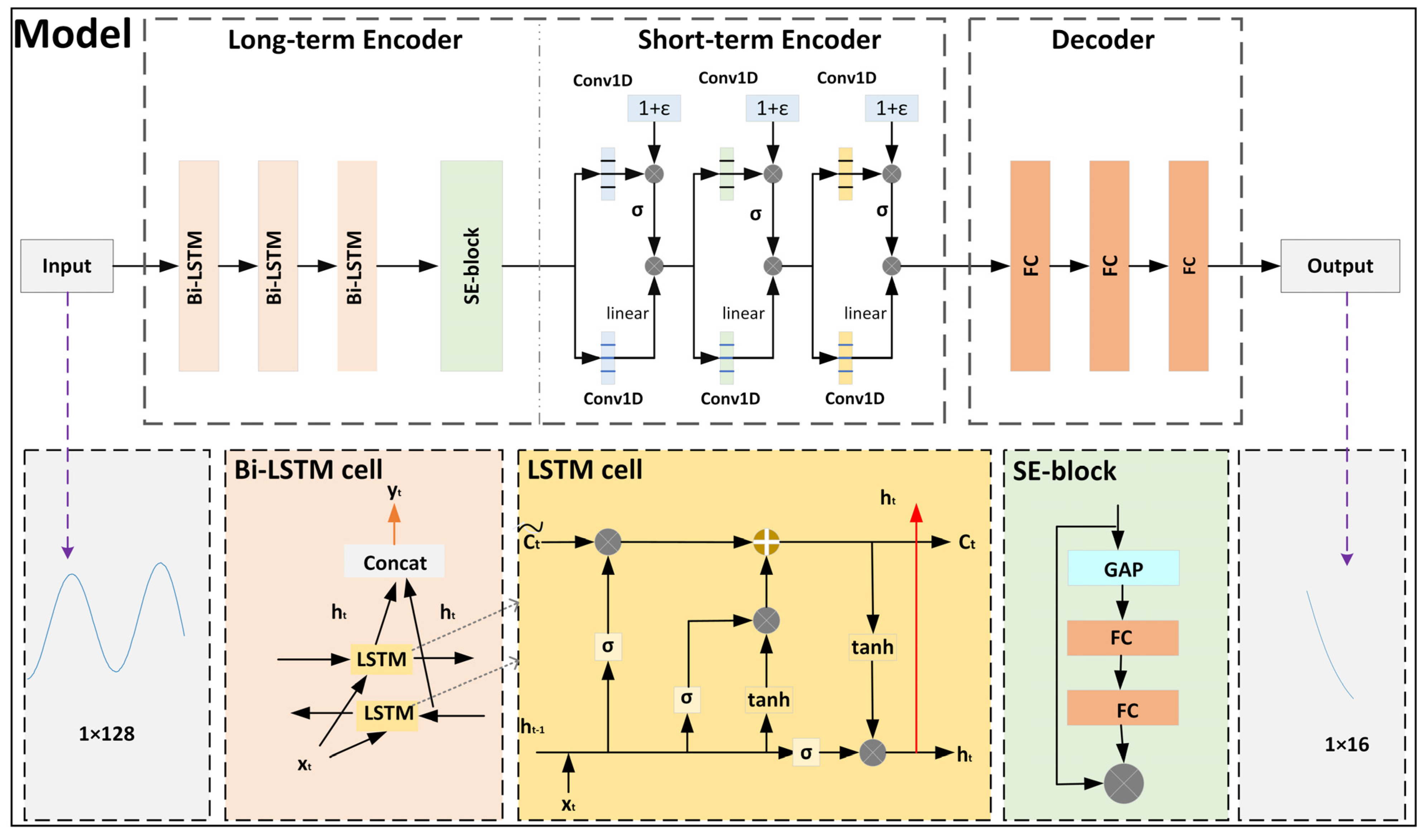
The overall architecture of the Seq2Seq network proposed in this paper is illustrated in Figure 1. It combines a stacked Bi-LSTM module with an attention-based Squeeze-Excitation (SE) block as the long-term encoder to extract long-term characteristics of heave data. Simultaneously, it utilizes a gated CNN as the short-term encoder to extract local temporal features. In addition, the decoder part of the model employs stacked fully connected (FC) layers to generate the predicted heave signal. The detailed structures of each part of the network are discussed separately below.
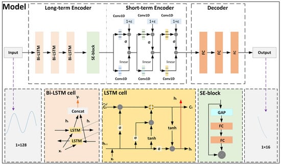
Figure 1.
Overall architecture of the proposed network.
2.1. Long-Term Encoder
In this study, we employ Bi-LSTM combined with an attention-based SE block [23] to construct a long-term encoder module. Bi-LSTM is an advanced network structure based on LSTM, originally proposed by Schuster et al. [24]. Unlike traditional unidirectional LSTM, Bi-LSTM considers both forward and backward information of the input sequence simultaneously, thus capturing the contextual relationships within the sequence more comprehensively. As shown in Figure 1, this dual perspective allows Bi-LSTM to utilize not only the past input information (left to right) but also the future input information (right to left), thereby enhancing the modeling capability for time series data.
The basic structure of an LSTM network consists of a memory block that includes a Forget Gate (FG), an Input Gate (IG), and an Output Gate (OG). These gating mechanisms enable LSTM to control the flow of information and selective forgetting. The gating units work together to determine which information needs to be retained, forgotten, updated, and output. The FG, in particular, controls which information from the previous memory cell state should be kept or discarded. It uses a sigmoid function to decide the degree of forgetting.
where is the output of the FG, represents the previous hidden state, and the current input is . The weights and bias for the FG are represented by and , respectively, and denotes the sigmoid activation function, that is
The IG updates the memory cell state by integrating the current input with the previous hidden state . It employs sigmoid and tanh functions to manage the information update, as described by the following equations:
The output of the IG is indicated by , while the weight matrix and bias are denoted by and , respectively. The candidate cell state is computed using the tanh function, , which preserves the relative relationships among input data by making larger values more distinct from smaller ones.
The cell state update is accomplished by the combined action of the FG and the IG, merging past and new information.
where represents the memory content at the current time step, storing information from both past and current inputs, and denotes element-wise multiplication.
Finally, the OG controls which information from the memory cell state is used for the current hidden state .
The output of the OG is denoted by , with and representing the weight matrix and bias, respectively.
In a Bi-LSTM, the input sequence is fed into two LSTM networks in parallel. At time step t, one network captures the forward sequence information to produce , while the other processes it in the backward direction, yielding . The outputs from these two networks are then concatenated to generate the final output. This dual-path approach allows the network to utilize information from both past and future contexts, enhancing its ability to model complex sequence dependencies.
We then employ the SE-block to improve Bi-LSTM’s capacity to model heave data by refining feature channels and better capturing temporal dependencies. It can effectively improve feature selection by weighing each feature channel to highlight key features without significantly increasing complexity. As shown in Figure 1, the SE-block comprises two main modules: the Squeeze module and the Excitation module. In the Squeeze module, the network captures the global information of each channel through Global Average Pooling (GAP). It converts the features of each channel into a single value. After processing through the Squeeze module, the model outputs a vector containing 128 elements, each representing the global features of its corresponding channel.
where is the output of the stacked Bi-LSTM.
In the Excitation module, channel relationships are comprehended via two sequential FC layers [25]. The first FC layer undertakes dimensionality reduction to simplify the model’s complexity and enhance its generalization ability. Subsequently, the second FC layer performs dimensionality expansion, reinstating the feature vector to match the dimension of the shared encoder output. Consequently, the long-term encoder’s focus on pivotal features is heightened, significantly augmenting the predictive efficacy of the proposed model.
In this study, various reduction ratios (8, 16, 32, and 64) were assessed to ensure the dimensionality reduction in the first FC layer, with the optimal ratio identified as 16. Accordingly, the first FC layer comprises 8 neurons and employs the Rectified Linear Unit (ReLU) activation function,, whereas the second FC layer includes 128 neurons and utilizes the sigmoid activation function.
where represents the ReLU activation function, and are the weights and biases of the first FC layer, and and are the weights and biases of the second FC layer.
Ultimately, by multiplying the weight vector obtained from the Excitation operation with the input feature map, the output of long-term encoder is obtained as .
The SE-enhanced long-term encoder not only boosts the model’s efficiency and stability but also maintains a low computational overhead due to its lightweight design.
2.2. Short-Term Encoder
After performing long-term feature mapping, the is fed into a short-term encoder composed of three stacked convolutional blocks, as illustrated in Figure 1. It is designed to extract multi-scale short-term features from heave data. Each convolutional block is equipped with Gated Linear Units (GLUs) [23], referred to as Gated Convolutional Layers (GCLs) in this study. The GCL function applies a gating mechanism to the outputs of traditional nonlinear activated convolutions [25]. Furthermore, to bolster the robustness of the gating mechanism, we introduce a uniform random tensor ϵ [−0.1, 0.1]. This random perturbation mechanism, inspired by [26], serves as an additional interference to the gates. It ensures that the model performs more stably in the presence of noise and uncertainty. The GCL for layer y is defined as follows:
where denotes the point-wise multiplication of the linear and nonlinear outputs of each layer, and σ represents the sigmoid activation function. The linear output represents features transformed through a linear transformation. Simultaneously, the nonlinear output is processed by the sigmoid activation function, with values ranging from 0 to 1. Subsequently, the linear output is elementwise multiplied by the gate signal vector , generating the final output vector. By adding noise to the gate signal, the proposed model becomes more robust to input data variations and less sensitive to minor fluctuations. It is important to note that the noise factor is only applied during the training phase and not during the testing phase.
All convolutional filters are designed with a kernel size of 13 × 1, allowing for shallow feature embedding extraction from . In the convolutional encoder structure, as shown in Figure 1, the number of kernels is gradually increased as 16, 32, and 64, respectively, thereby expanding the channel capacity and better representing complex data.
To reduce the spatial dimensions of the output feature maps, a stride of 2 is set in the short-term encoder. This not only helps reduce computational load but also enhances the effectiveness of feature extraction.
2.3. Decoder
The encoded feature is a 128-channel feature vector. As shown in Figure 1, we use three FC layers for data reconstruction in the decoder. The output of each FC layer can be expressed by the following formula:
where represents the output vector of the i-th layer, is the weight matrix of the i-th layer, is the input vector of the (i − 1)-th layer, and is the bias vector of the i-th layer.
In detail, the first FC layer has 128 neurons and uses the ReLU activation function. The second FC layer has 64 neurons, also using the ReLU activation function. The last FC layer has 1 neuron with a linear activation function to generate 1 dimensional 16-point length prediction values.
3. Optimization Strategy
The standard Huber loss function behaves as mean squared error when dealing with small residuals and as linear loss when handling large residuals, offering robust performance. In this study, the slope factor-optimized Huber loss function (S-HuberLoss) is introduced to enhance the ability to handle outliers and further improve model performance. The calculation of S-HuberLoss is as follows:
where denotes the original heave signal, signifies the restored signal, and represents the slope weighting factor. The symbol serves as a threshold value, marking the transition from quadratic to linear loss. Through extensive experimental comparisons, this threshold is determined to be 0.05. The introduction of S-HuberLoss adjusts the loss function by assigning different weights to various sample points, thereby enhancing the model’s flexibility in handling extremums and troughs. This improvement significantly boosts the model’s ability to fit complex ship heave motions. Especially when dealing with minor variations, S-HuberLoss effectively reduces the impact of anomalous data, such as sudden extreme sea conditions, on the model’s predictions, thereby improving its performance across a range of scenarios.
The slope weighting factor is calculated as follows:
where n is the length of the heave signal.
To achieve optimal predictive performance, this study proposes a composite loss function, combining the S-HuberLoss with the Maximum Absolute Deviation Loss (MADLoss) function for model training. The adoption of the MADLoss function enhances the model’s sensitivity to prediction errors. This adjustment aims to optimize scenarios with significant deviations, thereby improving the model’s predictive capability. The MADLoss function is characterized by its emphasis on large errors, increasing the penalty on these points to ensure the model focuses more on samples with substantial errors during training, thus enhancing its ability to handle extreme situations. With n as the length of the predicted heave signal, the computation of MADLoss is as follows:
Subsequently, the total loss of this study is as follows:
4. Experiments Settings
4.1. Datasets
This study focuses on heave data, referencing marine environmental information at specific times [27]. The specific parameters of the marine environment are shown in Table 2.
Table 2.
Wave level specifications.
The training and validation datasets used in this study were collected using the Marine Systems Simulator (MSS). MSS was selected as the primary simulator due to its open-source nature, extensibility, high-fidelity simulation, and efficient computation. We chose a S175 ship (a built-in model in MSS) with waves modeled using the JONSWAP wave spectrum based on the North Sea (Norsok) data. The peak frequency of these data was calculated as . The wave period was set to 10 s, and the wave direction angle was 30 degrees. The water depth was set to 200 m. Additionally, significant wave heights (Hs) were set at 2.5 m, 3.5 m, and 5 m, corresponding to sea states 4, 5, and 6 in Table 2. Each sea state scenario provided data for up to 100 h, with a sampling rate of 200 Hz, ensuring high-resolution temporal data.
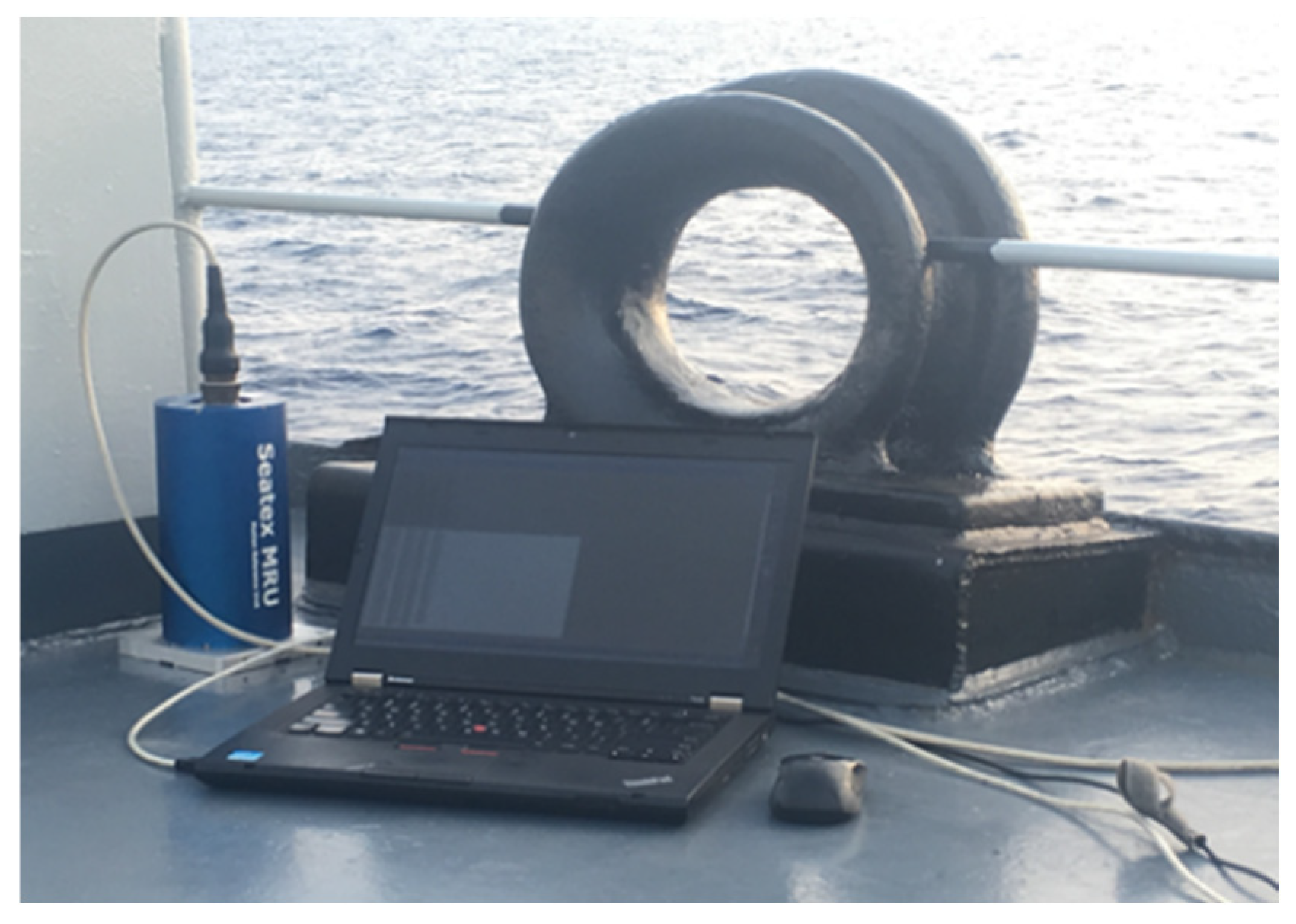
The generalized test data were collected from an actual catamaran in the South China Sea in May 2016. The Motion Reference Unit (MRU) used for data collection was Kongsberg MRU 5, and the sampling rate was set at 200 Hz, with a total sampling duration of 2000 s. The installation of the MRU and the data acquisition device is depicted in Figure 2. The measurement conditions were conducted in open waters under moderate weather. The equipment was securely installed in a fixed position on the vessel, with a wave direction angle of 30° and a measurement period of 10 s, carefully aligned with the ship’s coordinate system, and calibrated before data collection. The ship characteristics and MRU-related parameters are shown in Table 3 and Table 4, respectively.
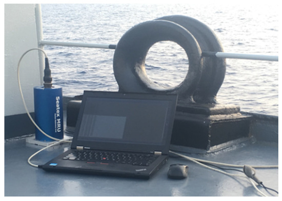
Figure 2.
The MRU and data recording device equipped on the experimental ship.
Table 3.
Experimental hull-related parameters.
Table 4.
MRU-related parameters.
To enhance the robustness and realism of the model, additive white Gaussian noise (AWGN) was introduced into the simulated data. This step was crucial for simulating real-world noise conditions and assessing the model’s performance in noisy environments. For the collected real ship data, we employed cubic spline interpolation and moving average filter to mitigate the impact of missing data points and remove noise and outliers, respectively.
4.2. Modeling Experimental Design
To assess the performance of the proposed model, we substituted the baseline model with LSTM, GRU, and bidirectional GRU (Bi-GRU) for an effective evaluation while maintaining the overall framework and experimental parameters unchanged. All algorithms were trained and tested using the same training set, validation set, test set, and standard desktop CPU resources. The data from the three sea states were divided into training and validation sets in a 7:3 ratio after segmentation and shuffling, while the evaluation test data comprised a one-hour separate dataset not included in the model training. TensorFlow 2.16.1 was employed as the training platform for the experiments.
4.3. Performance Evaluation Metrics
To evaluate the performance of the proposed model, this paper employs the following three criteria: Root Mean Squared Error (RMSE), Mean Absolute Error (MAE), and Mean Absolute Percentage Error (MAPE). These metrics are defined as follows:
where denotes the actual signal values, stand for the corresponding predicted value, and N denotes the number of data points.
RMSE reflects how well the model manages larger errors, while MAE provides an overall measure of prediction accuracy, and MAPE assesses the error relative to the actual values. Smaller values for RMSE, MAE, and MAPE indicate that the model is highly accurate and reliable.
4.4. Hyperparameter Setting
The proposed model in this study consists of five main components: input, long-term encoder, short-term encoder, decoder, and output. To achieve the optimal balance between the model’s performance and complexity, each component’s hyperparameters have been carefully optimized. The optimization method for each hyperparameter involves adjusting the relevant parameters while keeping others constant to achieve the best predictive performance. To reduce the model’s complexity, all data were down-sampled to 10 Hz during the training process. The optimal hyperparameters for each component and the training process are shown in Table 5 and Figure 1.
Table 5.
Hyperparameter setting in the proposed model.
5. Results and Discussion
This section provides a comprehensive evaluation of the proposed model from multiple perspectives. Initially, the significance and superiority of the proposed model are demonstrated through a comparative performance analysis with three baseline methods. Subsequently, the model’s efficacy is evaluated across various time steps to assess its capability to handle data with different temporal spans. Finally, extensive generalization tests are conducted using real-world datasets for multi-step forecasting to validate the model’s generalization ability on unseen data, thereby ensuring its reliability and practical applicability.
5.1. Prediction Performance of Different Methods
We evaluated our model using one hour of simulated data and compared its performance to the Bi-GRU, GRU, and LSTM models. The prediction interval was set to 0.1 s. Performance metrics were obtained by calculating the discrepancies between predicted values and actual values across the entire test dataset. The results of all metrics are presented in Table 6. It is significant to note that our proposed model surpassed the other three models in all performance metrics, with RMSE, MAE, and MAPE as 0.0045 m, 0.0035 m, and 4.6809%, respectively. Comparatively, LSTM-based model achieved the second-best RMSE, MAE, and MAPE values.
Table 6.
Model comparison.
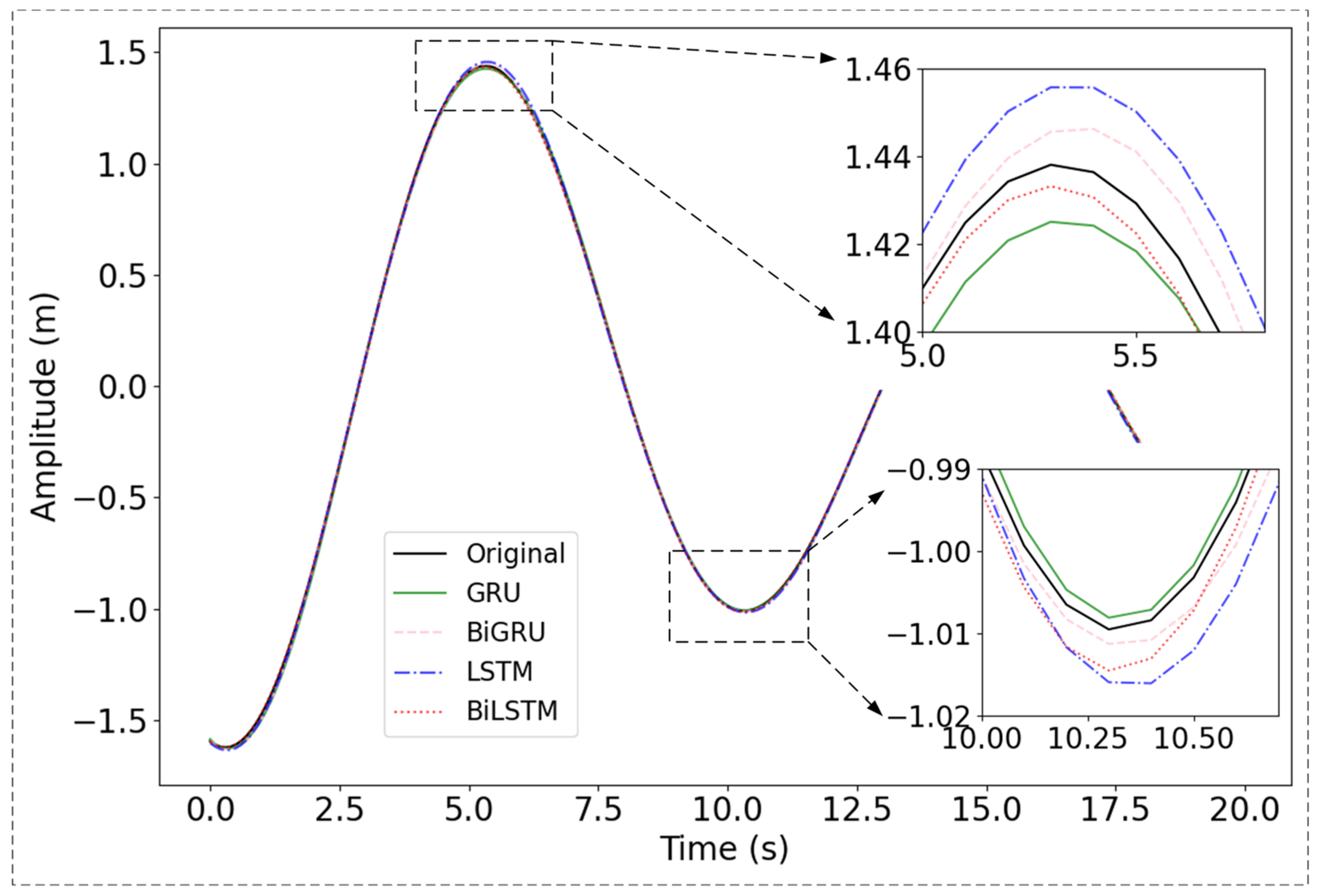
To visually assess the predictive performance of the proposed Bi-LSTM-based model comparing the baseline method, the initial 20 s segment of heave motion data was selected for analysis, as depicted in Figure 3. All methods exhibit slightly lower prediction accuracy at the peaks and troughs compared to other parts of the data. However, the maximum error range remains below 0.02 m, satisfying the technical criteria for heave compensation. This improvement is attributed to the combined use of the S-HuberLoss function and the MADLoss function. In contrast, our proposed Bi-LSTM method demonstrates the best relative performance in fitting the peak values. Overall, the proposed model, extracting both short-term and long-term features from the heave signal, allows it to closely fit the non-peak and non-trough portions to the original data while accurately capturing the peak and trough regions.
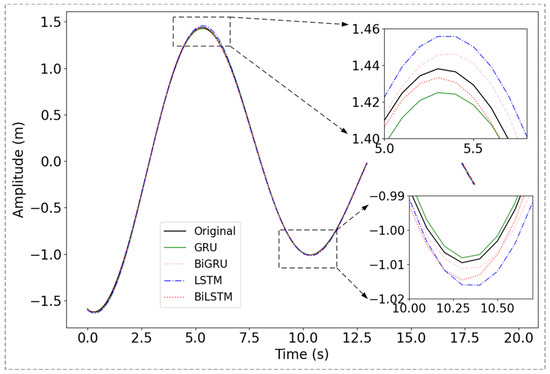
Figure 3.
Comparison of different prediction methods. The black line represents the original signal. The green, pink, blue and red lines represent the predictions made by the proposed GRU, Bi-GRU, LSTM, and Bi-LSTM, respectively.
5.2. Prediction at Different Time Steps
This study evaluated the model’s predictive performance using intervals of 0.1 s, 0.2 s, 0.5 s, and 1 s to cater to different application scenarios. As shown in Table 7, the lowest RMSE of 0.0045 m was achieved with the 0.1 s interval, indicating minimal deviation from the actual values. As the interval lengthens, the MAPE increases from 4.6809% to 4.8291%, 5.3928%, and 7.6876% for 0.2 s, 0.5 s, and 1.0 s, respectively, highlighting a decline in prediction accuracy with longer intervals. The trends of RMSE and MAE generally follow the same pattern as the time step varies. However, at the 1.0 s time step, the RMSE and MAE of the proposed method are comparable to those at the 0.2 s time step. This observation is likely influenced by the periodic nature of the heave data.
Table 7.
Prediction comparison of different time steps using the proposed model.
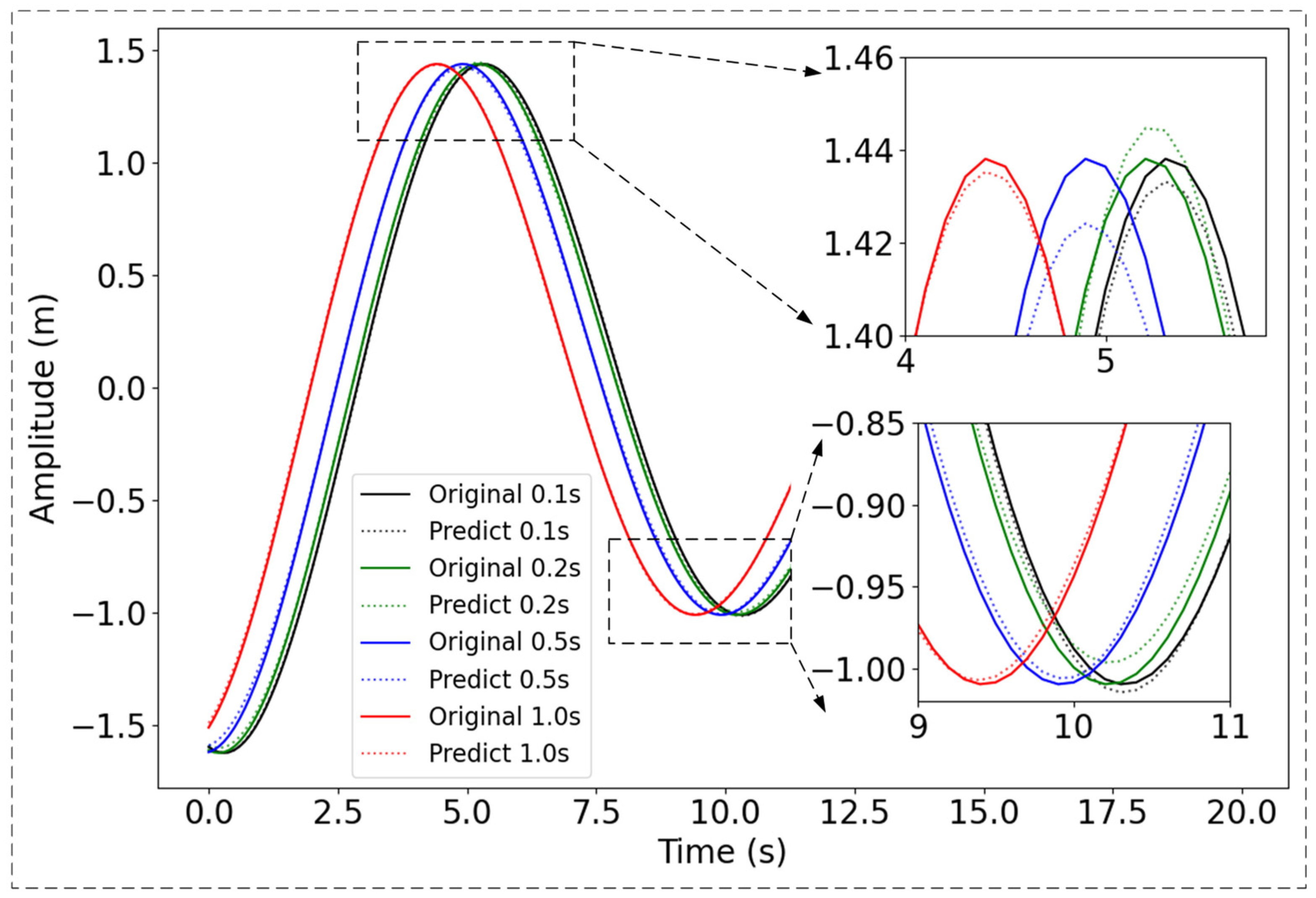
In addition, we visualized the prediction results for various time steps of the test data ranging from 0 s to 20 s, as illustrated in Figure 4. It is evident that all prediction intervals accurately follow the fundamental pattern of the original signal, demonstrating the model’s effectiveness for real-time prediction applications. Notably, even for 1.0 s time step predictions, the absolute errors for all instances remain below 0.02 m.
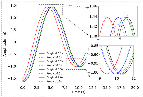
Figure 4.
Prediction at different time steps. The black, green, blue and red solid line depicts the original signal at steps 0.1 s, 0.2 s, 0.5 s, and 1 s. The dashed lines represent the corresponding prediction.
5.3. Optimization Factor Setting for S-HuberLoss
As shown in Equation (11), δ is the threshold used to switch from quadratic loss to linear loss in the S-HuberLoss function. We tested δ values of 0.01, 0.02, and 0.10 to determine the optimal setting. All performance metrics were calculated by measuring the deviation between the predicted values and the actual values for the entire test dataset. Table 8 shows that δ = 0.05 yields the lowest RMSE of 0.0045 m and MAE of 0.0035, indicating the best model performance. In comparison, δ = 0.01 produces the highest RMSE of 0.0069 m, signifying larger prediction errors, although it achieves a lower MAPE. Based on this comprehensive evaluation, δ = 0.05 was ultimately selected as the optimal value for δ to achieve the best model performance.
Table 8.
Evaluation of prediction accuracy for different δ values in S-HuberLoss.
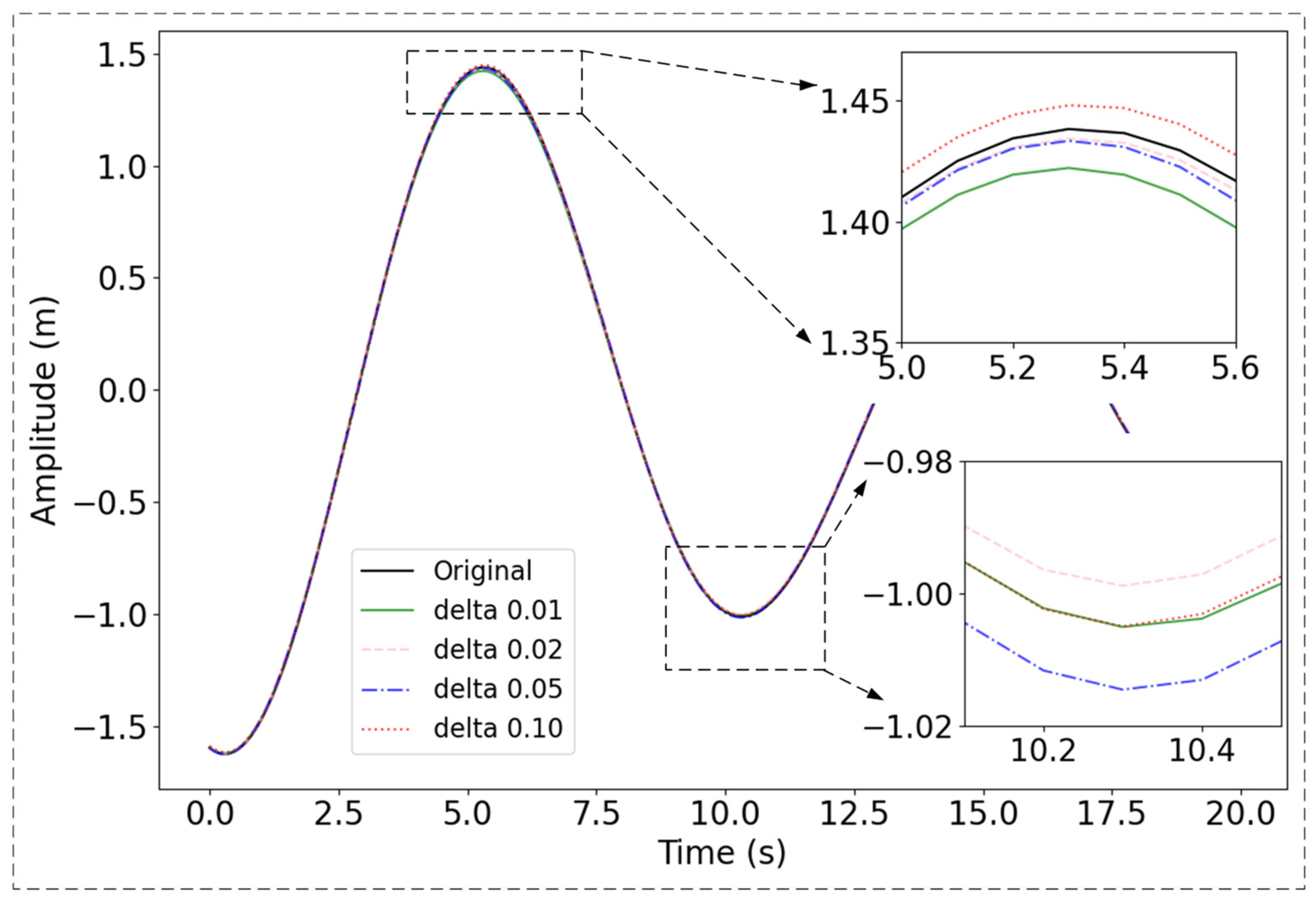
To intuitively compare the prediction performance of different δ parameters, we also plotted the prediction results for the test data from 0 s to 20 s under various δ settings. As shown in Figure 5, the overall prediction performance was optimal when δ was set to 0.05, whereas it is least effective when δ was set to 0.01. Notably, the δ value of 0.05 achieves superior performance in predicting peaks, though it is slightly less effective at predicting valleys.
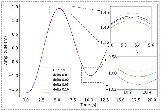
Figure 5.
Comparison of different prediction δ (delta in the figure). The black line represents the original signal. The green, pink, blue and red lines represent the predictions made by the proposed 0.01, 0.02, 0.05, and 0.10, respectively.
5.4. Generalization Testing on Real Collected Heave Data
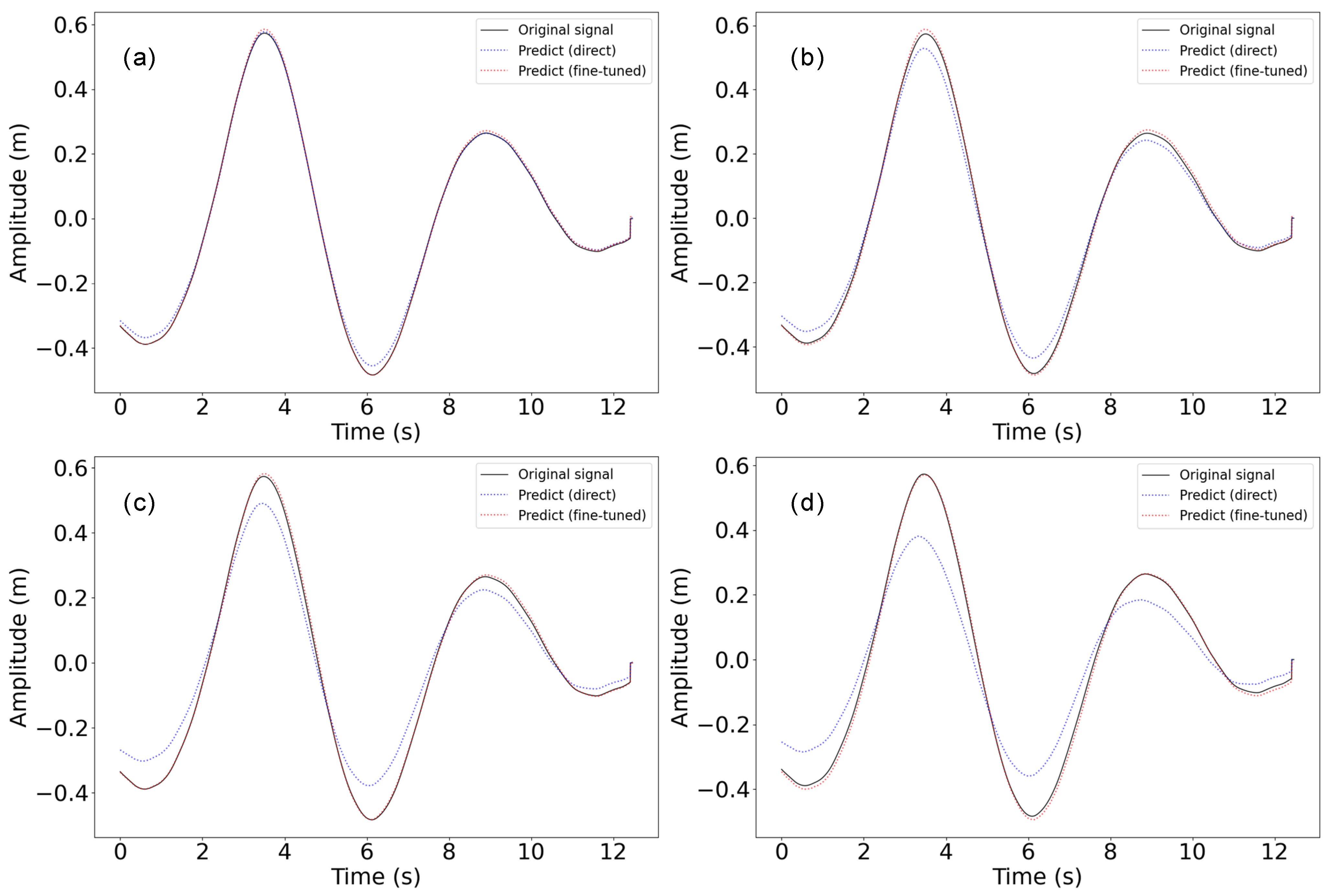
After pretraining the proposed model using simulated data under various sea conditions, we conducted generalization tests using real ship data, as detailed in Section 4.1. Initially, we directly applied the pretrained model for generalization testing without any fine-tuning. Simulation data are generated under controlled and repeatable conditions, which may include model errors and numerical inaccuracies. The characteristics of the data tend to be smoother and more regular, lacking sudden changes and random details. Due to differences in ship parameters and wave conditions, the direct generalization effect was not ideal, as shown in Figure 6 and Table 9. To address these discrepancies, we employed transfer learning, a technique that leverages a pre-trained model for a new task to enhance performance. Fine-tuning in transfer learning involves several steps: loading the pre-trained model, adjusting the output layer to fit the new task, freezing certain layers to retain learned features, and training on a new dataset to adapt to the specific requirements of the new task. In our approach, we applied transfer learning by freezing all layers except the last two. This strategy preserves the foundational features and patterns learned from the initial training data while allowing the model to adapt to the new dataset’s specific characteristics. We then performed a multi-step generalization test using this fine-tuned model.
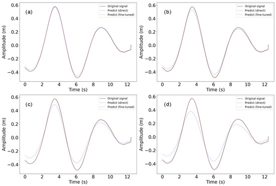
Figure 6.
Prediction visualization of different time steps with generalization test data with and without fine-tuning. (a) Prediction of 0.1 s, (b) prediction of 0.2 s, (c) prediction of 0.5 s, (d) prediction of 1 s.
Table 9.
Multi-step prediction of generalization testing data in real sea states.
As shown in Table 9, with step sizes of 0.1 s, 0.2 s, 0.5 s, and 1 s, the prediction errors after fine-tuning are mostly within 0.02 m, indicating that the generalization performance of the proposed Bi-LSTM model can meet the accuracy requirements for heave compensator in actual use. It is worth noting that with a step size of 0.1 s, the MAPE value for the direct test was slightly better than the corresponding result after fine-tuning, which has an opposite trend compared to the MAE values. These differing trends between MAE and MAPE are mainly related to the magnitude of the heave data volatility and the impact of outliers. For step sizes of 0.2 s, 0.5 s, and 1.0 s, the performance deterioration after fine-tuning becomes more noticeable. Due to hardware differences and environmental changes between different datasets, direct synthesis results may not always be satisfactory. However, after calibration with a small number of new datasets, the model can be effectively applied to data collected from real ships. In practical applications, collecting a small amount of data for fine-tuning and calibration is acceptable to achieve better prediction performance when applying the model to new ship data.
6. Conclusions
In this study, a multi-step real-time prediction model combining attention-enhanced Bi-LSTM and gated CNN is proposed, enabling efficient extraction and utilization of the temporal and global features of ship heave signal. To address the fitting distortion issue in the peak and valley part of heave data, an optimized Huber loss function with a slope factor is also proposed. Notably, in comparison to baseline methods, the proposed Bi-LSTM-based model demonstrates superior performance in predicting peaks, troughs, and other extreme points with minimal distortion. All metrics exhibit robustness across both simulated and real ship generalized test data. In addition, the inference time of the proposed model for predicting a 200 s signal is only 5.42 s using just a CPU.
While experimental results have confirmed the model’s effectiveness and usability, several significant limitations remain. For example, the proposed model was trained on simulated data and validated with a limited set of real ship data, indicating a need for more extensive real-world validation. Additionally, due to the absence of publicly available code and differing research objectives, we did not compare our model with state-of-the-art methods from previous studies. Currently, the model is still in an exploratory phase and has not yet undergone the rigorous testing required for deployment on application platforms. Further refinement is necessary to evaluate its feasibility for real-time applications.
Author Contributions
Conceptualization, W.S., Z.G., S.L. and M.C.; methodology, W.S., Z.G. and Z.D.; software, Z.G., W.S. and M.C.; validation, W.S., Z.G., Z.D. and M.C.; formal analysis, Z.G. and M.C.; investigation, W.S. and S.L.; resources, W.S. and S.L.; data curation, W.S. and Z.G.; writing—original draft preparation, W.S. and Z.G.; writing—review and editing, W.S., Z.G., Z.D., S.L. and M.C.; visualization, W.S. and Z.G.; supervision, W.S., S.L. and M.C.; project administration, W.S. and S.L.; funding acquisition, W.S. and S.L. All authors have read and agreed to the published version of the manuscript.
Funding
This research was funded by the National Natural Science Foundation of China under Grant 52175054, the Shandong Province Science and Technology-oriented Small and Medium-sized Enterprises (SMEs) Innovation Capacity Enhancement Project under Grant 2023TSGC0320 and 2022TSGC2172, and Qingdao Marine science and technology innovation project under Grant 24-1-3-hygg-5-hy.
Institutional Review Board Statement
Not applicable.
Informed Consent Statement
Not applicable.
Data Availability Statement
Dataset available upon request from the authors.
Conflicts of Interest
The authors declare no conflict of interest.
References
- Li, S.; Wu, Q.; Liu, Y.; Qiao, L.; Guo, Z.; Yan, F. Research on Three-Closed-Loop ADRC Position Compensation Strategy Based on Winch-Type Heave Compensation System with a Secondary Component. J. Mar. Sci. Eng. 2024, 12, 346. [Google Scholar] [CrossRef]
- Raven, H. A method to correct shallow-water model tests for tank wall effects. J. Mar. Sci. Technol. 2018, 24, 437–453. [Google Scholar] [CrossRef]
- Lee, J.-H.; Lee, J.; Kim, Y.; Ahn, Y. Prediction of wave-induced ship motions based on integrated neural network system and spatiotemporal wave-field data. Phys. Fluids 2023, 35, 097127. [Google Scholar] [CrossRef]
- Lee, J.; Lee, J.-H.; Kim, Y. Prediction of Nonlinear Ship Motions in Irregular Waves Based on Integrated Machine Learning Model. In Proceedings of the 33rd International Ocean and Polar Engineering Conference, Ottawa, ON, Canada, 19–23 June 2023. [Google Scholar]
- Jiang, Z.; Ma, Y.; Li, W. A Data-Driven Method for Ship Motion Forecast. J. Mar. Sci. Eng. 2024, 12, 291. [Google Scholar] [CrossRef]
- Skulstad, R.; Li, G.; Fossen, T.; Wang, T.; Zhang, H. A Co-operative Hybrid Model for Ship Motion Prediction. Model. Identif. Control: A Nor. Res. Bull. 2021, 42, 17–26. [Google Scholar] [CrossRef]
- Hou, X.; Zhou, X. Nonparametric Identification Model of Coupled Heave-Pitch Motion for Ships by Using the Measured Responses at Sea. J. Mar. Sci. Eng. 2023, 11, 676. [Google Scholar] [CrossRef]
- Skulstad, R.; Li, G.; Fossen, T.; Vik, B.; Zhang, H. A Hybrid Approach to Motion Prediction for Ship Docking—Integration of a Neural Network Model into the Ship Dynamic Model. IEEE Trans. Instrum. Meas. 2020, 70, 2501311. [Google Scholar] [CrossRef]
- Bates, M.R.; Bock, D.H.; Powell, F.D. Analog Computer Applications in Predictor Design. IRE Trans. Electron. Comput. 1957, EC-6, 143–153. [Google Scholar] [CrossRef]
- Lainiotis, D.G.; Plataniotis, K.N.; Menon, D.; Charalampous, C.J. Adaptive heave compensation via dynamic neural networks. In Proceedings of the OCEANS ’93, Victoria, BC, Canada, 18–21 October 1993; Volume 241, pp. I243–I248. [Google Scholar]
- Khan, A.; Bil, C.; Marion, K.E. Ship motion prediction for launch and recovery of air vehicles. In Proceedings of the OCEANS, Washington, DC, USA, 17–23 September 2005; Volume 1–3, pp. 2795–2801. [Google Scholar]
- Zhang, J.; Zhao, X.; Jin, S.; Greaves, D. Phase-resolved real-time ocean wave prediction with quantified uncertainty based on variational Bayesian machine learning. Appl. Energy 2022, 324, 119711. [Google Scholar] [CrossRef]
- Hu, L.; Zhang, M.; Yuan, Z.-M.; Zheng, H.; Lv, W. Predictive Control of a Heaving Compensation System Based on Machine Learning Prediction Algorithm. J. Mar. Sci. Eng. 2023, 11, 821. [Google Scholar] [CrossRef]
- Chen, Z.; Che, X.; Wang, L.; Zhang, L. Machine learning for ship heave motion prediction: Online adaptive cycle reservoir with regular jumps. Ocean Eng. 2024, 294, 116767. [Google Scholar] [CrossRef]
- Wei, Y.; Chen, Z.; Zhao, C.; Tu, Y.; Chen, X.; Yang, R. A BiLSTM hybrid model for ship roll multi-step forecasting based on decomposition and hyperparameter optimization. Ocean Eng. 2021, 242, 110138. [Google Scholar] [CrossRef]
- Zhang, T.; Zheng, X.-Q.; Liu, M.-X. Multiscale attention-based LSTM for ship motion prediction. Ocean Eng. 2021, 230, 109066. [Google Scholar] [CrossRef]
- Li, M.-W.; Xu, D.-Y.; Geng, J.; Hong, W.-C. A hybrid approach for forecasting ship motion using CNN-GRU-AM and GCWOA. Appl. Soft Comput. 2022, 114, 108084. [Google Scholar] [CrossRef]
- Sun, Q.; Tang, Z.; Gao, J.; Zhang, G. Short-term ship motion attitude prediction based on LSTM and GPR. Appl. Ocean Res. 2022, 118, 102927. [Google Scholar] [CrossRef]
- Geng, X.; Li, Y.; Sun, Q. A Novel Short-Term Ship Motion Prediction Algorithm Based on EMD and Adaptive PSO-LSTM with the Sliding Window Approach. J. Mar. Sci. Eng. 2023, 11, 466. [Google Scholar] [CrossRef]
- Zhou, T.; Yang, X.; Ren, H.; Li, C.; Han, J. The prediction of ship motion attitude in seaway based on BSO-VMD-GRU combination model. Ocean Eng. 2023, 288, 115977. [Google Scholar] [CrossRef]
- Wei, Y.; Chen, Z.; Zhao, C.; Chen, X. Deterministic ship roll forecasting model based on multi-objective data fusion and multi-layer error correction. Appl. Soft Comput. 2023, 132, 109915. [Google Scholar] [CrossRef]
- Han, C.; Hu, X. A Prediction Method of Ship Motion Based on LSTM Neural Network with Variable Step-Variable Sampling Frequency Characteristics. J. Mar. Sci. Eng. 2023, 11, 919. [Google Scholar] [CrossRef]
- Hu, J.; Shen, L.; Sun, G. Squeeze-and-Excitation Networks. In Proceedings of the 2018 IEEE/CVF Conference on Computer Vision and Pattern Recognition (CVPR), Salt Lake City, UT, USA, 18–22 June 2018; pp. 7132–7141. [Google Scholar]
- Schuster, M.; Paliwal, K.K. Bidirectional recurrent neural networks. IEEE Trans. Signal Process. 1997, 45, 2673–2681. [Google Scholar] [CrossRef]
- Chen, M.; Li, Y.; Zhang, X.; Gao, J.; Sun, Y.; Shi, W.; Wei, S. Multiscale Convolution and Attention based Denoising Autoencoder for Motion Artifact Removal in ECG Signals. In Proceedings of the 2024 7th International Conference on Image and Graphics Processing, Beijing, China, 19–21 January 2024; pp. 442–448. [Google Scholar]
- Chen, M.; Li, Y.; Zhang, L.; Zhang, X.; Gao, J.; Sun, Y.; Shi, W.; Wei, S. Multitask Learning-Based Quality Assessment and Denoising of Electrocardiogram Signals. IEEE Trans. Instrum. Meas. 2024, 73, 2510513. [Google Scholar] [CrossRef]
- GB/T 42176-2022; The Grade of Wave Height. Standards Press of China: Beijing, China, 2022.
Disclaimer/Publisher’s Note: The statements, opinions and data contained in all publications are solely those of the individual author(s) and contributor(s) and not of MDPI and/or the editor(s). MDPI and/or the editor(s) disclaim responsibility for any injury to people or property resulting from any ideas, methods, instructions or products referred to in the content. |
© 2024 by the authors. Licensee MDPI, Basel, Switzerland. This article is an open access article distributed under the terms and conditions of the Creative Commons Attribution (CC BY) license (https://creativecommons.org/licenses/by/4.0/).