
Wave–Induced Soil Dynamics and Shear Failure Potential around a Sandbar


 ,
,
Abstract
:1. Introduction
2. Materials and Methods
2.1. Wave Model
2.2. Seabed Model
2.3. Boundary Conditions
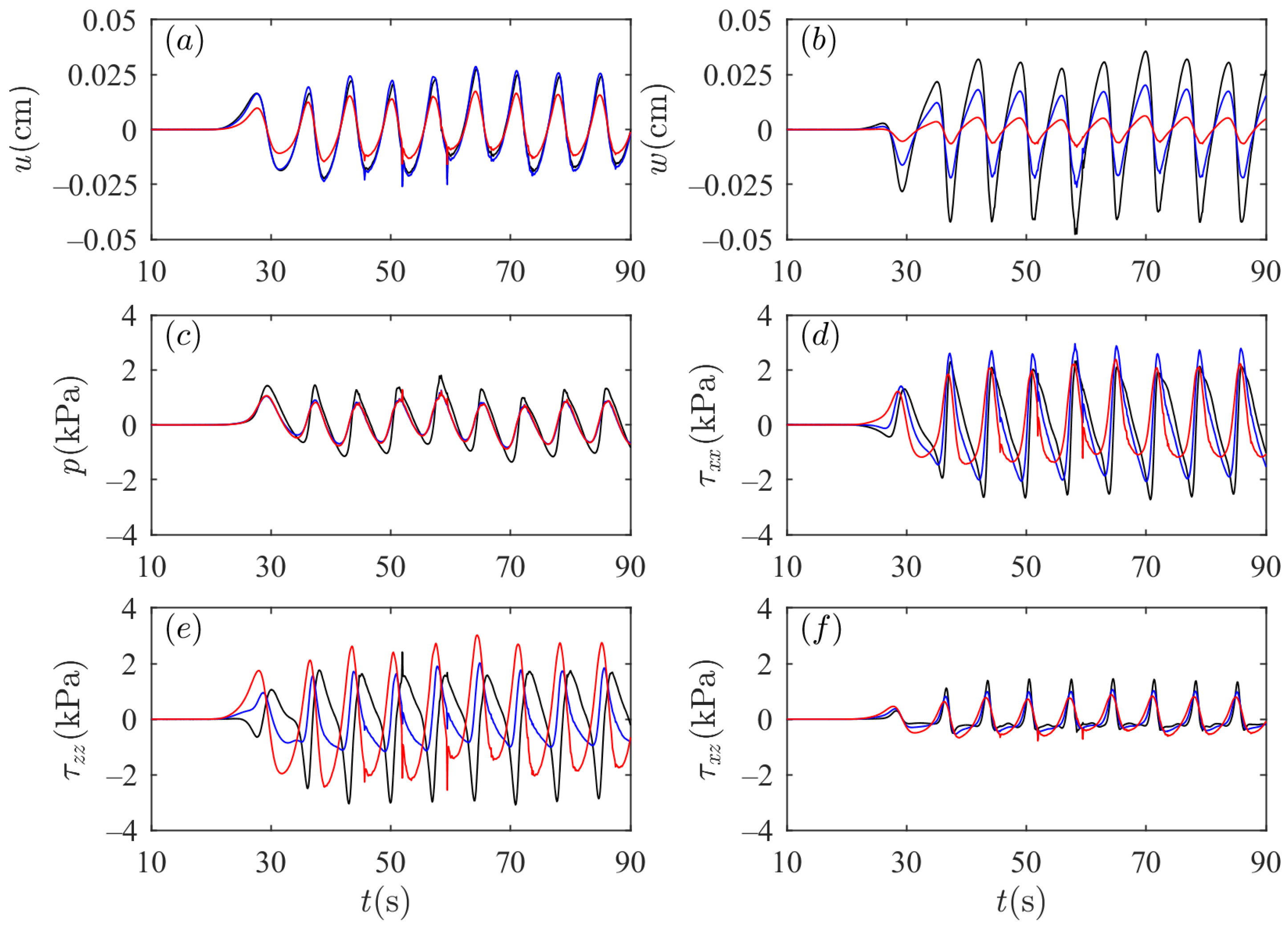
2.4. Model Coupling and Validation
3. Results and Discussion
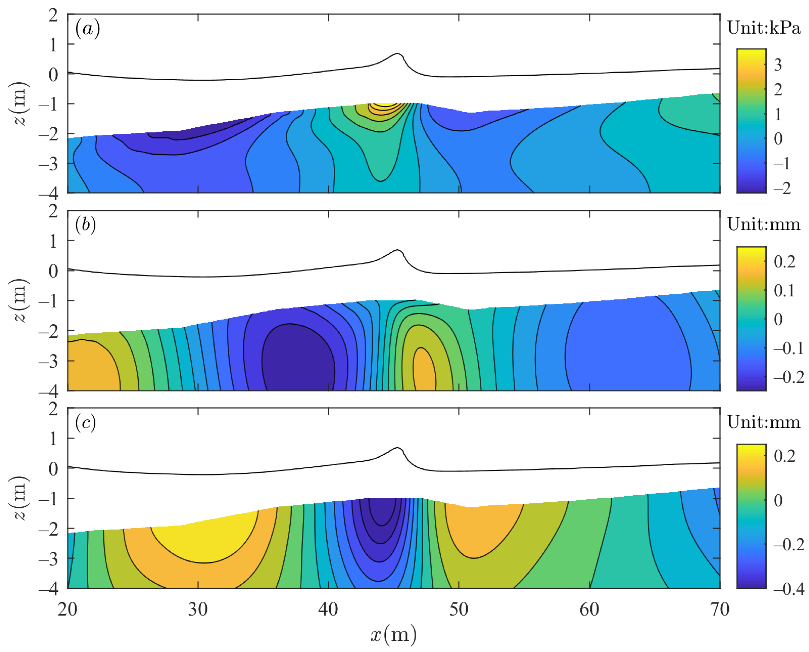
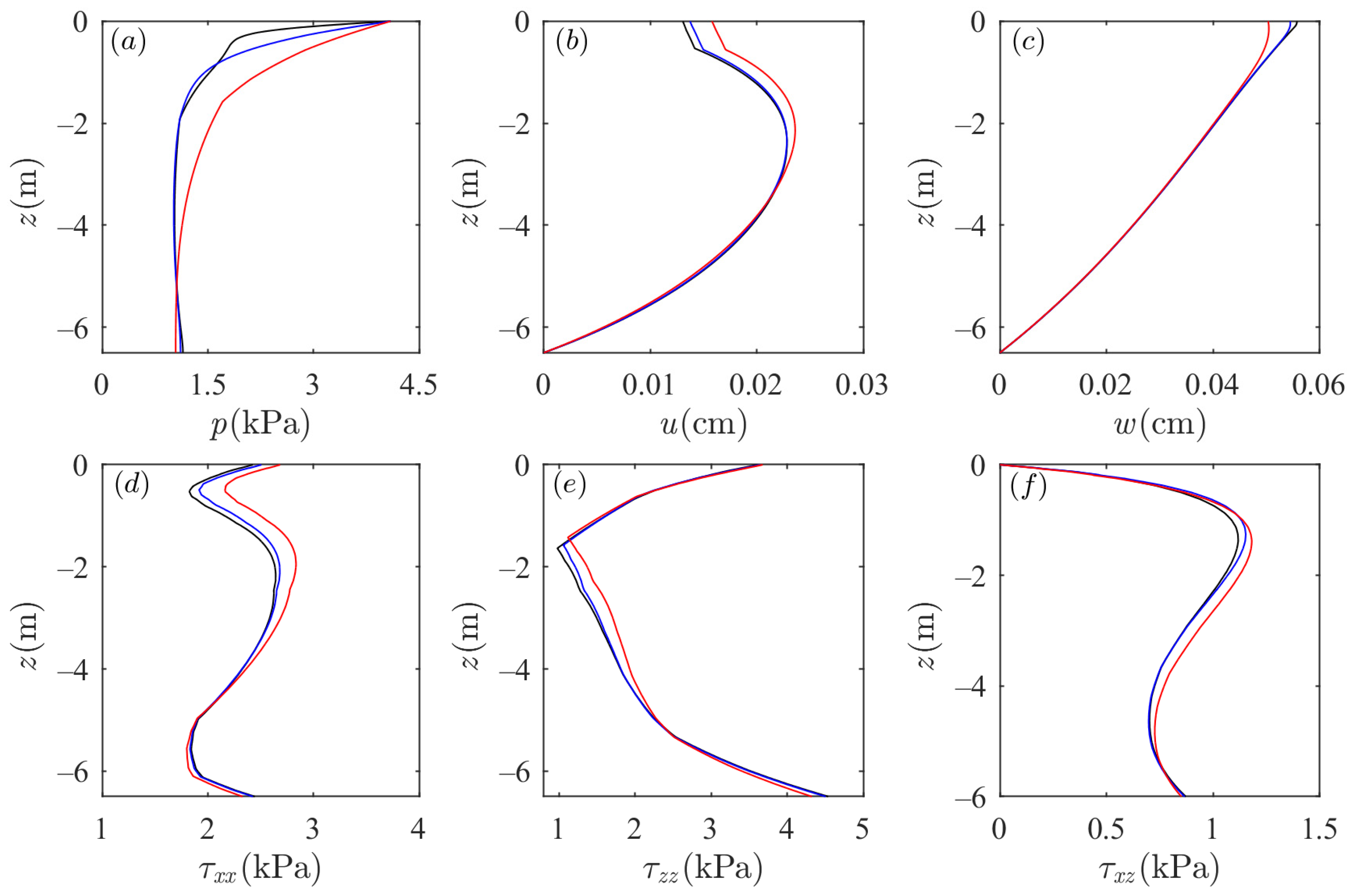
3.1. Effects of Wave Characteristics on Soil Dynamics around the Sandbar
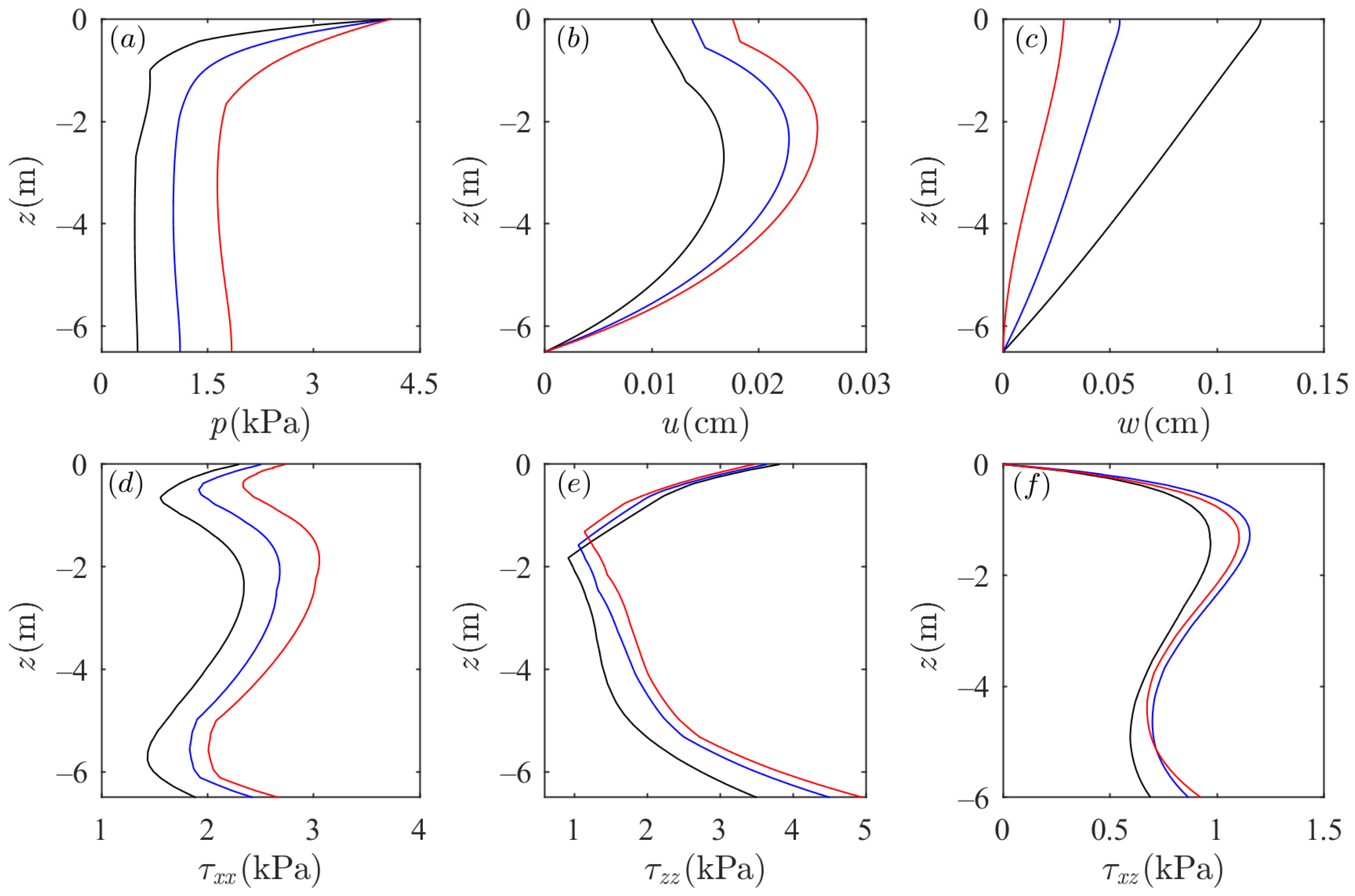
3.2. Effects of Seabed Conditions on Soil Dynamics around the Sandbar
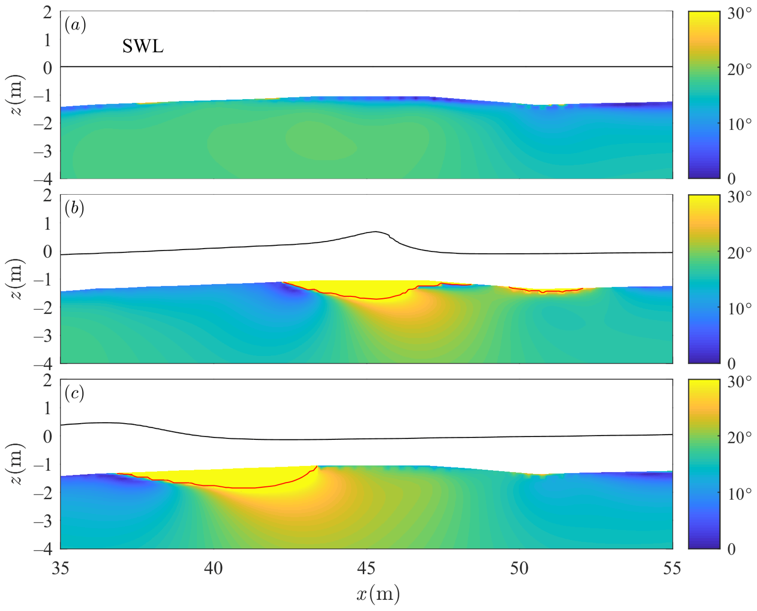
3.3. Wave-Induced Shear Failure around the Sandbar
4. Conclusions
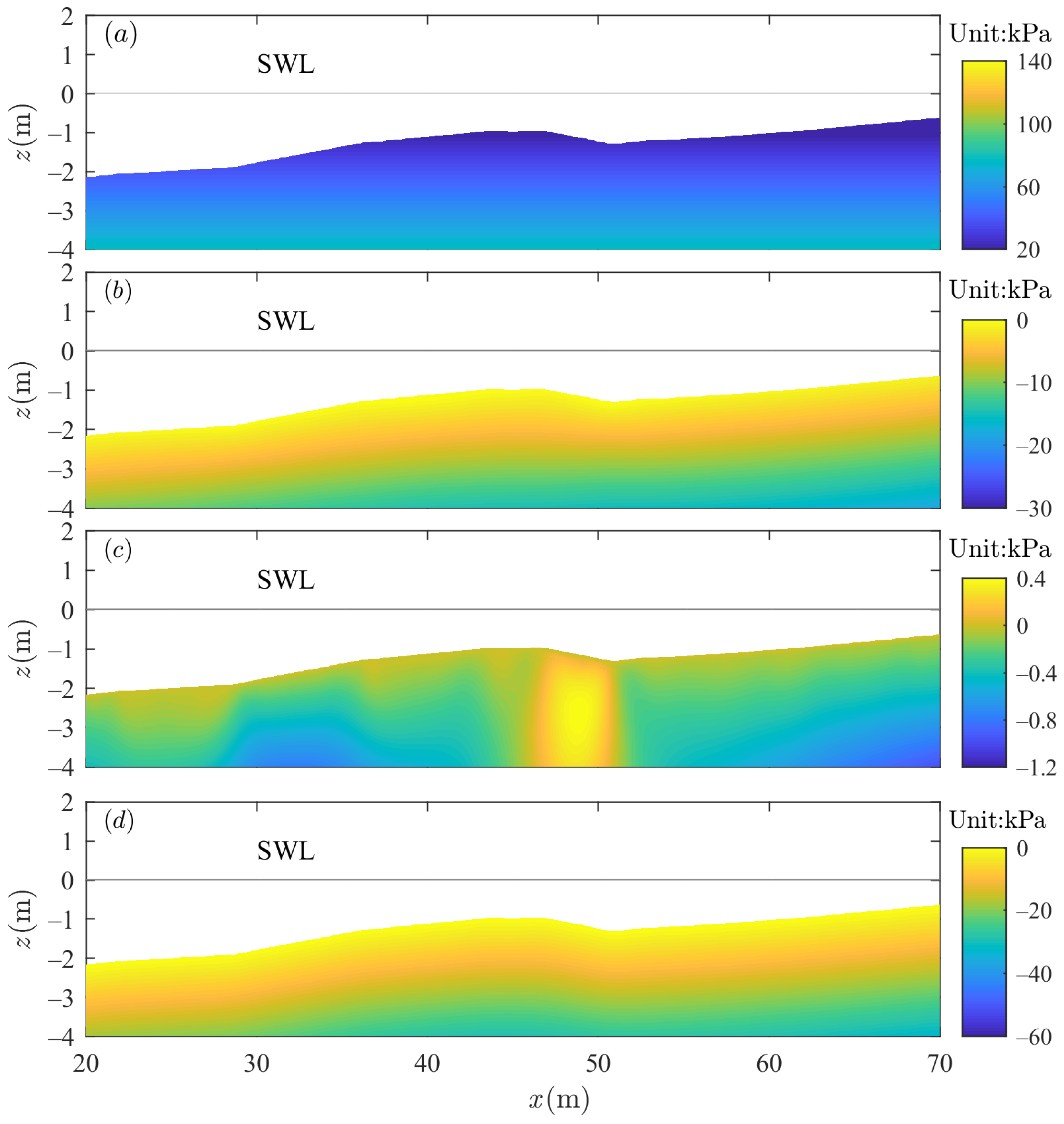
- The vertical distribution of the maximum vertical effective stress in the sandbar differs from that in the flat seabed, which is inferred to be affected by wave shoaling. The vertical effective stress inside the sandbar decreases rapidly and then grows gradually along the soil depth.
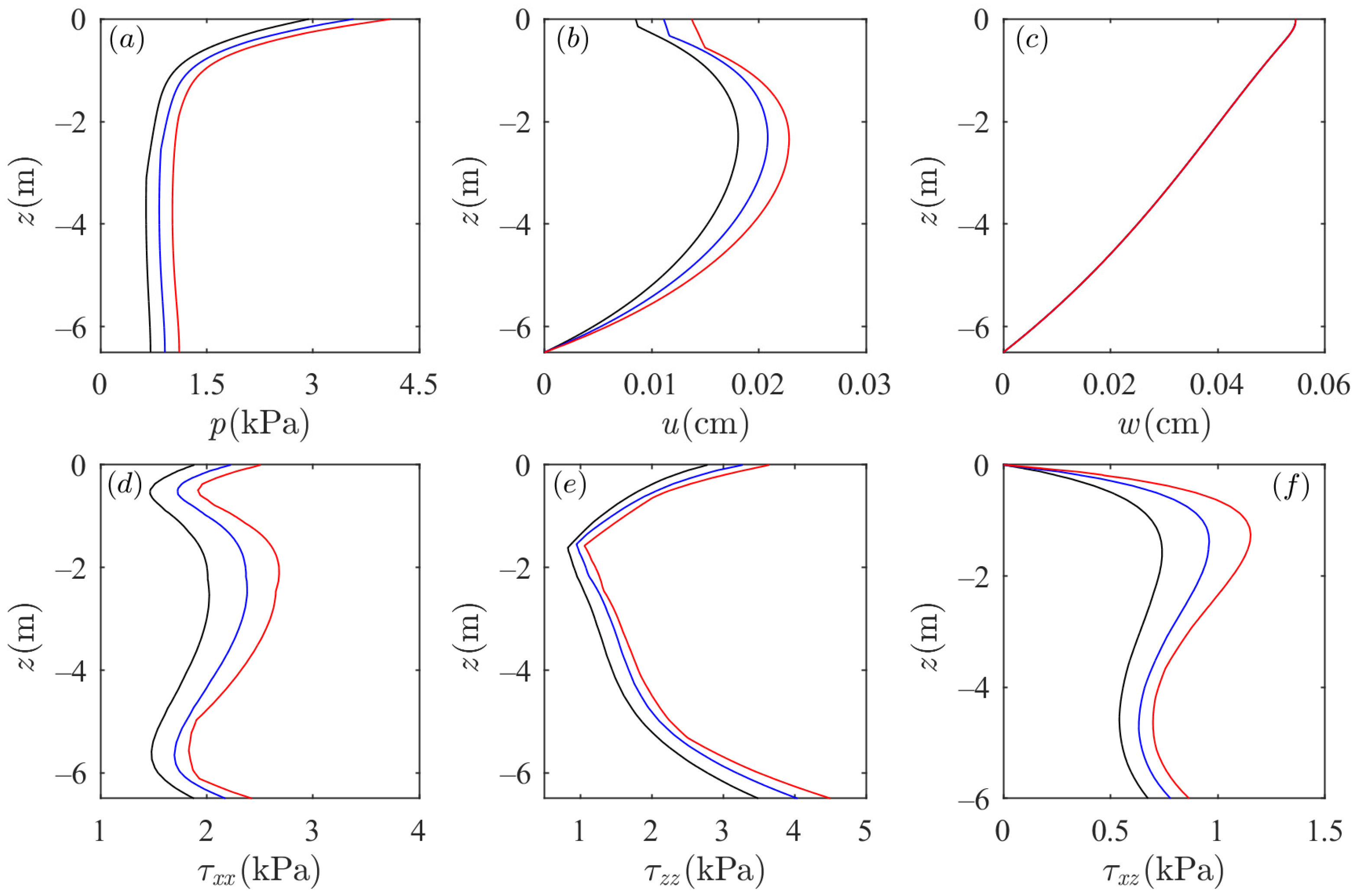
- The soil response in the sandbar is affected by wave conditions. In addition to the vertical displacement of soil particles, the soil response in the sandbar increases as wave period and wave height increase. The horizontal displacement of soil particles is not affected by the wave conditions. In addition, the soil response in the sandbar is more sensitive to the change in wave period than that of wave height. It is worth noting that the impact of wave period on the vertical distribution of shear stress in the sandbar is different from that on the flat seabed.
- Soil properties also play a crucial role in soil response around the sandbar. The soil response increases as the soil permeability coefficient grows except for the vertical displacement of soil particles. With the increase in soil permeability coefficient, the vertical displacement of shallow soil particles declines, while the vertical displacement of deeper soil particles is unaffected. With increasing soil shear modulus, the pore pressure, soil particle displacement, and horizontal effective stress decrease, while the shear stress and vertical effective stress increase first and then decrease as soil depth increases. Additionally, when initial soil saturation increases, the pore pressure, soil particle horizontal displacement, and horizontal effective stress increase, and soil particle vertical displacement slightly decreases. The vertical effective stress decreases first and then increases as soil depth increases. As the soil saturation grows, the shear stress inside the seabed soil increases and then decreases. Unlike the flat seabed, the vertical distribution of the vertical effective stress inside the sandbar increases as soil permeability increases, declines first, and then increases as soil saturation increases.
- The sandbar soil shear failure potential is discussed according to the Mohr–Coulomb criterion. The sandbar undergoes shear failure during the wave propagation. The range of shear failure around the sandbar is wider and the depth is deeper when the wave trough arrives.
Author Contributions
Funding
Institutional Review Board Statement
Informed Consent Statement
Data Availability Statement
Conflicts of Interest
References
- Reguero, B.G.; Losada, I.J.; Méndez, F.J. A Recent Increase in Global Wave Power as a Consequence of Oceanic Warming. Nat. Commun. 2019, 10, 205. [Google Scholar] [CrossRef] [PubMed]
- Shi, J.; Feng, X.B.; Toumi, R.; Zhang, C.; Hodges, K.I.; Tao, A.F.; Zhang, W.; Zheng, J.H. Global Increase in Tropical Cyclone Ocean Surface Waves. Nat. Commun. 2024, 15, 174. [Google Scholar] [CrossRef] [PubMed]
- Gallagher, E.L.; Elgar, S.; Guza, R.T. Observations of sand bar evolution on a natural beach. J. Geophys. Res. Ocean. 1998, 103, 3203–3215. [Google Scholar] [CrossRef]
- Anderson, D.L.; Bak, A.S.; Cohn, N.; Brodie, K.L.; Johnson, B.B.; Dickhudt, P. The Impact of Inherited Morphology on Sandbar Migration During Mild Wave Seasons. Geophys. Res. Lett. 2023, 50, e2022GL101219. [Google Scholar] [CrossRef]
- Yu, J.; Mei, C.C. Formation of Sand Bars under Surface Waves. J. Fluid Mech. 2000, 416, 315–348. [Google Scholar] [CrossRef]
- Liu, P.L.-F.; Chan, I.C. On Long-wave Propagation over a Fluid-mud Seabed. J. Fluid Mech. 2007, 579, 467–480. [Google Scholar] [CrossRef]
- Liu, Z.; Jeng, D.-S.; Chan, A.H.C.; Luan, M. Wave-induced Progressive Liquefaction in a Poro-elastoplastic Seabed: A Two-layered Model. Int. J. Numer. Anal. Methods Geomech. 2009, 33, 591–610. [Google Scholar] [CrossRef]
- Liu, X.L.; Chai, N.; Zhao, H.Y.; Jeng, D.-S.; Zhou, J. Numerical Investigation into Wave-induced Progressive Liquefaction Based on a Two-layer Viscous Fluid System. Comput. Geotech. 2023, 159, 105447. [Google Scholar] [CrossRef]
- Baldock, T.E.; Baird, A.J.; Horn, D.P.; Mason, T. Measurements and Modeling of Swash-induced Pressure Gradients in the Surface Layers of a Sand Beach. J. Geophys. Res. Ocean. 2001, 106, 2653–2666. [Google Scholar] [CrossRef]
- Mason, H.B.; Yeh, H. Sediment Liquefaction: A Pore-water Pressure Gradient Viewpoint. Bull. Seismol. Soc. Am. 2006, 106, 1908–1913. [Google Scholar] [CrossRef]
- Anderson, D.; Cox, D.; Mieras, R.; Puleo, J.A.; Hsu, T.-J. Observations of Wave-induced Pore Pressure Gradients and Bed Level Response on a Surf Zone Sandbar. J. Geophys. Res. Ocean. 2017, 122, 5169–5193. [Google Scholar] [CrossRef]
- Tong, L.; Zhang, J.; Zhao, J.; Zheng, J.; Guo, Y. Modelling Study of Wave Damping over a Sandy and a Silty Bed. Coast. Eng. 2020, 161, 103756. [Google Scholar] [CrossRef]
- Yamamoto, T. Wave-induced Pore Pressures and Effective Stresses in Inhomogeneous Seabed Foundations. Ocean Eng. 1981, 8, 1–16. [Google Scholar] [CrossRef]
- Jeng, D.-S.; Rahman, M.S. Effective Stresses in a Porous Seabed of Finite Thickness: Inertia Effects. Can. Geotech. J. 2000, 37, 1383–1392. [Google Scholar] [CrossRef]
- Jeng, D.-S.; Cha, D.H. Effects of Dynamic Soil Behavior and Wave Non-linearity on the Wave-induced Pore Pressure and Effective Stresses in Porous Seabed. Ocean Eng. 2003, 30, 2065–2089. [Google Scholar] [CrossRef]
- Ren, Y.; Xu, X.; Zhao, T.; Wang, X. The Initial Wave Induced Failure of Silty Seabed: Liquefaction or Shear Failure. Ocean Eng. 2020, 200, 106990. [Google Scholar] [CrossRef]
- King, C.A.; Williams, W.W. The Formation and Movement of Sand Bars by Wave Action. Geogr. J. 1949, 113, 70. [Google Scholar] [CrossRef]
- Benjamin, T.B.; Boczar-Karakiewicz, B.; Pritchard, W.G. Reflection of Water Waves in a Channel with Corrugated Bed. J. Fluid Mech. 1987, 185, 249–274. [Google Scholar] [CrossRef]
- Reniers, A.J.; Thornton, E.B.; Stanton, T.; Roelvink, J.A. Vertical Flow Structure during Sandy Duck: Observations and Modeling. Coast. Eng. 2004, 51, 237–260. [Google Scholar] [CrossRef]
- Cohn, N.; Ruggiero, P.; Oritiz, J.; Walstra, D.J. Investigating the Role of Complex Sandbar Morphology on Nearshore Hydrodynamics. J. Coast. Res. 2014, 70, 53–58. [Google Scholar] [CrossRef]
- Chiapponi, L.; Cobos, M.; Losada, M.A.; Longo, S. Cross-shore Variability and Vorticity Dynamics during Wave Breaking on a Fixed Bar. Coast. Eng. 2017, 127, 119–133. [Google Scholar] [CrossRef]
- Van der, A.D.A.; Van der Zanden, J.; O’Donoghue, T.; Hurther, D.; Cáceres, I.; McLelland, S.J.; Ribberink, J.S. Large-scale Laboratory Study of Breaking Wave Hydrodynamics over a Fixed Bar. J. Geophys. Res. Ocean. 2017, 122, 3287–3310. [Google Scholar] [CrossRef]
- Van der Zanden, J.; Van der, A.D.A.; Cáceres, I.; Hurther, D.; McLelland, S.J.; Ribberink, J.S.; O’Donoghue, T. Near-bed Turbulent Kinetic Energy Budget under a Large-scale Plunging Breaking Wave over a Fixed Bar. J. Geophys. Res. Ocean. 2018, 123, 1429–1456. [Google Scholar] [CrossRef]
- Mulligan, R.P.; Gomes, E.R.; Miselis, J.L.; McNinch, J.E. Non-hydrostatic Numerical Modelling of Nearshore Wave Transformation over Shore-oblique Sandbars. Estuar. Coast. Shelf Sci. 2019, 219, 151–160. [Google Scholar] [CrossRef]
- Larsen, B.E.; Van der, A.D.A.; Van der Zanden, J.; Ruessink, G.; Fuhrman, G.R. Stabilized RANS Simulation of Surf Zone Kinematics and Boundary Layer Processes beneath Large-scale Plunging Waves over a Breaker Bar. Ocean Model. 2020, 155, 101705. [Google Scholar] [CrossRef]
- Wang, J.; Wang, T.; Xing, F.; Wu, H.; Jia, J.; Yang, Z.; Wang, Y. Internal Waves Triggered by River Mouth Shoals in the Yangtze River Estuary. Ocean Eng. 2020, 214, 107828. [Google Scholar] [CrossRef]
- Fang, H.Q.; Tang, L.; Lin, P.Z. Bragg scattering of nonlinear surface waves by sinusoidal sandbars. J. Fluid Mech. 2024, 979, A13. [Google Scholar] [CrossRef]
- Gao, J.L.; Ma, X.Z.; Dong, G.H.; Chen, H.Z.; Liu, Q.; Zang, J. Investigation on the effects of Bragg reflection on harbor oscillations. Coast. Eng. 2021, 170, 103977. [Google Scholar] [CrossRef]
- Gao, J.L.; Shi, H.B.; Zang, J.; Liu, Y.Y. Mechanism analysis on the mitigation of harbor resonance by periodic undulating topography. Ocean Eng. 2023, 281, 114923. [Google Scholar] [CrossRef]
- Gao, J.L.; Hou, L.H.; Liu, Y.Y.; Shi, H.B. Influences of bragg reflection on harbor resonance triggered by irregular wave groups. Ocean Eng. 2024, 305, 117941. [Google Scholar] [CrossRef]
- Liu, P.L.-F.; Park, Y.S.; Lara, J.L. Long-wave-induced flows in an unsaturated permeable seabed. J. Fluid Mech. 2007, 586, 323–345. [Google Scholar] [CrossRef]
- Carraro, T.; Goll, C.; Marciniak-Czochra, A.; Mikelić, A. Pressure jump interface law for the Stokes–Darcy coupling: Confirmation by direct numerical simulations. J. Fluid Mech. 2013, 732, 510–536. [Google Scholar] [CrossRef]
- Biot, M.A. General theory of three-dimensional consolidation. J. Appl. Phys. 1941, 12, 155–164. [Google Scholar] [CrossRef]
- Jeng, D.-S. Wave-induced sea floor dynamics. Appl. Mech. Rev. 2003, 56, 407–429. [Google Scholar] [CrossRef]
- Yamamoto, T.; Koning, H.L.; Sellmejjer, H.; Hijum, H.L. On the response of a poro-elastic bed to water waves. J. Fluid Mech. 1978, 87, 193–206. [Google Scholar] [CrossRef]
- Jeng, D.-S.; Hsu, J.R.C. Wave-induced soil response in a nearly saturated sea-bed of finite thickness. Géotechnique 1996, 46, 427–440. [Google Scholar] [CrossRef]
- Jeng, D.-S.; Seymour, B.R. Response in seabed of finite depth with variable permeability. J. Geotech. Geoenviron. Eng. 1997, 123, 9–19. [Google Scholar] [CrossRef]
- Xu, L.Y.; Chen, W.Y.; Zhao, K.; Cai, F.; Zhang, J.Z.; Chen, G.X.; Jeng, D.-S. Poro-elastic and Poro-elasto-plastic Modeling of Sandy Seabed under Wave Action. Ocean Eng. 2022, 260, 112002. [Google Scholar] [CrossRef]
- Tong, L.L.; Zhang, J.S.; Chen, N.; Lin, X.F.; He, R.; Sun, L. Internal solitary wave-induced soil responses and its effects on seabed instability in the South China Sea. Ocean Eng. 2024, 310, 118697. [Google Scholar] [CrossRef]
- Zhao, H.Y.; Liang, Z.D.; Jeng, D.-S.; Zhu, J.F.; Guo, Z.; Chen, W.Y. Numerical investigation of dynamic soil response around a submerged rubble mound breakwater. Ocean Eng. 2018, 156, 406–423. [Google Scholar] [CrossRef]
- Rafati, Y.; Hsu, T.J.; Elgar, S.; Raubenheimer, B.; Quataert, E.; Van Dongeren, A. Modeling the hydrodynamics and morphodynamics of sandbar migration events. Coast. Eng. 2021, 166, 103885. [Google Scholar] [CrossRef]
- Patrick, M.; Chauchat, J.; Shafiei, H.; Almar, R.; Benshila, R.; Dumas, F.; Debreu, L. 3D wave-resolving simulation of sandbar migration. Ocean Model. 2022, 180, 102127. [Google Scholar]
- Shtremel, M.; Saprykina, Y.; Ayat, B. The method for evaluating cross-shore migration of sand bar under the influence of nonlinear waves transformation. Water 2022, 14, 214. [Google Scholar] [CrossRef]
- Grossmann, F.; Hurther, D.; van der Zanden, J.; Sánchez-Arcilla, A.; Alsina, J.M. Near-bed sediment transport processes during onshore bar migration in large-scale experiments: Comparison with offshore bar migration. J. Geophys. Res. Ocean. 2023, 128, e2022JC018998. [Google Scholar] [CrossRef]
- Mieras, R.S.; Puleo, J.A.; Anderson, D.; Cox, D.T.; Hsu, T.J. Large-scale experimental observations of sheet flow on a sandbar under skewed-asymmetric waves. J. Geophys. Res. Ocean. 2017, 122, 5022–5045. [Google Scholar] [CrossRef]
- Islam, M.S.; Suzuki, T.; Thilakarathne, S. Physical modeling of sandbar dynamics to correlate wave-induced pore pressure gradient, sediment concentration, and bed-level erosion. Ocean Eng. 2024, 307, 118161. [Google Scholar] [CrossRef]
- Launder, B.E.; Spalding, D.B. The numerical computation of turbulent flows. Comput. Methods Appl. Mech. Eng. 1974, 3, 269–289. [Google Scholar] [CrossRef]
- Lin, P.Z.; Liu, P.L.-F. Internal wave-maker for navier-stokes equations models. J. Waterw. Port Coast. Ocean Eng. 1999, 125, 207–215. [Google Scholar] [CrossRef]
- Hirt, C.W.; Nichols, B.D. Volume of fluid (VOF) method for the dynamics of free boundaries. J. Comput. Phys. 1981, 39, 201–225. [Google Scholar] [CrossRef]
- Zhang, J.S.; Zhang, Y.; Jeng, D.-S.; Liu, P.L.-F.; Zhang, C. Numerical simulation of wave–current interaction using a RANS solver. Ocean Eng. 2014, 75, 157–164. [Google Scholar] [CrossRef]
- Tong, L.L.; Liu, P.L.-F. Transient Wave-induced Pore-water-pressure and Soil Responses in a Shallow Unsaturated Poroelastic Seabed. J. Fluid Mech. 2022, 938, A36. [Google Scholar] [CrossRef]
- Wang, J.G.; Zhang, B.Y.; Nogami, T. Wave-induced seabed response analysis by radial point interpolation meshless method. Ocean Eng. 2004, 31, 21–42. [Google Scholar] [CrossRef]
- Zhai, Y.Y.; He, R.; Zhao, J.L.; Zhang, J.S.; Jeng, D.-S.; Li, L. Physical model of wave-induced seabed response around trenched pipeline in sandy seabed. Appl. Ocean Res. 2018, 75, 37–52. [Google Scholar] [CrossRef]
- Hsu, J.R.C.; Jeng, D.-S. Wave-induced soil response in an unsaturated anisotropic seabed of finite thickness. Int. J. Numer. Anal. Methods Geomech. 1994, 18, 785–807. [Google Scholar] [CrossRef]
- Zhao, K.F.; Wang, Y.F.; Liu, P.L.-F. A guide for selecting periodic water wave theories—Le Méhauté (1976)’s graph revisited. Coast. Eng. 2024, 188, 104432. [Google Scholar] [CrossRef]
- Jeng, D.-S.; Lin, Y.S. Non-Linear Wave-Induced Response of Porous Seabed: A Finite Element Analysis. Int. J. Numer. Anal. Methods Geomech. 1997, 21, 15–42. [Google Scholar] [CrossRef]
- Madsen, O.S. Wave-induced pore pressures and effective stresses in a porous bed. Géotechnique 1978, 28, 377–393. [Google Scholar] [CrossRef]
- Ulker, M.B.C.; Rahman, M.S.; Jeng, D.-S. Wave-induced Response of Seabed: Various Formulations and Their Applicability. Appl. Ocean Res. 2009, 31, 12–24. [Google Scholar] [CrossRef]


| Mediums | Parameters | Symbol | Value |
|---|---|---|---|
| Seabed | Soil depth (m) | d | 0.18 |
| Soil porosity | n | 0.40 | |
| Poisson’s ratio | 0.35 | ||
| Saturation degree | Sr | 0.982 | |
| Permeability coefficient (m2) | ks | 2.85 × 10⁻¹⁰ | |
| Bulk elastic modulus of pore fluid (Pa) | K | 5.4 × 10⁵ | |
| Shear modulus of the seabed (Pa) | G | 8.0 × 10⁶ | |
| Wave | Water depth (m) | h | 1 |
| Wave period (s) | T | 7 | |
| Wave height (m) | H | 0.6 |
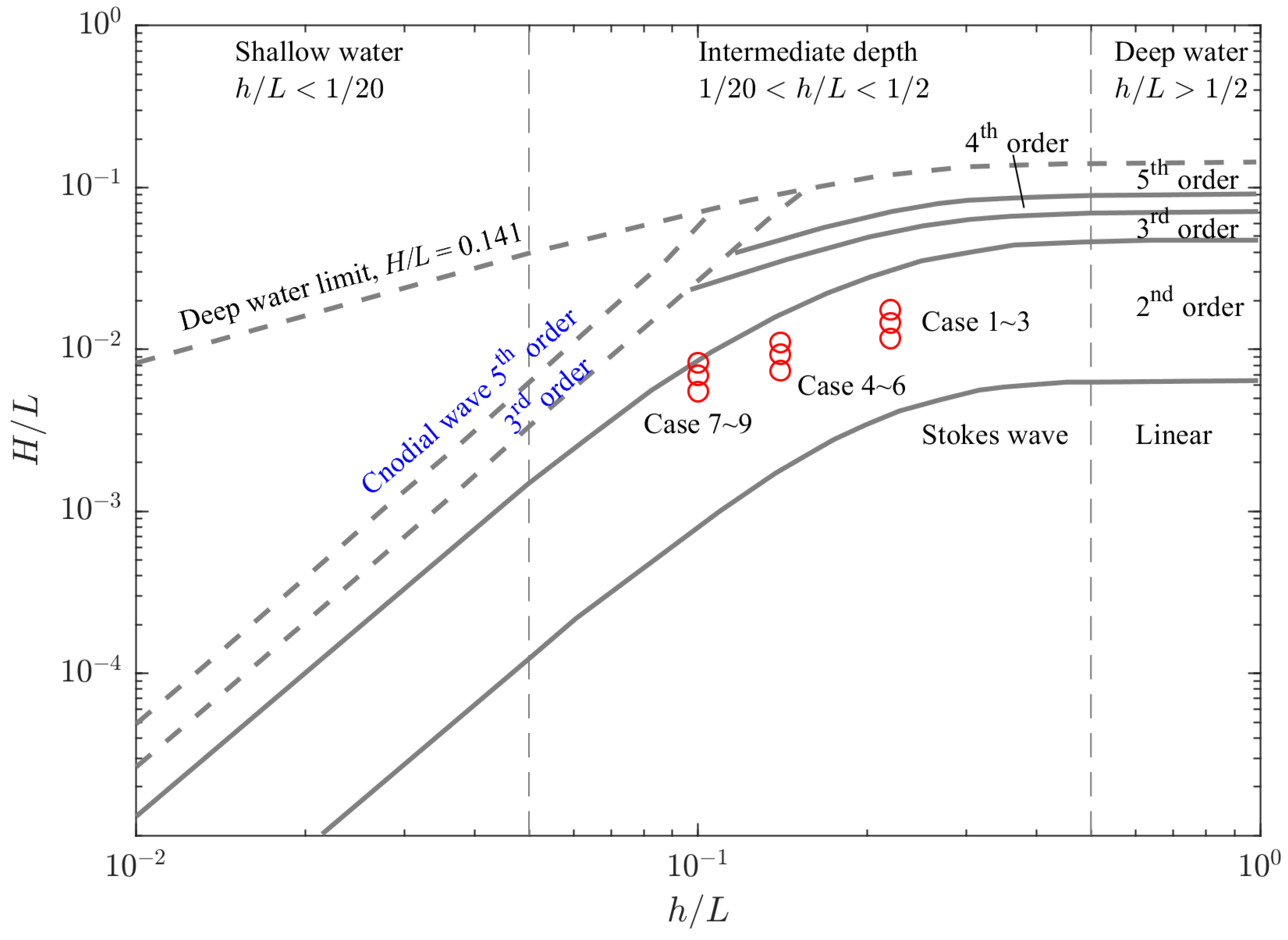
| Case | Water Depth h (m) | Wave Period T (s) | Wave Height H (m) | Wavelength L (m) | h/L | H/L | Wave Type |
|---|---|---|---|---|---|---|---|
| 1 | 2.28 | 5 | 0.4 | 34.3 | 0.22 | 0.0117 | second–order stokes wave |
| 2 | 2.28 | 5 | 0.5 | 34.3 | 0.22 | 0.0146 | second–order stokes wave |
| 3 | 2.28 | 5 | 0.6 | 34.3 | 0.22 | 0.0175 | second–order stokes wave |
| 4 | 2.28 | 7 | 0.4 | 53.9 | 0.14 | 0.0074 | second–order stokes wave |
| 5 | 2.28 | 7 | 0.5 | 53.9 | 0.14 | 0.0093 | second–order stokes wave |
| 6 | 2.28 | 7 | 0.6 | 53.9 | 0.14 | 0.0111 | second–order stokes wave |
| 7 | 2.28 | 9 | 0.4 | 72.4 | 0.1 | 0.0055 | second–order stokes wave |
| 8 | 2.28 | 9 | 0.5 | 72.4 | 0.1 | 0.0069 | second–order stokes wave |
| 9 | 2.28 | 9 | 0.6 | 72.4 | 0.1 | 0.0083 | second–order stokes wave |
| Case | Porosity n | Shear Modulus G (Pa) | Bulk Modulus of Elasticity of the Pore Fluid K (Pa) | Permeability Coefficient ks (m/s) | |
|---|---|---|---|---|---|
| 10 | 0.35 | 0.4 | 8 × 10⁶ | 2 × 10⁷ | 10−5 |
| 11 | 0.35 | 0.4 | 8 × 10⁶ | 2 × 10⁷ | 10−4 |
| 12 | 0.35 | 0.4 | 8 × 10⁶ | 2 × 10⁷ | 10−3 |
| 13 | 0.35 | 0.4 | 8 × 10⁵ | 2 × 10⁷ | 10−4 |
| 14 | 0.35 | 0.4 | 8 × 10⁷ | 2 × 10⁷ | 10−4 |
| 15 | 0.35 | 0.4 | 8 × 10⁶ | 5 × 10⁶ | 10−4 |
| 16 | 0.35 | 0.4 | 8 × 10⁶ | 2 × 10⁹ | 10−4 |
Disclaimer/Publisher’s Note: The statements, opinions and data contained in all publications are solely those of the individual author(s) and contributor(s) and not of MDPI and/or the editor(s). MDPI and/or the editor(s) disclaim responsibility for any injury to people or property resulting from any ideas, methods, instructions or products referred to in the content. |
© 2024 by the authors. Licensee MDPI, Basel, Switzerland. This article is an open access article distributed under the terms and conditions of the Creative Commons Attribution (CC BY) license (https://creativecommons.org/licenses/by/4.0/).
Share and Cite
Chen, N.; Tong, L.; Zhang, J.; Guo, Y.; Liu, B.; Zhou, Z. Wave–Induced Soil Dynamics and Shear Failure Potential around a Sandbar. J. Mar. Sci. Eng. 2024, 12, 1418. https://doi.org/10.3390/jmse12081418
Chen N, Tong L, Zhang J, Guo Y, Liu B, Zhou Z. Wave–Induced Soil Dynamics and Shear Failure Potential around a Sandbar. Journal of Marine Science and Engineering. 2024; 12(8):1418. https://doi.org/10.3390/jmse12081418
Chicago/Turabian StyleChen, Ning, Linlong Tong, Jisheng Zhang, Yakun Guo, Bo Liu, and Zhipeng Zhou. 2024. "Wave–Induced Soil Dynamics and Shear Failure Potential around a Sandbar" Journal of Marine Science and Engineering 12, no. 8: 1418. https://doi.org/10.3390/jmse12081418