Underwater Long Baseline Positioning Based on B-Spline Surface for Fitting Effective Sound Speed Table

Abstract

Due to the influence of the complex underwater environment, the sound speed constantly changes, resulting in the acoustic signal propagation trajectory being curved, which greatly affects the positioning accuracy of the underwater long baseline (LBL) system. In this paper, an improved LBL positioning method based on a B-spline surface for fitting the effective sound speed table (ESST) is proposed. Firstly, according to the underwater sound speed profile, the discrete ESST of each measurement station is constructed before the positioning test, and then, the node position of the B-spline surface is optimized by particle swarm optimization (PSO) to accurately fit the discrete ESST. Based on this, the improved LBL positioning method is constructed. In the underwater positioning test, the effective sound speed can be quickly found by measuring the time of arrival (TOA) of the acoustic signal and the target depth, and moreover, the target position parameters can be quickly and accurately estimated. The numerical simulation results show that the improved positioning method proposed in this paper can effectively improve the LBL positioning accuracy and provide the theoretical basis and the technical support for the underwater navigation and positioning.

1. Introduction

Underwater target positioning and navigation plays an important role in marine resource exploration, underwater facilities layout and marine environment measurement and so on [1,2]. With the development of marine science and technology, higher positioning accuracy has been put forward for the underwater target positioning test to meet the increasingly complex needs of marine development projects [3,4]. Therefore, the high-accuracy and fast underwater positioning method has important research significance and application value [5,6].

The positioning and navigation of aerial targets rely on the global navigation satellite system (GNSS), which is based on the electromagnetic wave. However, the attenuation of the electromagnetic wave underwater is extremely fast. Therefore, the electromagnetic wave cannot propagate over a long distance and cannot be directly used for underwater target positioning and navigation. The attenuation of the acoustic signal underwater is small, so the acoustic signal can propagate long distance. Therefore, the underwater target positioning mainly depends on the system based on the acoustic signal [7,8].

According to the baseline length, underwater positioning systems can be divided into the ultra-short baseline (USBL) system, the short baseline (SBL) system and the long baseline (LBL) system [9,10]. The length of USBL is approximately a few centimeters. The USBL system can obtain the distance and pitch angle from the target to the positioning system by measuring the phase difference and the TOA of the acoustic signal to the receiving unit, and the position parameters of the target can be obtained. The positioning accuracy of the USBL system is greatly affected by the distance, so it is not suitable for the long-distance target positioning [11,12]. The positioning method of the SBL system and the LBL system is similar. The position parameters of the target can be estimated by measuring the TOA of the acoustic signal to the receiving unit. However, the SBL system length is relatively short and is generally installed at the bottom of the ship, so the measurement range is small, and the accuracy for the long-distance positioning is poor. The baseline length of the LBL system is generally several hundred meters to several kilometers, and the LBL system is usually installed on the seabed. Due to the long length of the baseline, the LBL positioning system can achieve higher accuracy for underwater target positioning over a large measurement range. Therefore, the LBL system is widely used for underwater target navigation and positioning [13].

The main factors to affect the positioning accuracy of the LBL system include station position error, TOA measurement error and sound speed error. Due to the measurement station installed on the seabed, the station position cannot be obtained through GNSS, so it is necessary to calibrate the station in advance. The measurement ship can greatly reduce the station position error by measuring the station in a large range and multiple times, so the impact of the station position error on the positioning accuracy is relatively small. Before the underwater target positioning test, the time calibration of the LBL system can be carried out, so the TOA error can be ignored. Due to the influence of the complex underwater environment, the underwater sound speed constantly changes with the space, resulting in a curved propagation trajectory of the acoustic signal and a large positioning error. Therefore, it is necessary to study the high-accuracy positioning method for the uncertainty of the underwater sound speed.

At present, the research on the sound speed variation mainly includes the following methods: the ray tracing method, the equivalent sound speed profile (ESSP) method [14,15] and the effective sound speed method [16,17].

The ray tracing method assumes that the sound speed is a vertically layered model, that is, the change in the sound speed in the horizontal direction can be ignored, and the sound speed only varies with the depth. According to the different processing methods for the sound speed in layers, it can be divided into the constant sound speed gradient ray tracking method and the constant sound speed ray tracking method. The constant sound speed gradient ray tracking method assumes that the sound speed changes uniformly with the depth in each layer, and the other ray tracking method assumes that the sound speed remains unchanged in each layer. Although both of the above methods are approximations of the sound speed profile, the constant sound speed gradient ray tracking method is more in line with actual sound speed profile and is more accurate theoretically. Based on the constant sound speed gradient, the ray tracking method uses the ray equation to simulate the propagation trajectory of the acoustic signal underwater and deduces that the propagation trajectory of the acoustic signal in the layer is an arc [18,19]. The ray tracking method is theoretically rigorous and can be used to achieve high-accuracy underwater positioning. However, the ray tracking method requires a large amount of calculation and takes a long time, which does not meet the requirements for the fast positioning test [20,21].

The ESSP method simplifies the ray tracking method by converting the actual complex multi-layer sound speed profile into a one-layer sound speed profile, where the gradient within the layer is constant. The ESSP method simplifies the acoustic signal propagation trajectory to an arc, making the method faster than the constant sound speed gradient ray tracking method but with lower positioning accuracy.

The effective sound speed is the ratio of the linear distance between two underwater positions and the TOA of the acoustic signal. In the case of the determined sound speed profile, the effective sound speed is an implicit function of the two underwater positions. The construction of the effective sound speed equates the curved propagation trajectory to a straight line. Before the positioning test, the sound speed profile is measured, and the ESST is established. The horizontal distance between the measurement station and the target can be calculated according to the TOA data and the target depth, so as to obtain the optimal estimation of the target position parameters. Since the ESST is constructed before the test, the target position parameters can be quickly estimated in the positioning test. In addition, the positioning accuracy is equivalent to that of the ray tracking method. Therefore, the effective sound speed method can meet the requirements for high accuracy and fast positioning. The key of the positioning method based on the effective sound speed is how to obtain the effective sound speed quickly and accurately in the positioning test. For the USBL underwater positioning system, Sun et al. used the genetic algorithm (GA) to extract the sparse effective sound speed table (S-ESST) from the ESST and then searched the optimal effective sound speed from the S-ESST to achieve high-accuracy underwater positioning [22]. Zhang et al. used the constant gradient sound speed profile to approximate the actual sound speed profile, in order to simplify the calculation process and achieve the fast-positioning result [23]. In addition, Haung et al. assumed that the measurement stations are on the same horizontal plane, and the target depth is known, and fitted the effective sound speed as a cubic polynomial related to the horizontal distance [24]. Although the above processing methods can quickly estimate the target position parameters, the fitting accuracy for the effective sound speed is limited, so the improvement of the positioning accuracy is limited.

To sum up, in order to eliminate the influence of the sound speed variation on the positioning accuracy of the underwater LBL system, an improved high-accuracy positioning method for LBL based on a B-spline surface for fitting ESST is proposed in this paper. The B-spline surface is used to fit the discrete ESST in this method, and the TOA data are converted into the effective sound speed. The improved method simplifies the positioning process and improves the positioning accuracy. Firstly, based on the theory of the constant sound speed gradient ray tracking and the sound speed profile, the effective sound speed is converted into an implicit function related to the horizontal distance and the target depth, and then, the discrete ESST of each measurement station can be constructed. Due to the fact that the discrete ESST cannot be directly used to solve the positioning model, and the large amount of data in the ESST is not conducive to storage, the B-spline surface is used to fit the discrete ESST in this paper, and the continuous effective sound speed data can be obtained. In addition, the effective sound speed is converted into a function of the node position and the coefficient matrix of B-spline, which greatly reduces the amount of ESST data. The main factor to affect the fitting accuracy for B-spline surface is the node position. Therefore, this paper uses PSO to obtain the optimal node position and improve the fitting accuracy. Finally, according to the continuous effective sound speed surface, the improved LBL underwater positioning model is constructed. Based on the TOA data and the target depth, the improved LBL positioning model can quickly and accurately estimate the target position parameters. Therefore, the improved model can meet the high accuracy and fast underwater positioning requirements.

The structure of the rest of this paper is as follows: The traditional LBL positioning model and the construction method of the ESST based on the ray tracking theory are introduced in Section 2. Section 3 constructs the continuous effective sound speed data by using a B-spline surface for fitting the discrete ESST, and PSO is adopted to obtain the optimal node position. Based on this, the high-accuracy and fast LBL positioning model is constructed. The numerical simulation is conducted in Section 4. Compared with the traditional underwater LBL positioning model, the proposed LBL positioning model based on B-spline surface fitting ESST has the advantages of fast positioning speed and high positioning accuracy. Finally, the conclusions are drawn in Section 5.

2. Basic Principles

2.1. LBL Positioning Model

As shown in Figure 1, the LBL system consists of multiple stations, which are arranged on the seabed. One point on the water surface is selected as the origin $\mathit{O}(0,0,0)$ of the coordinate in the measurement range of the LBL positioning system. A coordinate system is constructed, where x, y and z point toward the east, north and the center of the Earth, respectively.

The time of the target and the LBL system is synchronized. In the underwater positioning test, the underwater target $\mathit{X}$ emits the acoustic signal, and the measurement station ${\mathit{S}}_j,j=1,\dots ,m$ receives the acoustic signal. The TOA data $t_j$ can be obtained by recording the emission and reception time of the acoustic signal. The straight distance $R_j$ from the target $\mathit{X}$ to the measurement station ${\mathit{S}}_j$ can be calculated by using the formula:

$$R_j=c·t_j,$$

(1)

where c is the underwater sound speed.

According to the geometric relationship between the target and the station, the LBL positioning model can be constructed:

$$R_j=\sqrt{{(x-x_j)}^2+{(y-y_j)}^2+{(z-z_j)}^2},$$

(2)

where $\mathit{X}=[x,y,z{]}^{\mathrm{T}}$ and ${\mathit{S}}_j=[x_j,y_j,z_j{]}^{\mathrm{T}}$.

Let

$$f_j(x,y,z)=\sqrt{{(x-x_j)}^2+{(y-y_j)}^2+{(z-z_j)}^2}-R_j.$$

(3)

The objective equation for solving the positioning model is as follows:

$$min\sum _j^m{\left(f_j\right)}^2=min\sum _j^m{(\sqrt{{(x-x_j)}^2+{(y-y_j)}^2+{(y-y_j)}^2}-R_j)}^2.$$

(4)

The Jacobian matrix of the model (3) is as follows:

$$\mathit{J}=\left(\begin{array}{ccc}\hfill {\displaystyle \frac{\left(x-x_1\right)}{R_1}}\hfill & {\displaystyle \frac{\left(y-y_1\right)}{R_1}}& {\displaystyle \frac{\left(z-z_1\right)}{R_1}}\\ \hfill {\displaystyle \frac{\left(x-x_2\right)}{R_2}}\hfill & {\displaystyle \frac{\left(y-y_2\right)}{R_2}}& {\displaystyle \frac{\left(z-z_2\right)}{R_2}}\\ \hfill \hfill & \cdots & \\ \hfill {\displaystyle \frac{\left(x-x_m\right)}{R_m}}\hfill & {\displaystyle \frac{\left(y-y_m\right)}{R_m}}& {\displaystyle \frac{\left(z-z_m\right)}{R_m}}\end{array}\right)$$

(5)

The optimal estimation $\widehat{\mathit{X}}={(\widehat{x},\widehat{y},\widehat{z})}^{\mathrm{T}}$ of the target position parameters can be obtained by using the nonlinear iterative method.

According to the positioning model (2), the main factors to affect the target positioning accuracy are the station position error, the TOA error and the sound speed error. The station position error and the TOA error can be calibrated before the underwater positioning test; thus, the sound speed error is the main factor to affect the target positioning accuracy. Due to the influence of the underwater environment, the underwater sound speed varies at different positions. The traditional model simplifies the underwater sound speed to the constant value and calculates the average sound speed $\overline{c}$ by measuring the underwater sound speed profile. The average sound speed $\overline{c}$ is used as the underwater sound speed and is substituted into (1) to calculate the straight distance. The traditional LBL positioning model is as follows:

$$\overline{c}·t_j=\sqrt{{(x-x_j)}^2+{(y-y_j)}^2+{(z-z_j)}^2}.$$

(6)

As Figure 2 shows, due to the variation in the underwater sound speed, the propagation trajectory of the acoustic signal is curved, resulting in a large positioning error of the traditional model. Therefore, it is necessary to consider the sound speed variation.

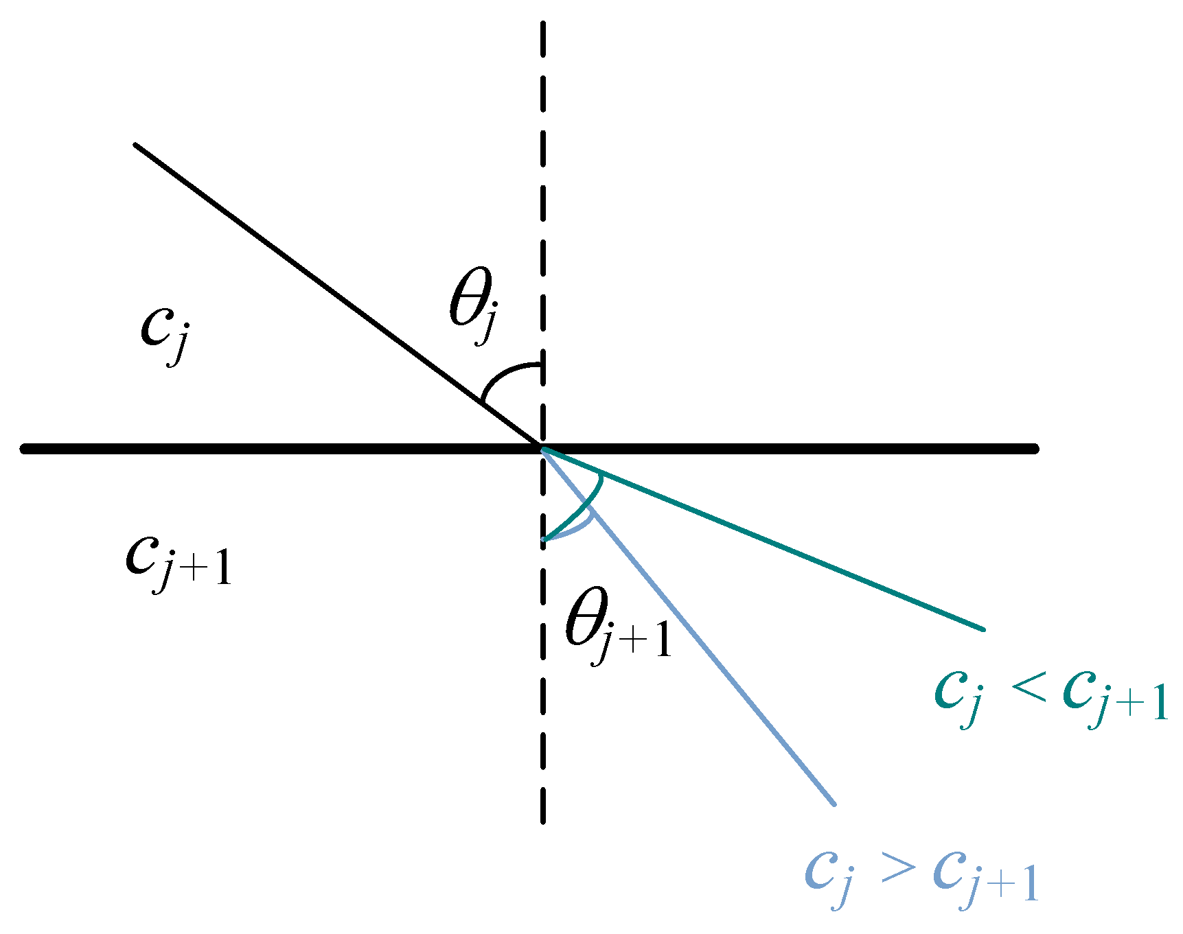
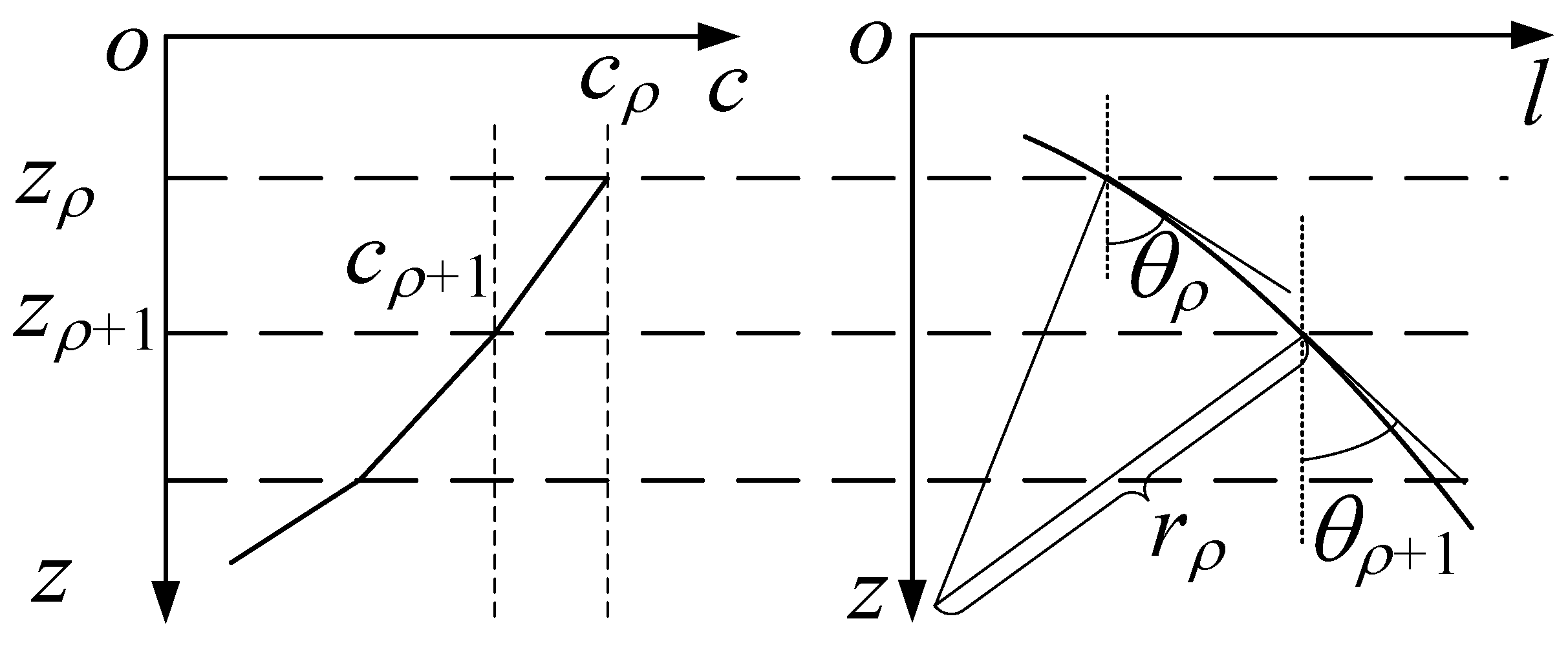
2.2. Construction of ESST Based on Ray Tracking

In open water, the variation in sound speed is 2–3 orders of magnitude higher in the vertical direction than in the horizontal direction. When the test area is small, the sound speed changes less in the horizontal direction. Therefore, it can be assumed that the sound speed remains constant horizontally and only varies with depth.

As shown in Figure 3, the change in the sound speed causes the acoustic signal to refract along the propagation direction, making the actual propagation path of the acoustic signal a continuous curve. The key to improve the LBL system positioning accuracy is to effectively eliminate the influence of the curved propagation trajectory. Based on the sound speed profile, ray tracking is an effective method to eliminate the influence of sound trajectory bending.

As shown in Figure 3, the incidence angle of the sound trajectory at point A is denoted by $\theta$. The horizontal propagation distance $dl$ can be obtained by intercepting a sufficiently small sound trajectory at A point:

$$dl=tan\theta dz.$$

(7)

Further, the following can be obtained:

$$dl={\displaystyle \frac{sin\theta }{\sqrt{1-{sin}^2\theta }}}dz={\displaystyle \frac{c\left(z\right)sin{\theta }_0}{\sqrt{c_0^2-c{\left(z\right)}^2{sin}^2{\theta }_0}}}dz,$$

(8)

where ${\theta }_0$ is the initial incidence angle.

Assume that the emission position of the acoustic signal is ${\mathit{X}}_1={[x_1,y_1,z_1]}^{\mathrm{T}}$, and the reception position is ${\mathit{X}}_2={[x_2,y_2,z_2]}^{\mathrm{T}}$. The starting and ending positions of the sound trajectory are ${\mathit{X}}_1,{\mathit{X}}_2$.

By integrating (8), the horizontal distance of the sound trajectory can be obtained:

$$l={\int }_{z_1}^{z_2}{\displaystyle \frac{c\left(z\right)sin{\theta }_0}{\sqrt{c_0^2-c{\left(z\right)}^2{sin}^2{\theta }_0}}}dz,$$

(9)

where $z_1,z_2$ are the depths of the starting and ending points of the sound trajectory.

Similarly, $dR$ can be obtained:

$$dR={\displaystyle \frac{dz}{cos\theta }}={\displaystyle \frac{c_0}{\sqrt{c_0^2-c{\left(z\right)}^2{sin}^2{\theta }_0}}}dz.$$

(10)

The acoustic signal propagation distance R can be obtained:

$$R={\int }_{z_1}^{z_2}{\displaystyle \frac{c_0}{\sqrt{c_0^2-c{\left(z\right)}^2{sin}^2{\theta }_0}}}dz.$$

(11)

According to (11), the acoustic signal propagation time t can be obtained:

$$t=\int {\displaystyle \frac{dR}{c}}={\int }_{z_1}^{z_2}{\displaystyle \frac{c_0}{c\left(z\right)\sqrt{c_0^2-c{\left(z\right)}^2{sin}^2{\theta }_0}}}dz.$$

(12)

Before the underwater positioning test, it is necessary to obtain the underwater sound speed profile, which can be measured directly or calculated by the empirical formula. As the sound speed profile is discrete, the constant sound speed gradient ray tracking method is adopted in this paper.

As shown in Figure 4, assuming the depth range of the ρ-th layer is $\left[z_{\rho },z_{\rho +1}\right]$, the underwater sound speed range is $\left[c_{\rho },c_{\rho +1}\right]$, and the incident angle of the sound trajectory is ${\theta }_{\rho },\rho =1,\dots ,\Gamma$. According to Snell’s law of ray acoustics, the sound speed $c_{\rho }$ and the incidence angle ${\theta }_{\rho }$ are satisfied:

$${\displaystyle \frac{sin{\theta }_1}{c_1}}=\cdots ={\displaystyle \frac{sin{\theta }_{\Gamma }}{c_{\Gamma }}}=p,$$

(13)

where p is an unknown constant, and the incidence angle ${\theta }_{\rho }$ is the angle between the propagation direction of the sound trajectory in depth $z_{\rho }$ and the vertical direction.

By differentiating both sides of the (13), we can obtain the following:

$${\displaystyle \frac{d\theta }{dR}}={\displaystyle \frac{sin\theta }{c}}{\displaystyle \frac{dc}{dz}}.$$

(14)

Assume the sound speed varies in a constant gradient $g_{\rho }$ in layers. According to (14), the trajectory of the acoustic signal in the ρ-th layer is an arc, and the radius $r_{\rho }$ of the arc is as follows:

$$r_{\rho }=\left|{\displaystyle \frac{1}{p{g}_{\rho }}}\right|.$$

(15)

As shown in Figure 5, the horizontal propagation distance $l_{\rho }$ of acoustic signal in the ρ-th layer is as follows:

$$l_{\rho }=\left|r_{\rho }\left(cos{\theta }_{\rho }-cos{\theta }_{\rho +1}\right)\right|={\displaystyle \frac{1}{p{g}_{\rho }}}\left(cos{\theta }_{\rho }-cos{\theta }_{\rho +1}\right).$$

(16)

Thus, Equation (9) can be simplified as follows:

$$l=\sum {\displaystyle \frac{1}{p{g}_{\rho }}}\left(cos{\theta }_{\rho }-cos{\theta }_{\rho +1}\right).$$

(17)

Similarly, the acoustic signal propagation distance $R_{\rho }$ in the ρ-th layer can be obtained:

$$R_{\rho }=\left|r_{\rho }\left({\theta }_{\rho +1}-{\theta }_{\rho }\right)\right|=r_{\rho }\left({\theta }_{\rho +1}-{\theta }_{\rho }\right).$$

(18)

Furthermore, the Equation (11) can be simplified as follows:

$$R=\sum r_{\rho }\left({\theta }_{\rho +1}-{\theta }_{\rho }\right).$$

(19)

Let the propagation time of the acoustic signal along the circular arc in the ρ-th layer be $t_{\rho }$. According to $dt=dR/c$, we can obtain the following:

$$t_{\rho }={\int }_{sin{\theta }_{\rho }/p}^{sin{\theta }_{\rho +1}/p}{\displaystyle \frac{r_{\rho }p}{c\sqrt{1-p^2{c}^2}}}dc.$$

(20)

Furthermore, let

$$\zeta =pc,$$

(21)

where the range of $\zeta$ is $\left[sin{\theta }_{\rho },sin{\theta }_{\rho +1}\right]$.

The Equation (20) can be written as follows:

$$t_{\rho }={\int }_{sin{\theta }_{\rho }}^{sin{\theta }_{\rho +1}}{\displaystyle \frac{r_{\rho }p}{\zeta \sqrt{1-{\zeta }^2}}}d\zeta ={\displaystyle \frac{1}{g_{\rho }}}(ln\left(tan\left({\displaystyle \frac{{\theta }_{\rho +1}}{2}}\right)\right)-ln\left(tan\left({\displaystyle \frac{{\theta }_{\rho }}{2}}\right)\right)).$$

(22)

The acoustic signal propagation time can be simplified as follows:

$$t=\sum {\displaystyle \frac{1}{g_{\rho }}}(ln(tan\left({\displaystyle \frac{{\theta }_{\rho +1}}{2}}\right))-ln(tan\left({\displaystyle \frac{{\theta }_{\rho }}{2}}\right))).$$

(23)

The definition of the effective sound speed is the ratio of the straight distance between the two ends of the sound trajectory to the propagation time:

$$c={\displaystyle \frac{R_s}{t}}={\displaystyle \frac{\sqrt{{(\sum \frac{1}{p{g}_{\rho }}(cos{\theta }_{\rho }-cos{\theta }_{\rho +1}))}^2+({\mathrm{z}}_1-z_2{)}^2}}{\sum \frac{1}{g_{\rho }}(ln(tan\left(\frac{{\theta }_{\rho +1}}{2}\right))-ln(tan\left(\frac{{\theta }_{\rho }}{2}\right)))}}.$$

(24)

When the sound speed profile, the station position and the target position are known, the initial incident angle of sound trajectory can be calculated, and then, the effective sound speed can be calculated according to (13) and (24). Therefore, when the sound speed profile is determined, the effective sound speed is a complex implicit function related to the horizontal distance and the target depth. Before the underwater positioning test, the ESST can be constructed by setting equidistant sampling positions. However, as the ESST is discrete, it cannot be directly used in the underwater positioning test. Therefore, the B-spline surface is used in this paper to fit the discrete effective sound speed with high accuracy and construct a continuous effective sound speed surface, so as to realize fast and high-accuracy positioning.

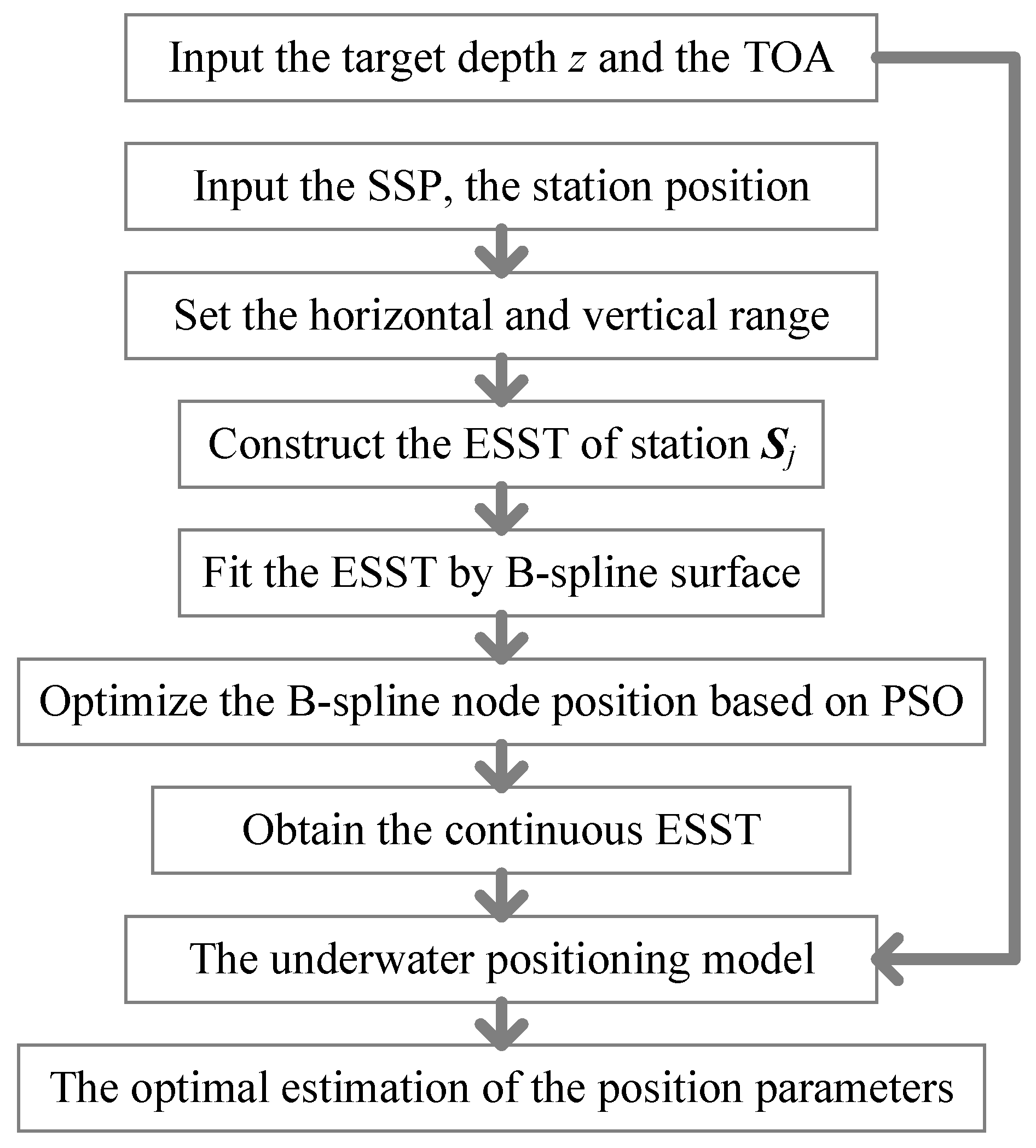
3. LBL Positioning Method Based on B-Spline Surface for Fitting ESST

3.1. B-Spline Surface Fitting ESST

The key to fitting the discrete ESST is to find a simple function that approximates the scattered effective sound speed with high accuracy. Because the B-spline function can fit discrete data well, the B-spline surface is used to fit the discrete ESST in this paper.

$U:a=T_0<T_1<\cdots <T_{N-1}<T_N=b$ is the division of the interval $\left[a,b\right]$, let

$$w_{\iota ,P+1}\left(\xi \right)=\left(\xi -T_{\iota }\right)\left(\xi -T_{\iota +1}\right)\cdots \left(\xi -T_{\iota +P+1}\right),$$

(25)

where $T_1,\dots ,T_{N-1}$ is the inner node position.

The $\iota \text{-}th$ function of $P+1$ order B-spline is as follows:

$$B_{\iota ,p+1}\left(\xi \right)=\left(T_{\iota +P+1}-T_{\iota }\right)\sum _{k=\iota }^{\iota +n+1}{\displaystyle \frac{{\left(T_k-\xi \right)}_{+}^P}{w_{\iota ,P+1}^{\prime }\left(T_k\right)}}.$$

(26)

The curve constructed by the $P+1$ order B-spline is follows:

$${\mathit{S}}_{curve}\left(\xi \right)=\sum _{\iota =-P}^{N-1}{B}_{\iota ,P+1}\left(\xi \right)b_{\iota }.$$

(27)

Similar to the curve construction method, the surface constructed by the B-spline surface is as follows:

$${\mathit{S}}_{surface}({\xi }_1,{\xi }_2)=\sum _{\iota =-P_1}^{N_1-1}\sum _{\phi =-P_2}^{N_2-1}{b}_{\iota ,\phi }{B}_{\iota ,p_1+1}\left({\xi }_1\right)B_{\phi ,p_2+1}\left({\xi }_2\right),$$

(28)

where $B_{\iota ,p_1+1}\left({\xi }_1\right)$ and $B_{\phi ,p_2+1}\left({\xi }_2\right)$ are the $P_1+1$ order and $P_2+1$ order spline basic functions for ${\xi }_1$ and ${\xi }_2$, respectively.

The B-spline surface is used to fit the discrete ESST in this paper, and the effective sound speed is represented as a complex implicit function related to the horizontal distance and the target depth. Assuming the horizontal distance range is $[L_b,L_e]$ and the target depth range is $[Z_b,Z_e]$, the ESST $\mathit{\chi }$ of the measurement station can be fitted:

$$\mathit{\chi }(l,z)=\mathit{S}(l,z)+\mathit{e}.$$

(29)

Let

$$\begin{array}{c}\begin{array}{c}{\mathit{B}}_z\left({\mathit{T}}^z\right)={\left[B_{\iota ,p+1}\left({\mathit{T}}^z,t_{\mu }\right)\right]}_{\begin{array}{c}\mu =1,\dots ,M_1\\ \iota =-p_1,\dots ,N_1-1\end{array}}\hfill \\ {\mathit{B}}_l\left({\mathit{T}}^l\right)={\left[B_{\phi ,p+1}\left({\mathit{T}}^l,l_{\nu }\right)\right]}_{\begin{array}{c}\nu =1,\dots ,M_2\\ \phi =-p_2,\dots ,N_2-1\end{array}}\hfill \\ \mathit{\beta }={\left[b_{\iota \phi }\right]}_{\begin{array}{c}i=-p_1,\dots ,N_1-1\\ \phi =-p_2,\dots ,N_2-1\end{array}}\hfill \\ \mathit{\chi }={\left[c_{\mu \nu }\right]}_{\begin{array}{c}\mu =1,\dots ,M_1\\ \nu =1,\dots ,M_2\end{array}}\hfill \\ \mathit{e}={\left[e\right]}_{\begin{array}{c}\mu =1,\dots ,M_1\\ \nu =1,\dots ,M_2\end{array}}.\hfill \end{array}\hfill \end{array}$$

(30)

The Equation (29) can be written in vector form:

$$\mathit{\chi }=\mathit{S}(l,z)+\mathit{e}={\mathit{B}}_l\mathit{\beta }{\mathit{B}}_z^{\mathrm{T}}+\mathit{e}.$$

(31)

The fitting accuracy of the B-spline surface is directly affected by the node position. Therefore, the optimal node position is the key to the underwater fast and high-accuracy positioning test. The optimization problem of node position can be written as follows:

$$min\mathit{F}({\mathit{T}}^z,{\mathit{T}}^l,\mathit{\beta })=min{∥\mathit{e}∥}^2=min{∥\mathit{\chi }-{\mathit{B}}_l\mathit{\beta }{\mathit{B}}_z^{\mathrm{T}}∥}^2.$$

(32)

The solution space of the optimization problem (32) is $((N_1+P_1)(N_2+P_2)+N_1+N_2-2)$-dimensional [25].

$\widehat{\mathit{\beta }}$ is the estimation of the coefficient matrix $\mathit{\beta }$; $\widehat{\mathit{\beta }}$ can be obtained according to the least square algorithm:

$$\widehat{\mathit{\beta }}={\left({\mathit{B}}_l^{\mathrm{T}}{\mathit{B}}_l\right)}^{-1}{\mathit{B}}_l^{\mathrm{T}}\mathit{\chi }{\mathit{B}}_z{\left({\mathit{B}}_z^{\mathrm{T}}{\mathit{B}}_z\right)}^{-1}.$$

(33)

Let

$$\begin{array}{c}\begin{array}{c}{\mathit{E}}^l={\mathit{B}}_l{\left({\mathit{B}}_l^{\mathrm{T}}{\mathit{B}}_l\right)}^{-1}{\mathit{B}}_l^{\mathrm{T}}\hfill \\ {\mathit{E}}^z={\mathit{B}}_z{\left({\mathit{B}}_z^{\mathrm{T}}{\mathit{B}}_z\right)}^{-1}{\mathit{B}}_z^{\mathrm{T}}.\hfill \end{array}\hfill \end{array}$$

(34)

Theorems 1 and 2 prove that the optimization problem (32) is equivalent to the optimization problem (35):

$$min\mathit{G}({\mathit{T}}^l,{\mathit{T}}^z)=min{∥\mathit{\chi }-{\mathit{E}}^l\mathit{\chi }{\left({\mathit{E}}^z\right)}^{\mathrm{T}}∥}^2.$$

(35)

Theorem 1. 

The minimum value of optimization problem (32) is equal to optimization problem (35):

$$min\mathit{F}({\mathit{T}}^l,{\mathit{T}}^z,\mathit{\beta })=min\mathit{G}({\mathit{T}}^l,{\mathit{T}}^z).$$

(36)

Theorem 2. 

If ${\mathit{T}}^l,{\mathit{T}}^z,\widehat{\mathit{\beta }}$ minimizes the optimization problem (32), then ${\mathit{T}}^l,{\mathit{T}}^z$ is also the optimal solution of (35); conversely, if ${\mathit{T}}^l,{\mathit{T}}^z$ minimizes the optimization problem (35), let $\widehat{\mathit{\beta }}={\left({\mathit{B}}_l^{\mathrm{T}}{\mathit{B}}_l\right)}^{-1}{\mathit{B}}_l^{\mathrm{T}}\mathit{\chi }{\mathit{B}}_z{\left({\mathit{B}}_z^{\mathrm{T}}{\mathit{B}}_z\right)}^{-1}$, then ${\mathit{T}}^l,{\mathit{T}}^z,\widehat{\mathit{\beta }}$ is also the optimal solution of (32).

The proofs of Theorems 1 and 2 are provided in the Appendix A.

The problem (35) only involves the node position optimization, with the solution space being $(N_1+N_2-2)$-dimensional. Therefore, the effective sound speed surface $\mathit{c}(l,z)$ with minimum fitting error can be obtained only by optimizing the node position. Due to the large number of local optima in the optimization problem of the node position, traditional nonlinear iterative methods are prone to fall into the local minimum, while the intelligent optimization methods have a simple structure and large scale convergence. Therefore, particle swarm optimization (PSO) is used to obtain the optimal node position in this paper.

3.2. Node Position Optimization Based on PSO

PSO is an intelligence algorithm proposed by Eberhart and Kennedy, inspired by the biologic swarm movement model. Similar to the genetic algorithm, PSO is an iterative optimization algorithm. The PSO algorithm does not use the competitive mechanism of the group to iteratively find the optimal solution but uses the cooperative mechanism of the group solution to iteratively find the optimal solution. Due to its simple implementation and fast convergence speed, PSO has been widely used in many fields such as function optimization, image processing, geodetic survey and so on.

PSO simulates the flight behavior of particles in the solution space, utilizing individual historical experience and group information to search and optimize solutions to optimization problems. In the PSO, each particle is represented as a node vector with its own position and velocity. The position of the node vector represents a solution in the search space, while its velocity determines the direction and distance of the particle to the next position. Each particle updates the position and velocity based on its historical best position and the global best position.

${\mathit{Pb}}_{\eta }^{\kappa }$ and ${\mathit{Gb}}_g^{\kappa }$ are the historical optimal position of the $\eta \text{-}th$ node vector and all node vectors in the $\kappa \text{-}th$ iteration, respectively. ${\mathit{T}}_{\eta }^{\kappa }$ and ${\mathit{v}}_{\eta }^{\kappa }$ are the position and the velocity of the $\eta \text{-}th$ node vector in the $\kappa \text{-}th$ iteration, respectively. The iterative equation for optimizing node position using the PSO is as follows:

$$\begin{array}{c}{\mathit{v}}_{\eta }^{\kappa +1}=w{\mathit{v}}_{\eta }^{\kappa }+c_1{r}_1\left({\mathit{Pb}}_{\eta }^{\kappa }-{\mathit{T}}_{\eta }^{\kappa }\right)+c_2{r}_2\left({\mathit{Gb}}_g^{\kappa }-{\mathit{T}}_{\eta }^{\kappa }\right)\\ {\mathit{T}}_{\eta }^{\kappa +1}={\mathit{T}}_{\eta }^{\kappa }+{\mathit{v}}_{\eta }^{\kappa +1},\end{array}$$

(37)

where w is the inertia weight, $c_1,c_2$ are the learning factor, and $r_1$,$r_2$ are the random number between 0 and 1.

In the iteration (37), the inertia weight w reflects the impact of the last iteration velocity on the current velocity. When the inertia weight w decreases with the iteration of the algorithm, the convergence ability of the PSO will be significantly improved. Therefore, the PSO based on Gaussian decreasing inertia weight is adopted in this paper, and the adjusted inertia weight is as follows:

$$w\left(\kappa \right)=\left(w_{max}-w_{min}\right)e^{-{\displaystyle \frac{{\kappa }^2}{{\left(E_t\times ite{r}_{max}\right)}^2}}}+w_{min},$$

(38)

where $E_t$ and $ite{r}_{max}$ are the expansion constant and the maximum iteration number, respectively.

The node position iterates in the specified range. If the node position exceeds the specified range in the iteration, the boundary position is taken as the node position. In the process of solving the optimal node position, the PSO cannot obtain the optimal value at one time. Through several iterations, the optimal node position is finally obtained.

3.3. Improved LBL Positioning Method

Due to the fact that the LBL system measurement data are the TOA of the acoustic signal and the TOA data cannot be directly used to estimate the underwater target position parameters, it is necessary to convert the TOA data into distance information.

According to (24) and (28), we can obtain the following:

$$\begin{array}{c}\begin{array}{c}c(l,z)=\sum _{\iota =-3}^{N_1-1}\sum _{\phi =-3}^{N_2-1}{b}_{\iota ,\phi }{B}_{\iota ,4}\left(l\right)B_{\phi ,4}\left(z\right)\hfill \\ c(l,z)={\displaystyle \frac{R}{t}}={\displaystyle \frac{\sqrt{l^2+{(z-z_j)}^2}}{t}},\hfill \end{array}\hfill \end{array}$$

(39)

where $z_j$ is the depth of the $j\text{-}th$ station, and z is the target depth.

The effective sound speed of measurement stations $c_{es{s}_1},\dots ,c_{es{s}_m}$ can be obtained according to (39), and then, the horizontal distance from the target to the $j\text{-}th$ measurement station can be obtained.

The target depth is measured by the depth gauge, so only the horizontal position parameters of the underwater target need to be estimated. The model for estimating the horizontal position parameters of the target is constructed as follows:

$$l_j=\sqrt{{(x-x_j)}^2+{(y-y_j)}^2},j=1,\dots ,m.$$

(40)

The optimal estimation $\widehat{x},\widehat{y}$ of $x,y$ can be obtained by the nonlinear iterative method:

$$(\widehat{x},\widehat{y})=argmin\sum _j^m{(\sqrt{{(x-x_j)}^2+{(y-y_j)}^2}-l_j)}^2.$$

(41)

Combined with the target depth, the optimal estimation $\widehat{\mathit{X}}={(\widehat{x},\widehat{y},\widehat{z})}^{\mathrm{T}}$ of the underwater target’s position can be obtained.

The underwater positioning process of the LBL system based on the B-spline surface fitting ESST is shown in Figure 6.

4. Numerical Simulation

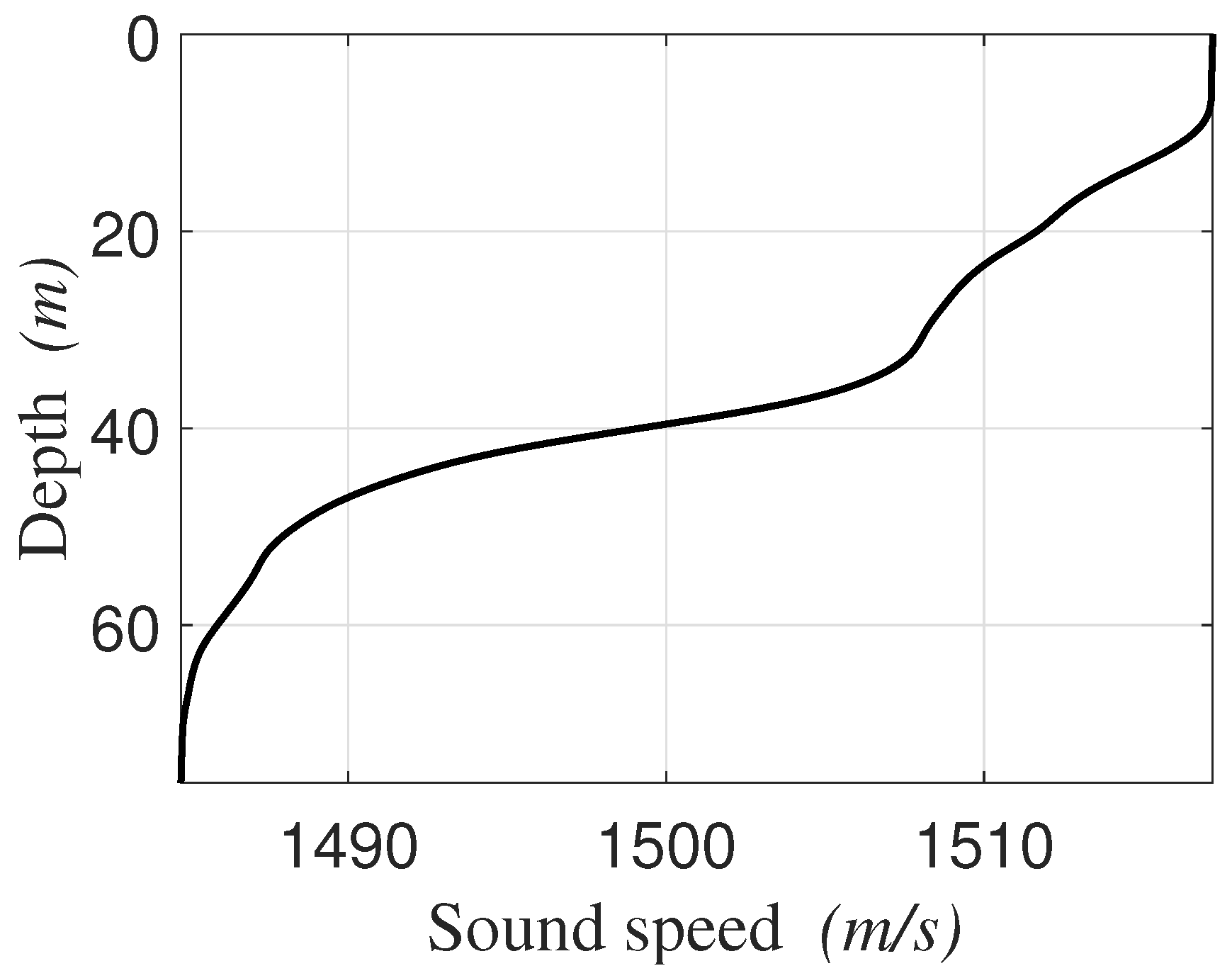
4.1. Scenario Design

In order to verify the effectiveness of the high-accuracy underwater target positioning method proposed in this paper, a numerical simulation for the underwater LBL positioning test is constructed.

As shown in Figure 7, the target moves within the measurement range of the LBL system, and 5 LBL stations are installed on the seabed. The time of the target is aligned with the LBL system. In the positioning test, the acoustic signal is emitted by the target periodically, and the LBL system receives the acoustic signal. Therefore, the TOA data can be obtained. In addition, the depth gauge is installed on the target to obtain the target depth.

The sound speed profile used in the simulation is shown in Figure 8. The TOA data can be obtained according to the position of the underwater target and the LBL station. In the simulation, it is assumed that the random error of the measurement sound speed is ${\sigma }_c=0.3$ m/s, the random error of the TOA data is ${\sigma }_t=100$ us, the random error of the station position is ${\sigma }_S=0.1$ m, and the random error of the target depth is ${\sigma }_z=0.1$ m. The random error is added to the true value to obtain the simulation measurement data.

4.2. Simulation Results

According to the sound speed profile and the position of the measurement station, the measurement points are evenly selected at an interval of $0.5$ m in the horizontal and vertical directions, and the ESST is constructed before the underwater positioning test. Taking the measurement stations ${\mathit{S}}_1$ and ${\mathit{S}}_3$ as an example, the discrete ESSTs constructed are shown in Figure 9 and Figure 10. It can be seen that the ESST of each station is also different.

Assuming that the node number in both the horizontal and depth directions is 10, the initial node position is uniformly selected within the range. The parameters $P_1$ and $P_2$ are both 3, and the surface (28) is called a bicubic B-spline surface. According to the process shown in Figure 6, the optimal node position of each measurement station can be obtained. The node position iteration in the PSO process of ${\mathit{S}}_1$ station is shown in Figure 11.

The initial spline node position and the optimal node position in the horizontal and depth directions of all measurement stations are shown in

Table 1. The optimal node position of l direction.

	${\mathit{T}}_{\mathit{l}1}$ (m)	${\mathit{T}}_{\mathit{l}2}$ (m)	${\mathit{T}}_{\mathit{l}3}$ (m)	${\mathit{T}}_{\mathit{l}4}$ (m)	${\mathit{T}}_{\mathit{l}5}$ (m)	${\mathit{T}}_{\mathit{l}6}$ (m)	${\mathit{T}}_{\mathit{l}7}$ (m)	${\mathit{T}}_{\mathit{l}8}$ (m)	${\mathit{T}}_{\mathit{l}9}$ (m)	${\mathit{T}}_{\mathit{l}10}$ (m)
$Ini$	36.3636	72.7273	109.0909	145.4545	181.8182	218.1818	254.5455	290.9091	327.2727	363.6364
$S_1$	0.0092	1.3678	101.8749	104.5886	228.5547	283.0521	285.5396	289.9352	313.4571	384.8025
$S_2$	0.0054	0.0073	5.0202	126.5374	139.6849	156.8044	180.6934	181.2321	342.4901	344.1411
$S_3$	0.0274	5.4753	81.9488	128.0599	144.4255	150.0506	194.1382	309.2122	333.4297	345.8373
$S_4$	0.0078	0.0100	1.1143	7.7296	139.3083	142.6808	172.3512	225.2021	245.1397	297.3150
$S_5$	0.0112	1.3489	70.6676	114.7475	146.9981	168.9183	232.8474	309.2341	399.9858	399.9883

and

Table 2. The optimal node position of z direction.

	${\mathit{T}}_{\mathit{z}1}$ (m)	${\mathit{T}}_{\mathit{z}2}$ (m)	${\mathit{T}}_{\mathit{z}3}$ (m)	${\mathit{T}}_{\mathit{z}4}$ (m)	${\mathit{T}}_{\mathit{z}5}$ (m)	${\mathit{T}}_{\mathit{z}6}$ (m)	${\mathit{T}}_{\mathit{z}7}$ (m)	${\mathit{T}}_{\mathit{z}8}$ (m)	${\mathit{T}}_{\mathit{z}9}$ (m)	${\mathit{T}}_{\mathit{z}10}$ (m)
$Ini$	2.7273	5.4545	8.1818	10.9091	13.6364	16.3636	19.0909	21.8182	24.5455	27.2727
$S_1$	0.0249	6.7565	13.6880	13.7749	13.8123	16.0755	18.2588	20.4489	20.4490	22.5796
$S_2$	6.6353	13.3419	13.3446	14.5304	16.6499	16.6528	19.4688	20.0315	20.3710	22.6115
$S_3$	0.0654	6.7118	13.3861	13.3939	14.4381	16.0236	18.2102	20.4504	20.4626	22.5622
$S_4$	6.6384	13.3718	13.3718	14.4618	16.0170	18.2245	20.4799	20.4801	23.5473	23.5474
$S_5$	2.0896	6.8612	13.3935	13.3935	14.4438	16.0177	18.2402	20.4521	20.4522	22.5751

, respectively.

We define the fitting accuracy $N_2$ as the 2-norm of the fitting error:

$$N_2={∥\mathit{\chi }(l,z)-\mathit{c}(l,z)∥}_2.$$

(42)

According to the node position optimization process of each station, the initial fitting accuracy and optimal fitting accuracy are shown in

Table 3. The fitting accuracy of B-spline surface.

	${\mathit{S}}_1$	${\mathit{S}}_2$	${\mathit{S}}_3$	${\mathit{S}}_4$	${\mathit{S}}_5$
The initial fitting accuracy (m/s)	0.5278	0.5276	0.5279	0.5276	0.5276
The optimal fitting accuracy (m/s)	0.1196	0.1080	0.1070	0.1111	0.1147

.

The traditional LBL positioning model (6) is $M1$, and the LBL positioning model based on the B-spline surface for fitting ESST constructed in this paper is $M2$. According to the sound speed profile, the average sound speed in $M1$ can be obtained as $\overline{c}=1500.22$ m/s. Based on the TOA data and the target depth, the target position parameters can be estimated by $M1$ and $M2$, and the estimation error in each direction are shown in Figure 12, Figure 13 and Figure 14.

The statistical results of estimation error of $M1$ and $M2$ are shown in

Table 4. The statistical error results of each model.

	$\overline{|\Delta \mathit{x}|}$ (m)	$\overline{|\Delta \mathit{y}|}$ (m)	$\overline{∥\Delta \mathit{X}∥}$ (m)
$M1$	0.2127	0.1733	0.3306
$M2$	0.0938	0.0880	0.1758

.

According to the above simulation results, we can obtain the following:

(1)

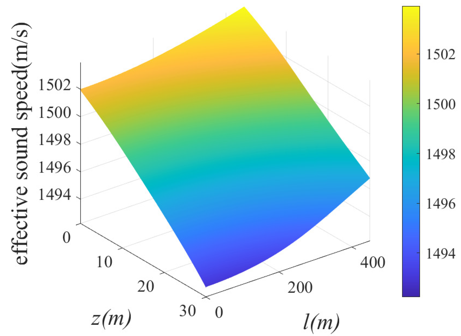
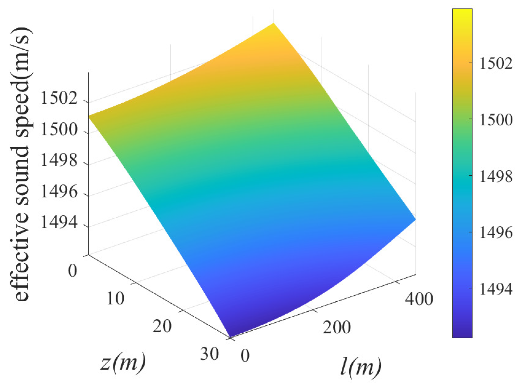
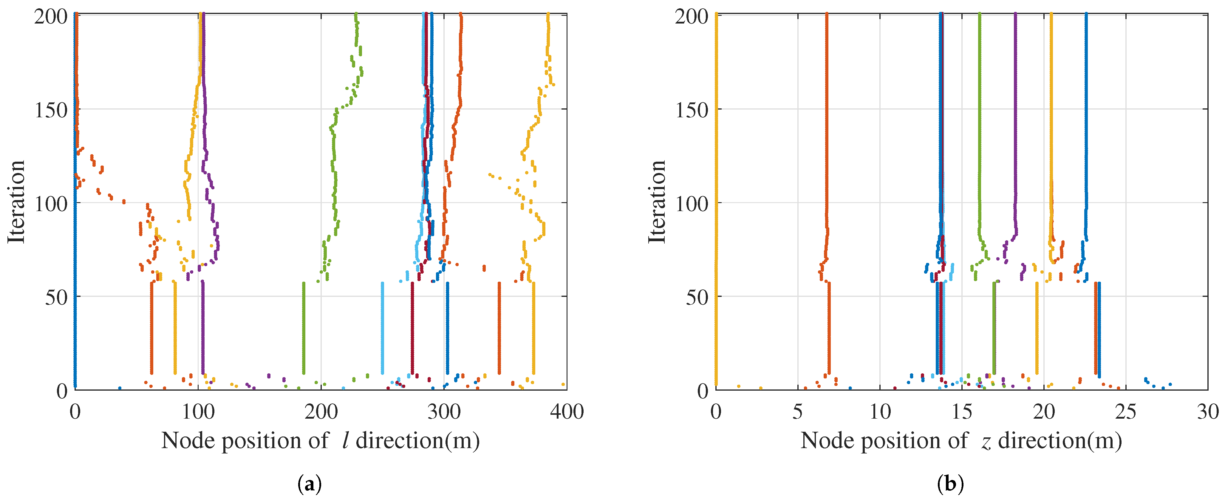
The fitting accuracy of the initial node position is limited. By optimizing the node position through the PSO, the fitting accuracy of the B-spline surface is greatly improved. Therefore, the B-spline surface fitting method based on PSO can accurately obtain the continuous ESST.

(2)

From Table 1 and Table 2, it can be seen that due to the different depth of different stations, the ESST of each station is also different, resulting in a different optimal node position of the B-spline surface;

(3)

The dimension of the discrete ESST of each measurement station is a matrix of 800 × 60. After fitting with the B-spline surface, the data volume of the fitted ESST of each measurement station is (10 × 2 + 14 × 14), and the fitted ESST is a continuous surface.

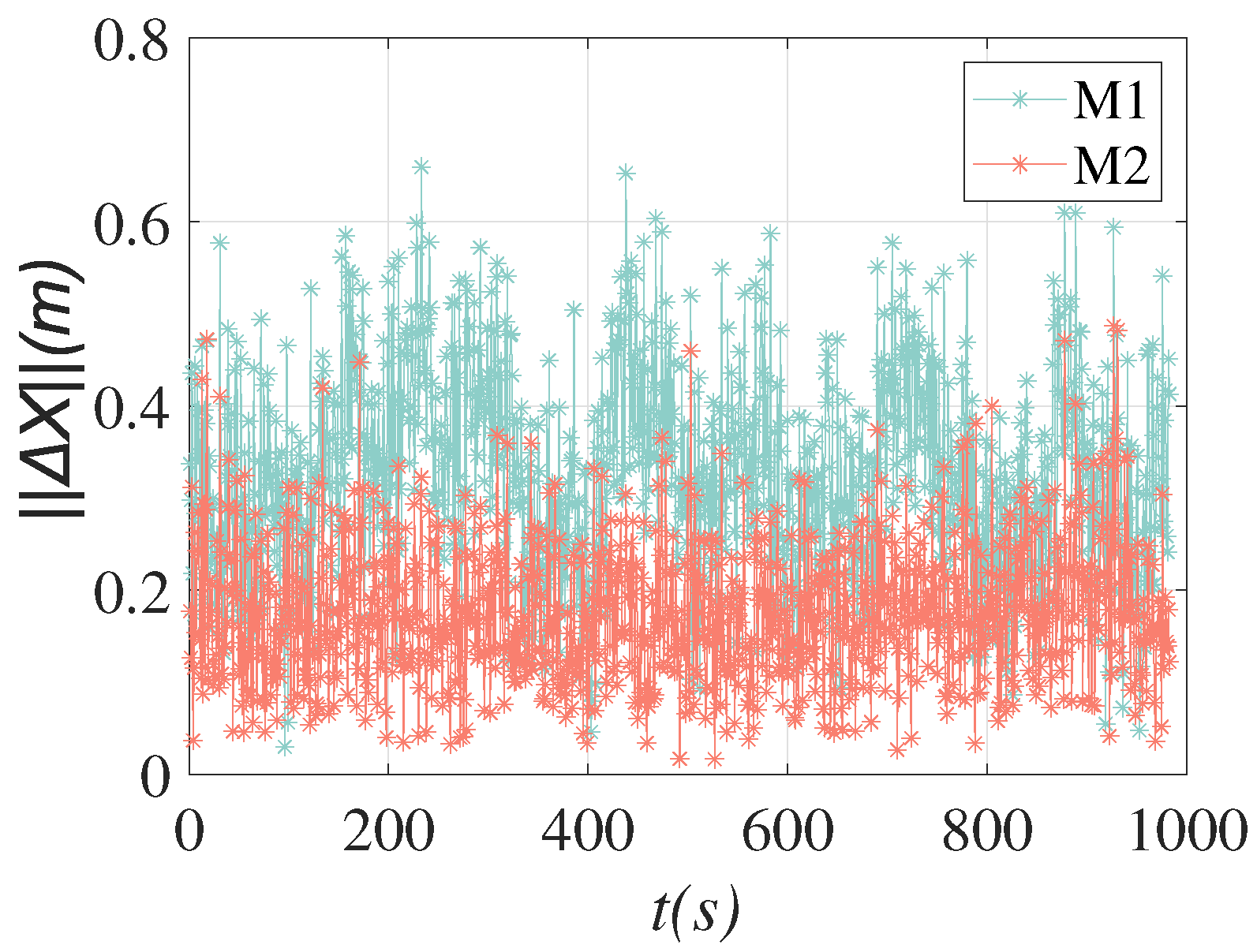
(4)

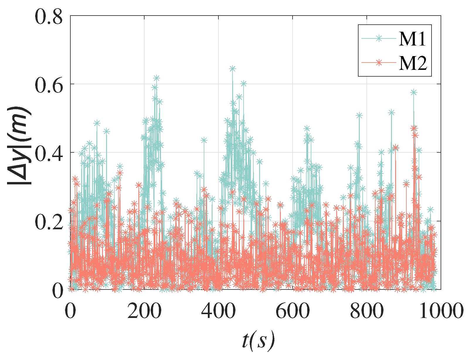
The average sound speed is taken as the underwater sound speed in the traditional LBL positioning model (6), resulting in a significant estimation error. The improved positioning model constructed in this paper is based on the theory of ray tracing and the B-spline surface fitting method. The effective sound speed is obtained based on the TOA data and the target depth, which can reduce the influence of sound speed change on the positioning accuracy. The simulation results show that the improved positioning model proposed in this paper has a smaller estimation error than the traditional positioning model.

4.3. Discussion

The vertical distribution of the underwater sound speed is a fundamental issue in underwater positioning systems. Due to the change in the sound speed, the acoustic signal refracts along the propagation direction. Therefore, many scholars are committed to improving the accuracy of underwater navigation and positioning. In this paper, we proposed an improved LBL positioning method based on a B-spline surface for fitting the ESST. The B-spline surface is used to approximate the discrete ESST, and PSO is used to optimize the node positions of the B-spline, thereby achieving an exact fit for the discrete ESST data. Based on the target depth, the improved method can effectively eliminate positioning error caused by the sound speed change and improve the underwater LBL positioning accuracy.

However, the improved LBL positioning model needs to measure the sound speed profile before the underwater positioning test and requires time to construct the ESST of each LBL system station. In addition, the depth gauge needs to be installed on the underwater target to obtain the target depth.

Therefore, the future research focus is on achieving fast and high-accuracy underwater target navigation and positioning without the depth data.

5. Conclusions

Due to the complex underwater environment, the underwater sound speed changes at different positions. The underwater sound speed is simplified to a constant value in the traditional LBL positioning method. The sound speed profile is used to obtain the average sound speed to estimate the target position parameters, resulting in a significant estimation error. In order to reduce the influence of sound speed variation on the positioning accuracy of the LBL system, the ESST is constructed based on the ray tracking theory before the underwater positioning test in this paper. Then, the effective sound speed is expressed as an implicit function of horizontal distance and target depth. Due to the fact that the ESST is discrete, it cannot be directly used for the underwater target positioning test. Therefore, the B-spline surface is used to fit the discrete ESST in this paper, and the PSO algorithm is used to optimize node position. The high-accuracy continuous surface of the discrete ESST can be obtained. Finally, based on the TOA data and the target depth, the improved LBL positioning model can quickly and accurately estimate the target position parameters. The improved LBL underwater positioning model constructed in this paper is theoretically rigorous and has high accuracy. Numerical simulation results show that the discrete ESST can be accurately fitted by the B-spline surface based on PSO. Based on this, the positioning model proposed in this paper can effectively improve the positioning accuracy of the LBL system.

References

1. Wang, Y.; Yang, X.; Hao, L.Y.; Li, T.S.; Chen, C.L. Integral Sliding Mode Output Feedback Control for Unmanned Marine Vehicles Using T–S Fuzzy Model with Unknown Premise Variables and Actuator Faults. J. Mar. Sci. Eng. 2024, 12, 920. [Google Scholar] [CrossRef]
2. Cao, Y.C.; Li, T.S.; Hao, L.Y. Nonlinear Model Predictive Control of Shipboard Boom Cranes Based on Moving Horizon State Estimation. J. Mar. Sci. Eng. 2023, 11, 4. [Google Scholar] [CrossRef]
3. Li, Y.M.; Ma, Y.H.; Cao, J.; Yin, C.Y.; Ma, X.D. An Obstacle Avoidance Strategy for AUV Based on State-Tracking Collision Detection and Improved Artificial Potential Field. J. Mar. Sci. Eng. 2024, 12, 695. [Google Scholar] [CrossRef]
4. Wang, W.; Wang, Y.; Li, T.S. Distributed Formation Maneuvering Quantized Control of Under-Actuated Unmanned Surface Vehicles with Collision and Velocity Constraints. J. Mar. Sci. Eng. 2024, 12, 848. [Google Scholar] [CrossRef]
5. Gao, X.Y.; Li, T.S. Dynamic Positioning Control for Marine Crafts: A Survey and Recent Advances. J. Mar. Sci. Eng. 2024, 12, 362. [Google Scholar] [CrossRef]
6. Feng, X.D.; Xing, Y.; Wang, J.Q.; He, Z.M.; Zhou, X.Y. Systematic Error Identification Method of Multi-beacon Long Baseline Positioning Based on Optimal Model Selection. J. Ballist. 2024, 36, 85–96. [Google Scholar]
7. Li, M.H.; Liu, Y.; Liu, Y.X.; Chen, G.X.; Tang, Q.H.; Feng, Y.K.; Zhang, L.H.; Wen, Y.L. Impact of Sound Travel Time Modeling on Sequential GNSS-Acoustic Seafloor Positioning Under Various Survey Configurations. IEEE Trans. Geosci. Remote Sens. 2023, 61, 5802011. [Google Scholar] [CrossRef]
8. Zhang, X.; Sun, A.; Han, X.; Xin, J. Acoustic Localization Scheme and Accuracy Analysis for Underwater Vertical Motion Target Using Multi-stations in the Seabed. Acta Acust. 2019, 44, 155–169. [Google Scholar]
9. Liu, H.M.; Wang, Z.J.; Shan, R.; He, K.F.; Zhao, S. Research into the integrated navigation of a deepsea towed vehicle with USBL/DVL and pressure gauge. Appl. Acoust. 2020, 159, 107052. [Google Scholar] [CrossRef]
10. Cheng, W.H. Research for enhancing the precision of asymmetrical SBL system for any vessels. Ocean Eng. 2006, 33, 1271–1282. [Google Scholar] [CrossRef]
11. Tong, J.W.; Xu, X.S.; Hou, L.H.; Li, Y.; Wang, J.; Zhang, L. An ultra-short baseline positioning model based on rotating array & reusing elements and its error analysis. Sensors 2019, 19, 4373. [Google Scholar] [CrossRef] [PubMed]
12. Fan, S.S.; Liu, C.Z.; Li, B.; Xu, Y.X.; Xu, W. AUV docking based on USBL navigation and vision guidance. J. Mar. Sci. Technol. 2019, 24, 673–685. [Google Scholar] [CrossRef]
13. Sun, D.J.; Li, Z.Y.; Zheng, C.E. A High-precision Long-baseline Positioning Method for Underwater Volume Target. J. Electron. Inf. Technol. 2023, 45, 592–599. [Google Scholar]
14. Xin, M.Z.; Yang, F.L.; Wang, F.X.; Shi, B.; Zhang, K.; Liu, H. A TOAAOA Underwater Acoustic Positioning System Based on the Equivalent Sound Speed. J. Navig. 2018, 71, 1431–1440. [Google Scholar] [CrossRef]
15. Geng, X.Y.; Zielinski, A. Precise Multibeam Acoustic Bathymetry. Mar. Geod. 1999, 22, 157–167. [Google Scholar]
16. Zhang, T.W.; Han, G.J.; Yan, L.; Peng, Y. Low-Complexity Effective Sound Velocity Algorithm for Acoustic Ranging of Small Underwater Mobile Vehicles in Deep-Sea Internet of Underwater Things. IEEE Internet Things J. 2023, 10, 563–574. [Google Scholar] [CrossRef]
17. Li, Q.Q.; Tong, Q.; Yang, F.L.; Li, Q.; Juan, Z.H.; Luo, Y. An improved algorithm based on equivalent sound velocity profile method at large incident angle. Acta Oceanol. Sin. 2024, 43, 161–167. [Google Scholar] [CrossRef]
18. Ameer, P.M.; Jacob, L. Localization Using Ray Tracing for Underwater Acoustic Sensor Networks. IEEE Commun. Lett. 2010, 14, 930–932. [Google Scholar] [CrossRef]
19. Porter, M.B.; Bucker, H.P. Gaussian beam tracing for computing ocean acoustic fields. J. Acoust. Soc. Am. 1987, 82, 1349–1359. [Google Scholar] [CrossRef]
20. Xing, Y.; Wang, J.Q.; He, Z.M.; Zhou, X.Y.; Chen, Y.Y.; Pan, X.G. TOA positioning algorithm of LBL system for underwater target based on PSO. J. Syst. Eng. Electron. 2023, 34, 1319–1332. [Google Scholar]
21. Isik, M.T.; Akan, O.B. A three dimensional localization algorithm for underwater acoustic sensor networks. IEEE Trans. Wireless Commun. 2009, 8, 4457–4463. [Google Scholar] [CrossRef]
22. Sun, D.J.; Li, H.P.; Zheng, C.E.; Li, X. Sound velocity correction based on effective sound velocity for underwater acoustic positioning systems. Appl. Acoust. 2019, 151, 55–62. [Google Scholar] [CrossRef]
23. Zhang, T.W.; Yan, L.; Han, G.J.; Peng, Y. Fast and Accurate Underwater Acoustic Horizontal Ranging Algorithm for an Arbitrary Sound-Speed Profile in the Deep Sea. IEEE Internet Things J. 2022, 9, 755–769. [Google Scholar] [CrossRef]
24. Huang, J.; Yan, S.G. An Improvement of Long Baseline System Using Particle Swarm Optimization to Optimize Effective Sound Speed. Mar. Geod. 2018, 41, 439–456. [Google Scholar] [CrossRef]
25. Yi, D.Y.; Zhu, J.B.; Wang, Z.M. Spline Method of Separating Signal with Three Frequency Bands. Acta Electron. Sin. 1999, 27, 54–57. [Google Scholar]
Figure 1. The LBL underwater positioning system.
Jmse 12 01429 g001
Figure 2. Comparison of different sound paths (l is the horizontal direction).
Jmse 12 01429 g002
Figure 3. Schematic diagram of ray tracking.
Jmse 12 01429 g003
Figure 4. Sound trajectory refraction.
Jmse 12 01429 g004
Figure 5. The constant sound speed gradient ray tracking method.
Jmse 12 01429 g005
Figure 6. Underwater LBL system positioning process diagram.
Jmse 12 01429 g006
Figure 7. The LBL system and the target trajectory.
Jmse 12 01429 g007
Figure 8. The sound speed profile.
Jmse 12 01429 g008
Figure 9. The ESST of station S 1 .
Jmse 12 01429 g009
Figure 10. The ESST of station S 3 .
Jmse 12 01429 g010
Figure 11. The node position in the PSO iteration process. (a) The node position in horizontal direction; (b) The node position in depth direction.
Jmse 12 01429 g011
Figure 12. The estimation error | Δ x | .
Jmse 12 01429 g012
Figure 13. The estimation error | Δ y | .
Jmse 12 01429 g013
Figure 14. The position error Δ X .
Jmse 12 01429 g014