Article

Astronomical Chronology Framework of the Lingshui Formation (Oligocene) in the Northern South China Sea

1
School of GeoSciences, Yangtze University, Wuhan 430100, China
2
Key Laboratory of Exploration Technologies for Oil and Resources, Ministry of Education, Yangtze University, Wuhan 430100, China
*
Authors to whom correspondence should be addressed.
J. Mar. Sci. Eng. 2025, 13(1), 86; https://doi.org/10.3390/jmse13010086
Submission received: 17 December 2024 / Revised: 2 January 2025 / Accepted: 3 January 2025 / Published: 6 January 2025
(This article belongs to the Section Geological Oceanography)

Abstract

:
This study has determined the period of sedimentation of the Lingshui Formation as the Oligocene (Rupelian-Chattian) through biostratigraphic data, including planktonic foraminifera zonation. The astronomical timescale framework for the Lingshui Formation was accurately constructed by integrating geophysical logging data and employing a multidisciplinary approach that includes time series analysis, cyclostratigraphy, astronomical dating, and Power Ratio Accumulation (PRA) methods. Sensitivity analysis of PRA has shown that natural gamma (GR) is the optimal paleoclimatic proxy, laying the foundation for subsequent analyses. The optimal sedimentation rate for the Lingshui Formation, determined by combining the coefficient of correlation (COCO) method with PRA analysis, is 5–5.4 cm/kyr. The duration of the Lingshui Formation was established at 5.02 Ma (28.52 Ma–23.5 Ma) based on time series analysis and astronomical tuning. The sediment noise model has revealed that the ~1.2 Myr obliquity modulation period has a significant impact on sea-level changes, further confirming the stratigraphic control of astronomical forcing on the sedimentation rate of the Lingshui Formation. This study establishes a high-precision astronomical timescale framework for the Lingshui Formation and provides a robust methodology, offering scientific basis for the research in astronomical chronostratigraphy and cycle stratigraphy, which has significant potential implications.

1. Introduction

The South China Sea, located at the convergence of the Eurasian, Pacific, and Indo-Australian plates, is a typical marginal sea in the Western Pacific region [1,2]. Its unique geomorphology and special geographical position make it a core area affected by the East Asian monsoon and highly sensitive to global climate changes [3]. In the northern South China Sea, the Qiongdongnan Basin is a representative Cenozoic hydrocarbon-bearing basin. It holds significant geological importance due to its abundant oil and gas resources and has attracted considerable attention for the wealth of paleoclimate information preserved in its marine sediments [4,5,6,7]. The Yacheng Formation in the Qiongdongnan Basin is characterized by coal-bearing strata of transitional facies, indicating excellent hydrocarbon generation potential. Overlying the Yacheng Formation, the Lingshui Formation serves as one of the primary reservoirs in the basin [8,9,10,11]. However, the chronological framework of the Lingshui Formation remains debated, limiting a deeper understanding of the basin’s sedimentary evolution and hydrocarbon accumulation processes.
The chronological control of the strata in the Qiongdongnan Basin has been put in relationships with an integrated study of biostratigraphy and seismic interface ages [12]. The Lingshui Formation corresponds to the T70–T60 seismic interfaces, spanning a time range of approximately 28.4 Ma to 23.0 Ma [10,12,13,14]. The Lingshui Formation likely formed during the late Oligocene Chattian stage and may extend into the early Miocene Aquitanian stage, based on data from 69 boreholes in the Yinggehai-Qiongdongnan Basin. [4]. Biostratigraphic analyses from the LS33a borehole in the Qiongdongnan Basin indicate that the Lingshui Formation spans from the Chattian to the Aquitanian, encompassing planktonic foraminifera zones P21b, N3/P22, and the lower part of N4, as well as the upper part of calcareous nannofossil zone NP24, zone NP25, and the lower part of the combined NN1–NN3 zone [15,16].
Astrochronology, being a powerful method in stratigraphic correlation, provides high-resolution chronological frameworks using high-precision paleoclimate proxies. [17,18]. When compared to traditional methods such as radiometric dating, biostratigraphy, and magnetostratigraphy, astrochronology offers a more precise timescale [19]. Over the past two decades, this method has been successfully applied to reconstruct high-resolution chronological frameworks for strata ranging in age from the Paleozoic to the Cenozoic [20,21,22,23,24]. In the South China Sea region, significant progress has been made in the application of astrochronology and cyclostratigraphy. For instance, these methods have been successfully employed to investigate sea-level changes and their astronomical forcing mechanisms during the Late Miocene to Pliocene in the Qiongdongnan Basin [13]. They have also provided in-depth insights into the paleoclimate of the Lingshui Formation in the Changchang Sag [14] and unveiled the astronomically driven characteristics of paleoclimate and sea-level changes along the South China Sea continental margin over the past 23 million years [25].
These studies have not only enhanced our understanding of the geological evolution and climatic context of the South China Sea but have also further demonstrated the broad applicability and scientific value of cyclostratigraphy and astrochronology in complex sedimentary systems. The accuracy of astrochronological research, however, largely depends on the selection of proxy indicators used in time series analysis. The accuracy of astrochronological research largely depends on the selection of proxy indicators in time series analysis. Only when these proxies accurately reflect the characteristics of the astronomical forcing, can the reliability of the results be ensured [26,27,28]. Therefore, selecting appropriate proxy indicators is a critical factor in guaranteeing the accuracy of astrochronological studies.
This study has used planktonic foraminiferal data from the LS33a borehole in the Qiongdongnan Basin to construct a biostratigraphic chronological framework for the Lingshui Formation. Constrained by this framework, the Power Ratio Accumulation (PRA) method was applied to comprehensively evaluate the astronomical forcing sensitivity of geophysical logging data from the borehole, allowing for the selection of the optimal paleoclimate proxy. Subsequently, high-resolution floating astronomical age scales for the Lingshui Formation were established using time series analysis methods. When combined with theoretical astronomical solutions, a high-precision astronomical age scale was constructed based on the biostratigraphic framework. Additionally, sedimentary noise models were used to reconstruct sea-level changes during the deposition of the Lingshui Formation, exploring the astronomical forcing of sea-level variations during this period. This study aims to refine the chronological framework of the Lingshui Formation, providing a reliable temporal benchmark to support future geological and paleoclimate research.

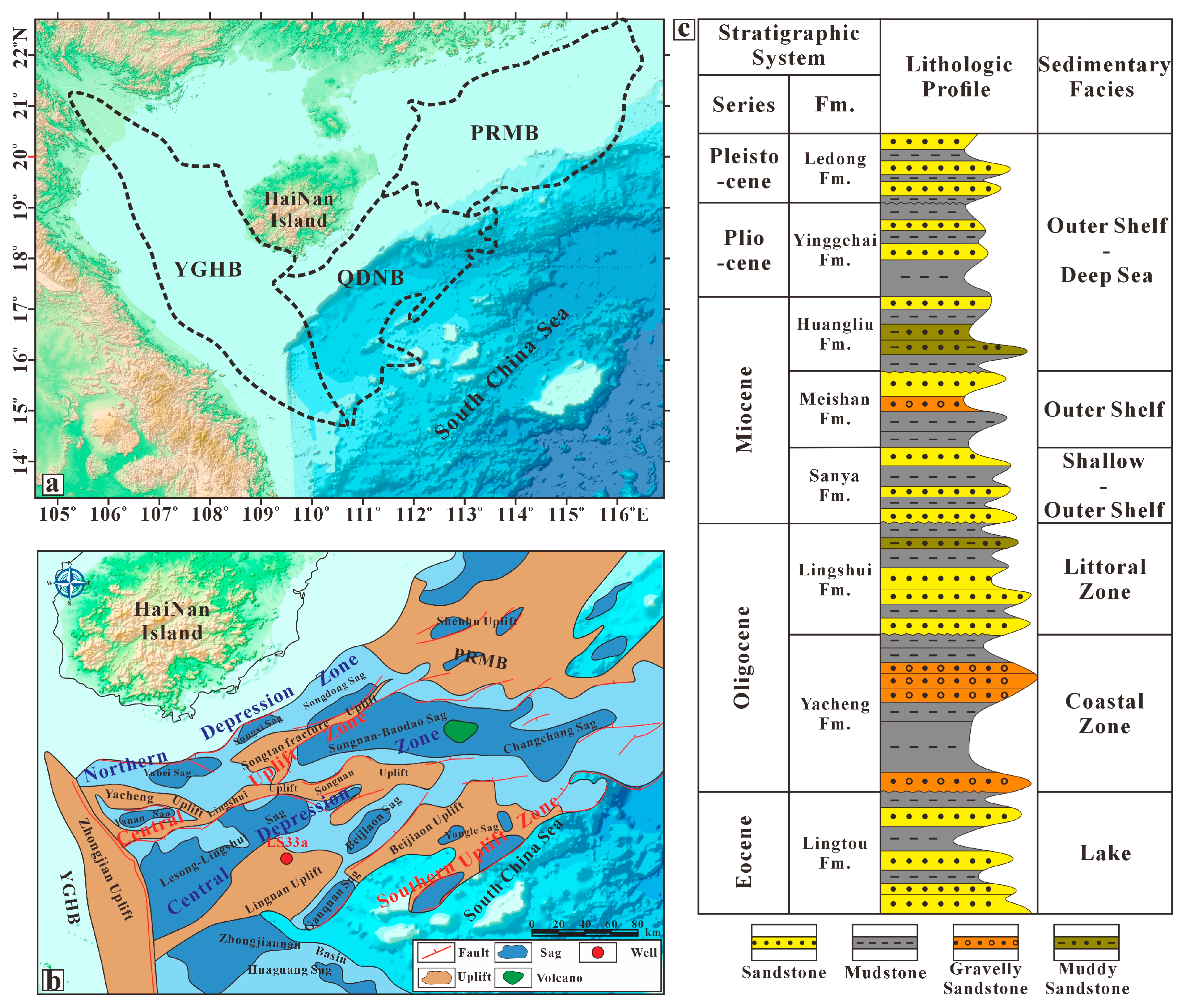
2. Regional Geological Setting

The Qiongdongnan Basin is situated along the western edge of the northern South China Sea, encompassing approximately 40,000 square kilometers. The basin’s development has been shaped by the complex interplay between the Pacific and Eurasian tectonic plates, alongside the seafloor spreading activities in the South China Sea. Geologically, it exhibits a northeastward trend. It is positioned geographically between Hainan Island and the Xisha (Paracel) Islands, with the Yinggehai Basin to its west and the Pearl River Mouth Basin’s Shenhu Uplift to the east (refer to Figure 1a,b). This basin is representative of extensional basins and has been formed over a geological timescale from the Paleocene through to the Quaternary period [29,30,31].
The basin trends predominantly in an east–west direction and has undergone two major evolutionary stages: the Paleogene rift stage and the Neogene subsidence stage. During the Paleogene rifting stage, fault development within the basin resulted in a characteristic “two depressions and one uplift” structural pattern. Based on structural features, the Qiongdongnan Basin is divided into four primary structural units: the Southern Uplift, the Central Depression Zone, the Central Uplift Zone, and the Northern Depression Zone. Additionally, multiple secondary structural units are developed within the basin, including the Changchang Depression, Songnan Depression, Baodao Depression, Lingshui Depression, Ledong Depression, Beijiao Depression, Yacheng Uplift, Songnan Low Uplift, and Songtao Uplift [10,32,33].
Based on structural, geophysical logging, seismic, and lithological data, the stratigraphy of the Qiongdongnan Basin is subdivided from bottom to top into the Lingtou Formation, Yacheng Formation, Lingshui Formation, Sanya Formation, Meishan Formation, Huangliu Formation, Yinggehai Formation, and Ledong Formation [6,32] (Figure 1c). The Upper Oligocene Lingshui Formation is further divided into three members, characterized by a north-thickening and south-thinning pattern, indicative of erosional processes during the late rifting stage. The lower part is dominated by transitional facies deposits, while the middle and upper parts consist of littoral clastics and semi-enclosed shallow marine sedimentary systems, with lithologies mainly comprising conglomerates, sandstones, and mudstones, along with localized unconformities [14,34]. In the LS33a borehole of the study area, the Lingshui Formation is predominantly composed of mudstones and silty mudstones, interbedded with thin layers of siltstone and argillaceous siltstone. These deposits reflect sedimentary characteristics of a littoral-to-shallow marine environment. Well LS33a is located within the Central Depression Zone of the Qiong Southeast region, and its unique geological background makes it an ideal object for the astronomical chronology and cyclostratigraphy research. During the Middle-Late Oligocene, the area was in a deep-water environment with relatively stable sedimentary conditions. The stable conditions during this period created an ideal environment for examining the astronomical forcing characteristics and cyclicity of the strata, thereby enhancing our understanding of the connections between sedimentary processes and climate change.

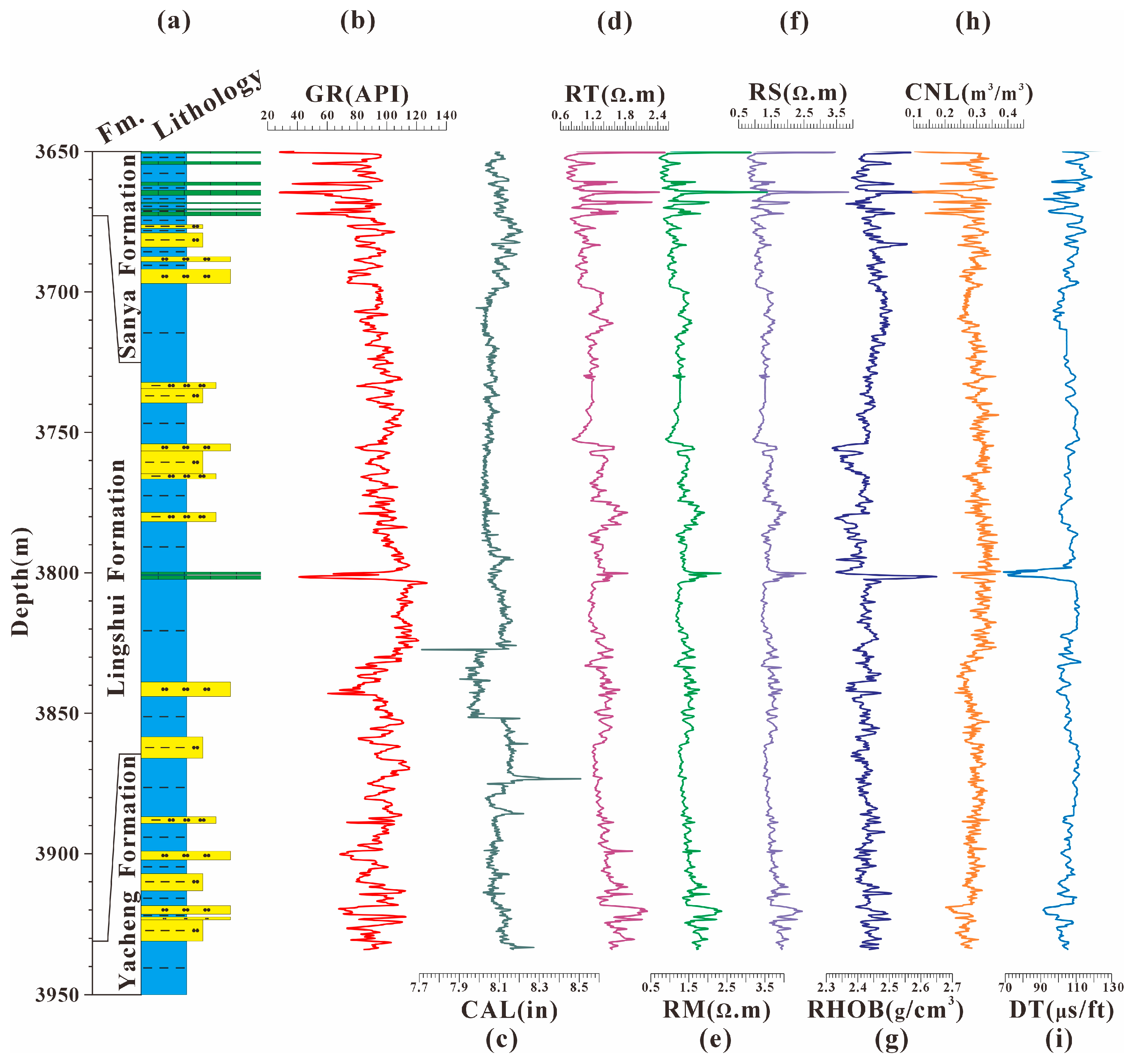
3. Materials and Methods

This study integrates planktonic foraminiferal data from the LS33a borehole and applies the modified Cenozoic planktonic foraminiferal zonation by Wade (2010) [35] to biostratigraphic zones in the Lingshui Formation. According to the International Chronostratigraphic Chart (v2023/09) [36], a chronological framework for the Lingshui Formation is established, which serves as a constraint for subsequent time series analysis. The Power Ratio Accumulation (PRA) method, combined with power decomposition, the null hypothesis of no astronomical forcing, and Monte Carlo simulations, effectively identifies the most astronomically sensitive proxy indicators from multiple sets of geophysical logging data [27]. This approach not only optimizes the selection of proxy indicators but also minimizes bias risks arising from incorrect proxy selection [28]. In this study, the PRA method was applied to analyze multiple geophysical logging datasets from the Lingshui Formation in the LS33a borehole. The most optimal paleoclimate proxy was ultimately selected for subsequent time series analysis.
Building on the optimal paleoclimate proxy selected via the PRA method, time series analysis includes the following steps:
Firstly, the data series undergo preprocessing (e.g., detrending, interpolation, and pre-whitening) to eliminate low-frequency signals that could affect the astronomical cycle analysis. Subsequently, the spectral analysis was performed, using the 2π Multi-taper Method (2πMTM), with the Robust AR(1) red noise model applied to test spectral significance [37,38]. Evolutionary spectral analysis is conducted using the Evolutionary Fast Fourier Transform (eFFT) to examine frequency variations and their stability within the depth domain [39]. Combining this approach with the astronomical cycle ratio method, the approximate cycle thickness was determined, and the average sedimentation rate is estimated. These results are then validated against the outcomes of the biostratigraphic framework.
In the analysis of sedimentation rates, the optimal sedimentation rate derived from the PRA method was triangulated with the results obtained from the correlation coefficient method (COCO/eCOCO) and the astronomical cycle ratio method to construct a more robust sedimentation rate framework [40]. Given the long-term stability of the 405 kyr long eccentricity cycle [41], Gaussian and Taner–Hilbert filters [39] were applied to extract the cycle thickness corresponding to the 405 kyr long eccentricity. This enabled the construction of an age model and subsequent tuning, converting the depth-domain data series into a time–domain data series. After obtaining the time–domain data series, we compared them in the frequency domain with the La2010d theoretical astronomical solution [41] to verify the reliability of their depth domain analysis results. Subsequently, we applied the 405 kyr long eccentricity filtering method from the La2010d theoretical astronomical solution and conducted astronomical tuning within the chronological framework established by the planktonic foraminifera zones, thereby constructing the astronomical timescale framework for the Lingshui Formation.
Additionally, sedimentary noise models (DYNOT and ρ1) were employed to model relative sea-level changes. The DYNOT model, based on noise source analysis of climate and sea-level proxy indicators, estimates sea-level variations by calculating the ratio of non-orbital signal variance to total signal variance. In contrast, the ρ1 model quantifies trend components in sea-level changes by analyzing the lag-1 autocorrelation coefficient of the time series [42].

4. Results

4.1. Chronological Framework Determined by Planktonic Foraminifera

In well LS33a (depth range 3650 m–3950 m), 12 major species of planktonic foraminifera were identified (Figure 2b). Among these, Chiloguembelina cubensis, Paragloborotalia opima, Paragloborotalia kugleri, and Globoquadrina dehiscens were identified as key zonal fossils (marked in red in Figure 2b).
In the LS33a borehole, the highest occurrence of Chiloguembelina cubensis is identified at 3934 m, marking its last occurrence (LO), which defines the upper boundary of the O4 zone (Figure 2) with a corresponding age of approximately 28.4 Ma [35,43]. Notably, the lower boundary of the Lingshui Formation is located at 3931 m, corresponding to the T70 seismic interface, which is also estimated to have an age of approximately 28.4 Ma [12]. Thus, the age of the lower boundary of the Lingshui Formation can be confidently assigned to 28.4 Ma, placing it within the Rupelian stage of the Oligocene [36].
The last occurrence (LO) of Paragloborotalia opima marks the upper boundary of the O5 zone, with an estimated age of approximately 27.75 Ma [35,43]. In the LS33a borehole, the highest occurrence of this species is identified at 3844 m (Figure 2). Internationally, the LO of Paragloborotalia pseudokugleri is typically used to define the upper boundary of the O6 zone [35]. However, this fossil was not observed in the LS33a borehole. The first occurrence (FO) of Paragloborotalia kugleri is recognized as the upper boundary of the O7 zone [35], with the lowest occurrence of this species also recorded at 3844 m in the LS33a borehole. Nevertheless, due to the potential risk of sample loss in cuttings, the minimum depth of occurrence at 3844 m may not be entirely accurate.
The first occurrence (FO) of Globoquadrina dehiscens marks the lower boundary of the M1b zone, with an estimated age of approximately 23.2 Ma [35,43]. In the LS33a borehole, the lowest occurrence of this fossil is identified at 3691 m (Figure 2). Additionally, the upper boundary of the Lingshui Formation is located at 3762 m, corresponding to the T60 seismic interface, with an estimated age of 23.03 Ma [12,14]. This age aligns well with the FO of Globoquadrina dehiscens, providing mutual corroboration. However, due to the uncertainties associated with its FO, this age is subject to some degree of uncertainty.
In summary, based on biostratigraphic analysis, the Lingshui Formation in the LS33a borehole includes the planktonic foraminiferal O5 zone, the combined O6-O7-M1a zone, and the lower part of the M1b zone. Its age spans approximately 28.4 Ma to 23.03 Ma, suggesting that its formation occurred during the early Chattian stage of the late Oligocene, although deposition may have begun in the late Rupelian stage.

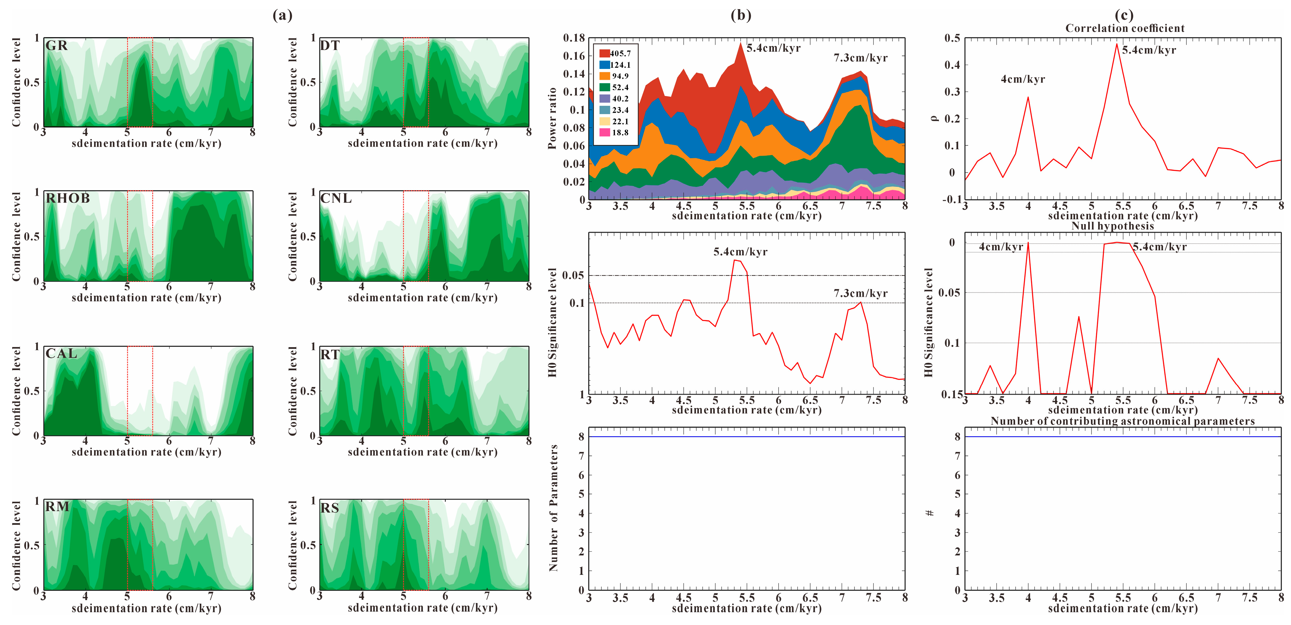
4.2. Optimal Paleoclimate Proxy

Through planktonic foraminiferal zonation analysis, the chronological framework for the 3950–3650 m depth interval in the LS33a borehole was established, with an estimated average sedimentation rate of approximately 5.3 cm/kyr. A Power Ratio Accumulation (PRA) sensitivity analysis was performed on all geophysical logging data for this interval (Figure 3). The obtained results (Figure 4a) indicate that the natural gamma ray (GR) data exhibited extremely high astronomical forcing sensitivity within the sedimentation rate range of 5–5.6 cm/kyr. The gamma ray data have shown a closer correlation with the astronomical forcing with respect to the geophysical logs.
Subsequently, further PRA analysis was conducted on the GR data (Figure 4b), revealing two significant values corresponding to sedimentation rates of 5.4 cm/kyr and 7.3 cm/kyr. However, the H₀ significance level at 7.3 cm/kyr was below 0.1%, while at 5.4 cm/kyr, it was below 0.05%. Based on the PRA analysis, the optimal sedimentation rate was estimated to be 5.4 cm/kyr.
Additionally, the correlation coefficient method (COCO) analysis was performed on the GR data (Figure 4c), which also identified two significant values, corresponding to sedimentation rates of 4.0 cm/kyr and 5.4 cm/kyr. Combining the chronological framework provided by biostratigraphy with the results of PRA and COCO analyses, the optimal sedimentation rate range for the deposition of the Lingshui Formation is inferred to be 5–5.4 cm/kyr.

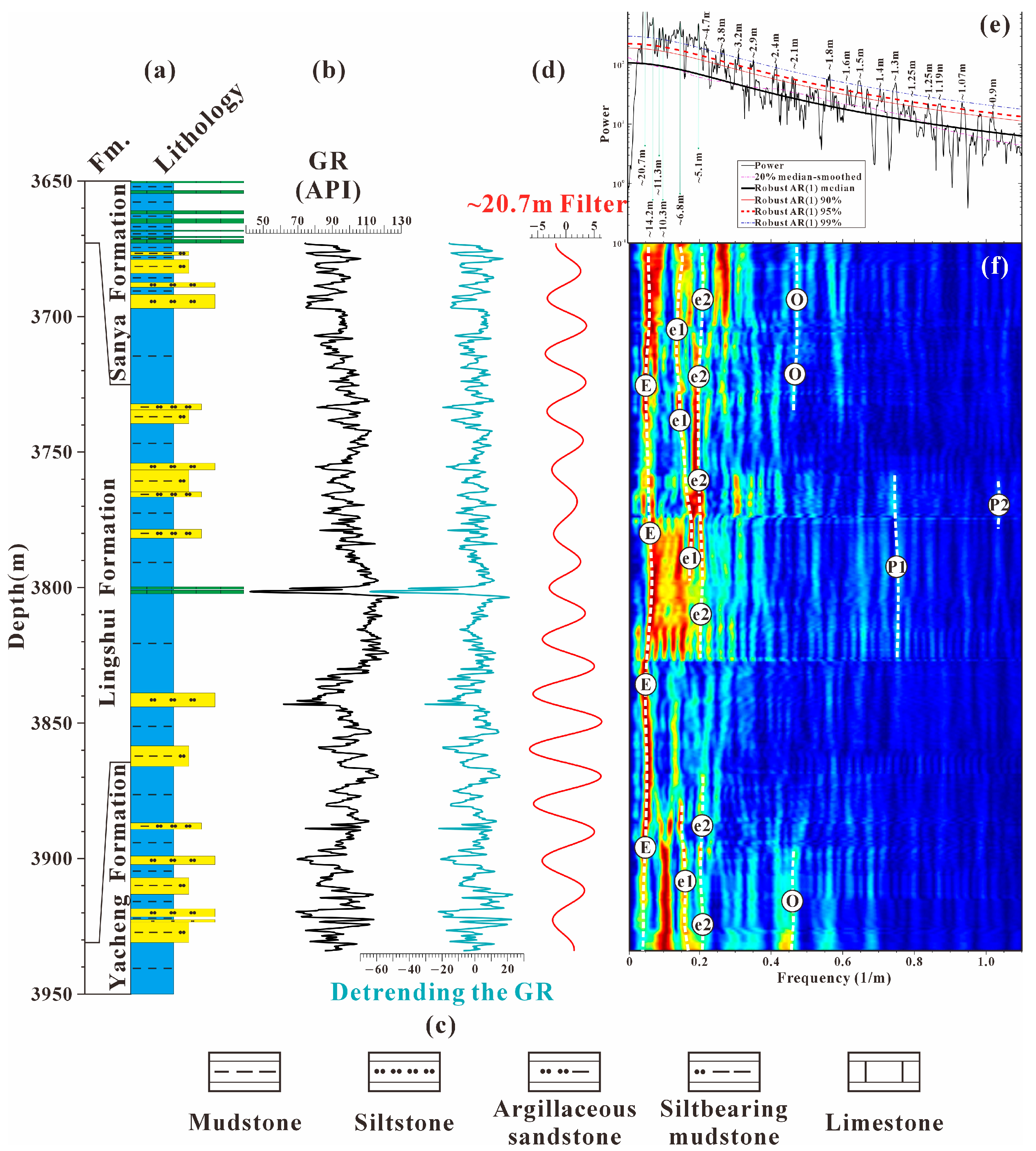
4.3. Time Series Analysis

The 2πMTM spectral analysis of the GR data series has revealed several significant dominant peaks (Figure 5e). Further evolutionary spectral analysis using eFFT indicated that a cycle thickness of ~20.7 m exhibits high stability (Figure 5f), which may correspond to the 405 kyr long eccentricity cycle due to its well-established stability over long timescales [23,41].
According to the La2010d theoretical astronomical solution for the late Oligocene to early Miocene [41], the eccentricity cycles include 405.7 kyr, 124.1 kyr, and 94.9 kyr; obliquity cycles include 52.4 kyr and 40.2 kyr; and precession cycles include 23.4 kyr, 22.1 kyr, and 18.8 kyr. The analysis revealed that cycle thicknesses of ~20.7 m, ~6.8 m, ~4.7 m, ~2.1 m, ~1.19 m, and ~0.9 m exhibit ratios that closely match the period ratios of eccentricity and obliquity and precession in the La2010d solution. This strongly suggests that significant astronomical signals are preserved in the GR data series.
Further analysis inferred that if the ~20.7 m cycle thickness corresponds to the 405.7 kyr long eccentricity cycle, the optimal average sedimentation rate for the 3934–3673 m interval of the LS33a borehole is approximately 5.1 cm/kyr. This result aligns closely with the sedimentation rate range of 5–5.4 cm/kyr derived from PRA and COCO analyses, thereby validating the assumptions proposed by the astronomical cycle ratio method as reasonable and reliable.
Filtering the ~20.7 m cycle thickness (Figure 5d) allowed for the 405 kyr astronomical cycle adjustment of the data series, constructing an age model. Subsequently, the depth-domain data series was converted into a time–domain data series using tuning methods (Figure 6b).
In the 405 kyr tuned GR time series, 2πMTM spectral analysis clearly identified various orbital parameters (Figure 6a), which exhibit a high degree of consistency with the periods predicted by the La2010d theoretical astronomical solution. Additionally, the wavelet power spectrum of the 405 kyr tuned GR time series (Figure 6c) displays strong astronomical forcing characteristics, further validating the reliability of the astronomical signals in the sequence.
Based on this analysis, the floating astronomical age of the 3934–3673 m strata in the LS33a borehole (covering the top of the Yacheng Formation and the Lingshui Formation) is approximately 5078.099 kyr (Figure 6b,c).

4.4. Astronomical Chronology Analysis

Based on the results of planktonic foraminiferal zonation, the chronological framework for the Lingshui Formation in the LS33a borehole is approximately between the late Rupelian and late Chattian stages. For the 3934–3673 m strata (covering the top of the Yacheng Formation and the Lingshui Formation), the floating astronomical age is estimated to be approximately 5078.099 kyr.
The age at a depth of ~3934 m in the LS33a borehole is roughly constrained to 28.4 Ma based on the last occurrence (LO) of Chiloguembelina cubensis. The 405 kyr filtering reveals that this section contains approximately 12.5 cycles of the 405 kyr long eccentricity cycle. Comparison and tuning of this sequence with the 405 kyr filtering results of the La2010d theoretical astronomical orbital solution (21–29 Ma) (Figure 7f) show that its cyclic characteristics correspond closely to the E71 to E59 stages of the theoretical eccentricity cycle (Figure 7).
According to the tuning results, the base of the Lingshui Formation (3931 m) corresponds to the E71 eccentricity cycle, while the top (3672.85 m) corresponds to half a cycle of E59. The absolute astronomical age range for the Lingshui Formation is thus calculated to be 28.52 Ma to 23.5 Ma, with a duration of 5.02 Ma. Yang et al. (2024) conducted a cyclostratigraphic analysis of the Lingshui Formation and proposed that the basal interface of the formation corresponds to 28.51 Ma [14]. This result is nearly consistent with our findings, thereby validating the accuracy of the astronomical tuning.

4.5. Sedimentary Noise Modeling and Astronomical Forcing

Sedimentary noise modeling was performed on the 405 kyr tuned GR time series using the DYNOT and ρ1 models (Figure 8e,g). The DYNOT and ρ1 models have been demonstrated to be objective and accurate tools for reconstructing paleosea-level or paleolake-level changes [42,44,45,46,47]. The analysis results indicate that the sea-level in the Lingshui Formation region of the LS33a borehole experienced approximately five prominent cycles of rise and fall during the deposition period.
Further spectral analysis of the DYNOT and ρ1 models (Figure 8h,i) revealed a significant dominant spectral peak at the 1.2 Myr cycle. The 1.2 Myr cycle, recognized as the Earth’s obliquity modulation cycle (s4-s3 term), is known to have a critical influence on global and regional climate and sea-level fluctuations [48,49,50].
Gaussian bandpass filtering (passband: 0.00247 ± 0.00043 cycles/kyr) was applied to the median time series of the DYNOT and ρ1 models to extract the 1.2 Myr periodic variation characteristics. The results indicate that approximately five 1.2 Myr cycles occurred during the deposition period of the Lingshui Formation.
Comparison of this cycle with sea-level rise and fall variations (Figure 8d–g) reveals that sea-level changes were strongly controlled by the ~1.2 Myr cycle. This pattern highlights the significant astronomical forcing of sea-level changes during the deposition period of the Lingshui Formation and further supports the presence of astronomical cycles in the stratigraphic record.

5. Discussion

5.1. Geophysical Logging as a Proxy

Paleoclimate proxies are crucial tools for studying past climate changes and are generally categorized into two main types. The first type involves direct measurements from borehole cores and field outcrops, such as magnetic susceptibility, stable isotopes, rock color, lithology, and biological indicators [27,28,51,52,53,54,55]. Although these proxies are widely used in cyclostratigraphic and astrochronological studies, their application is limited by several factors. On one hand, obtaining complete core samples is challenging, and the number of available field outcrops is relatively limited. On the other hand, the process of acquiring these indicators often involves substantial technical and labor costs [28]. These factors constrain their application in large-scale studies.
Another category of proxies is geophysical logging data, which includes measurements like natural gamma radiation, resistivity, sonic interval transit time, and density. These data are acquired directly from the in-situ strata using geophysical logging instruments within boreholes, providing insights into the physical and chemical properties of the strata [27,28,56,57,58]. Compared to direct measurement proxies, geophysical logging data offer advantages such as high resolution, continuous sampling, diverse parameters, objective accuracy, and cost effectiveness [27,58,59,60].
In this study, a Power Ratio Accumulation (PRA) method was used to perform sensitivity analysis on eight types of geophysical logging data from the Lingshui Formation section in well LS33a (Figure 3 and Figure 4a). The results indicate that among the eight data types, natural gamma (GR) is the most sensitive to astronomical forcing, and the optimal sedimentation rate it reflects is highly consistent with previous analyses. GR measures the intensity of gamma rays emitted during the decay of naturally occurring radionuclides in the strata [61]. In sedimentary layers, gamma ray intensity exhibits a positive correlation with mudstone content. This relationship primarily arises from the fact that fine-grained mudstone has a larger specific surface area, enhancing its capacity to adsorb radioactive substances [28]. Furthermore, gamma ray (GR) measurements are widely utilized in cyclostratigraphy studies of marine strata [10,14,25,27,62,63,64]. This widespread application reflects the high sensitivity of GR and its broad applicability to astronomical forcing.
Despite the advantages of gamma ray (GR) measurements in cyclostratigraphy, their widespread application raises potential concerns. Many studies fail to critically assess the use of GR, which can result in inaccuracies in certain contexts. While GR may serve as a suitable paleoclimate proxy in some regions, its reliability can vary significantly elsewhere. To address these issues, this study employs the Power Ratio Accumulation (PRA) method to identify optimal paleoclimate proxies from diverse geophysical logging data. This approach not only enhances the reliability of the analysis but also provides valuable insights into astronomical forcing within complex sedimentary systems.
It is also important to note that geophysical logging data, as secondary paleoclimate proxies [19], primarily reflect some indirect properties related to astronomical forcing, such as clay mineral content. The relationship between these properties and paleoclimate change is more complex. Therefore, in cyclostratigraphy research, a comprehensive validation approach using multiple parameters and techniques should be employed to enhance the robustness of experimental results and avoid biases introduced by relying on a single proxy.

5.2. Sea-Level Change Under Astronomical Forcing

The rise and fall of global sea-levels are closely related to astronomical forcing [65,66,67,68]. When the Earth’s orbital tilt increases, the solar radiation received by the Northern Hemisphere also increases, leading to enhanced melting of land glaciers and a subsequent rise in sea-level. Conversely, when the orbital tilt decreases, solar radiation in the Northern Hemisphere diminishes, allowing land glaciers to be preserved, which causes sea-level to fall (Figure 9j,k) [69,70].
In this study, we utilized a 405 kyr tuned GR time series to reconstruct ancient sea-level changes during the Lingshui Formation sedimentation period using the DYNOT and ρ1 sediment noise models (see Figure 8e,g). We conducted a spectral analysis of the medians from both DYNOT and ρ1 sediment noise models (Figure 8h,i) and identified a significant signal of approximately 1.2 Myr, which we interpret as the orbital tilt modulation period (s4-s3 term) that dominated sea-level fluctuations in the study area (see the blue and orange bands in Figure 8).
To compare the relationship between the study area and global sea-level changes as well as their astronomical theories, we adopted global sea-level data from 23 to 29 Ma [71] (Figure 9g) and the theoretical astronomical solution ETP from the La2010d model [41] for the same period (Figure 9i) as the reference. During the Lingshui Formation sedimentation period, approximately four significant cycles of sea-level rise and fall were observed (Figure 9c,e), which correspond to the same four notable rising and falling cycles in global sea-level during that period (Figure 9g). By applying Gaussian bandpass filtering to the global sea-level data from 23 to 29 Ma (with a passband of 0.00089 ± 0.00026 cycles/kyr, see Figure 9f), we found consistency between our results and the ETP’s Earth orbital tilt modulation period of ~1.2 Myr (Figure 9h). This aligns well with the 1.2 Myr periodic filtering results obtained through our DYNOT and ρ1 sediment noise models (Figure 9b,d). These findings support our conclusions in Section 4.5, providing strong evidence that global sea-level is controlled by the ~1.2 Myr orbital tilt modulation period. Furthermore, the good correspondence among global sea-level, theoretical astronomical solutions, and sediment noise models validates the accuracy of the astronomical timescale framework we established for the Lingshui Formation.
However, due to the complexity of the Earth’s system, sea-level changes are influenced by multiple factors [72]. Over long-time scales, the controlling influence of astronomical cycles on sea-levels is very evident; however, the extent to which these cycles dictate sea-level changes over shorter time scales requires further investigation. The modeling of the DYNOT sediment noise model can adjust the recovery resolution of sea-levels by changing the window size. Smaller windows increase the resolution but simultaneously reduce the low-frequency cycle variance and total variance, thus increasing the uncertainty in estimating non-orbital signal ratios. Therefore, questions regarding sea-level changes at shorter time scales are also limited by technical means.

6. Conclusions

This study has revealed, through PRA sensitivity analysis, the high sensitivity of natural gamma ray (GR) logging to astronomical forcing, making it an effective proxy for paleoclimatic research. Time series analysis demonstrated that the Lingshui Formation retains distinct astronomical periodic signals. By utilizing the COCO and PRA methods, we identified the optimal sedimentation rate of the Lingshui Formation in well LS33a to be 5–5.4 cm/kyr and constructed an astronomical timescale framework corresponding to the late Oligocene, from the late Rupelian to Chattian stages (28.52–23.5 Ma) through astronomical tuning. Additionally, by utilizing the DYNOT and ρ1 sediment noise models, we analyzed sea-level changes during the sedimentation period of the Lingshui Formation. This analysis identified a dominant 1.2 Myr periodicity influencing sea-level, which was then compared with global sea-level changes data and the La2010d theoretical astronomical solution. We found that the sea-level changes in the study area are consistent with global sea-level changes, both influenced by the 1.2 Myr orbital obliquity modulation period.
This research not only reconstructed the astronomical timescale framework for the Lingshui Formation in well LS33a but also explored the astronomical forcing effects on sea-level in depth. It provides a methodological framework for future studies: constraining stratigraphic frameworks, identifying optimal paleoclimate proxies, employing multiple methods such as PRA and COCO to validate depth domain analysis results, and implementing astronomical tuning to establish astronomical timescales for stratigraphy, thereby reducing the risk of Type I errors. However, there are some limitations in this study: the applicability of the stratigraphic framework methods at the regional scale may be constrained, and the complexity of local geological conditions has not been fully considered. Moreover, due to the resolution and quality of available data, the inferences regarding sea-level changes may not encompass all potential external factors. Therefore, future research should further explore sedimentation patterns in different environments and geological contexts and integrate more datasets to provide a more comprehensive model of sea-level changes.

Author Contributions

Conceptualization, S.Z. and Y.W.; methodology, J.L. and Y.W.; software, J.L. and G.G. and R.H.; validation, J.L. and Y.L.; formal analysis, S.Z.; investigation, Y.W. and S.Z.; resources, S.Z.; data curation, Y.W. and S.Z.; writing—original draft preparation, J.L.; writing—review and editing, J.L. and Y.W. and S.Z.; visualization, Y.L.; supervision, S.Z. and G.G.; project administration, Y.W. and S.Z.; funding acquisition, S.Z. and Y.W. All authors have read and agreed to the published version of the manuscript.

Funding

This research was funded by [The National Natural Science Foundation of China], grant number [41472098].

Institutional Review Board Statement

Not applicable.

Informed Consent Statement

Not applicable.

Data Availability Statement

All data and materials are sourced from the National Natural Science Foundation of China (Project No. 41472098) entitled “Sea-Level Changes and Sequence Stratigraphic Models of the Double Slope Belt on the Northern South China Sea Shelf.” Relevant data and materials can be obtained from the corresponding authors upon request. It is important to note that some data cannot be publicly disclosed as ongoing research is utilizing these datasets.

Acknowledgments

The authors are grateful to Enze Xu for his insightful methodological suggestions provided during the initial stages of this research. The author would like to express special thanks to the four anonymous reviewers for their valuable suggestions, which enabled the completion of this article.

Conflicts of Interest

The authors declare no conflicts of interest.

References

  1. Xue, L.; Ding, X.; Pei, R.; Wan, X. Miocene paleoenvironmental evolution based on benthic foraminiferal assemblages in the Lufeng Sag, Northern South China Sea. Acta Oceanol. Sin. 2019, 38, 124–137. [Google Scholar] [CrossRef]
  2. Zhao, S.; Wang, Y.; Zhang, S.; Zhu, R.; Xu, E.; YI, Z.; Gong, G.; Wang, Y.; Liu, H. Miocene Paleoclimate Analysis of the Northern South China Sea: Response to Cooling Events Based on Astronomical Cycles. Mar. Geol. Front. 2022, 38, 53–62. (In Chinese) [Google Scholar] [CrossRef]
  3. Zhao, Q.; Wang, P. Progress in Quaternary Paleoceanography of the South China Sea: A Review. Quat. Sci. 1999, 19, 481–501. (In Chinese) [Google Scholar]
  4. Liu, X.; Xie, J.; Zhang, H.; He, W. Chronostratigraphy of Planktonic Foraminifera in the Yinggehai-Qiongdongnan Basin. Acta Micropalaeontol. Sin. 2009, 26, 181–192. (In Chinese) [Google Scholar]
  5. Cheng, S.; Li, S.; Suo, Y.; Liu, X.; Yu, S.; Dai, L.; Ma, Y.; Zhao, S.; Wang, X.; An, H.; et al. Cenozoic Tectonics and Dynamics of Basin Groups of the Northern South China Sea. Mar. Geol. Quat. Geol. 2012, 32, 79–93. (In Chinese) [Google Scholar] [CrossRef]
  6. Liu, S.; Chen, H.; Li, D.; Shun, W.; Li, C. Sedimentary characteristics and source rock development model of the Oligocene Lingshui Formation in Lingshui Sag, Qiongdongnan Basin. Mar. Orig. Pet. Geol. 2019, 24, 63–70. (In Chinese) [Google Scholar]
  7. Xie, H.; Zhou, D.; Shi, H.; Li, Y.; Kong, D. Comparative study on the Cenozoic tectonic and sedimentary evolution in the deep water areas of the Zhujiang River Estuary Basin and the Qiongdongnan Basin. Haiyang Xuebao 2021, 43, 48–61. (In Chinese) [Google Scholar]
  8. Zhu, J.; Yang, X.; Hu, X.; Luo, W.; Li, Y.; Mao, X.; Feng, S. Characteristic and petroleum geology of the Mesozoic sags of the northern Qiongdongnan Basin. Bull. Geol. Sci. Technol. 2023, 42, 83–93. (In Chinese) [Google Scholar] [CrossRef]
  9. Xu, C.; You, L. North slope transition zone of Songnan–Baodao sag in Qiongdongnan Basin and its control on medium and large gas fields, South China Sea. Pet. Explor. Dev. 2022, 49, 1061–1072. (In Chinese) [Google Scholar] [CrossRef]
  10. Zhang, S.; Xu, M.; Tang, W.; Xu, E.; Wang, Y.; Zhu, R. Cyclostratigraphy and paleoclimate analysis of Lingshui Formation in Beijiao Sag, Qiongdongnan Basin. Bull. Geol. Sci. Technol. 2024, 1–13. (In Chinese) [Google Scholar] [CrossRef]
  11. Wu, K.; Xie, X.; Pei, J.; Ren, J.; You, L.; Jiang, T.; Quan, Y. Deep architecture of hyperextended marginal basin and implications for hydrocarbon exploration: A case study of Qiongdongnan Basin. Oil Gas Geol. 2023, 44, 651–661. (In Chinese) [Google Scholar]
  12. Ding, W.; Hou, D.; Gan, J.; Wu, P.; Zhang, M.; George, S.C. Palaeovegetation variation in response to the late Oligocene-early Miocene East Asian summer monsoon in the Ying-Qiong Basin, South China Sea. Palaeogeogr. Palaeoclimatol. Palaeoecol. 2021, 567, 110205. [Google Scholar] [CrossRef]
  13. Cao, H.; Jin, S.; Hou, M.; Chen, S.; Liu, Y.; Chen, A. Astronomical cycles calibrated the sea-level sequence durations of Late Miocene to Pliocene in Qiongdongnan Basin, south China sea. Mar. Pet. Geol. 2022, 143, 105813. [Google Scholar] [CrossRef]
  14. Yang, H.; Tang, W.; Xu, E.; Zhang, S.; Wang, Y.; Xu, M. Cyclostratigraphy and paleoclimate analysis of the Lingshui Formation in Changchang Sag, Qiongdongnan Basin, China. Energy Geosci. 2024, 5, 100224. [Google Scholar] [CrossRef]
  15. Liu, X.; Sun, Z.; Liu, X.; Liu, D.; Zhai, S.; Long, H.; Jiang, L.; Bi, D. Chronostratigraphic Framework based on Micro-paleontological Data from Drilling LS33a in Deep Water Area of Northern South China Sea. Acta Sedimentol. Sin. 2018, 36, 890–902. (In Chinese) [Google Scholar] [CrossRef]
  16. Zhao, M. Evolution of Paleoenvironment in the Qiongdongnan Basin During the Cenozoic. Master’s Thesis, Ocean University of China, Qingdao, China, 2013. [Google Scholar]
  17. Hilgen, F.J.; Hinnov, L.A.; Abdul Aziz, H.; Abels, H.A.; Batenburg, S.; Bosmans, J.H.; de Boer, B.; Hüsing, S.K.; Kuiper, K.F.; Lourens, L.J. Stratigraphic Continuity and Fragmentary Sedimentation: The Success of Cyclostratigraphy as Part of Integrated Stratigraphy; The Geological Society of London: London, UK, 2015. [Google Scholar]
  18. Sageman, B.B.; Singer, B.S.; Meyers, S.R.; Siewert, S.E.; Walaszczyk, I.; Condon, D.J.; Jicha, B.R.; Obradovich, J.D.; Sawyer, D.A. Integrating 40Ar/39Ar, U-Pb, and astronomical clocks in the Cretaceous Niobrara Formation, Western Interior Basin, USA. Bulletin 2014, 126, 956–973. [Google Scholar] [CrossRef]
  19. Meyers, S.R. Cyclostratigraphy and the problem of astrochronologic testing. Earth-Sci. Rev. 2019, 190, 190–223. [Google Scholar] [CrossRef]
  20. Fang, Y.; Olsen, P.; Zheng, D.; Xue, N.; Wang, H.; Xu, C.; Li, S.; Wang, B.; Zhang, H. A new astronomical time scale for the early Jehol Biota in the Luanping Basin, northeastern China. Palaeogeogr. Palaeoclimatol. Palaeoecol. 2022, 607, 111273. [Google Scholar] [CrossRef]
  21. Olsen, P.E.; Kent, D.V. Milankovitch climate forcing in the tropics of Pangaea during the Late Triassic. Palaeogeogr. Palaeoclimatol. Palaeoecol. 1996, 122, 1–26. [Google Scholar] [CrossRef]
  22. Wu, H.; Zhang, S.; Hinnov, L.A.; Jiang, G.; Feng, Q.; Li, H.; Yang, T. Time-calibrated Milankovitch cycles for the late Permian. Nat. Commun. 2013, 4, 2452. [Google Scholar] [CrossRef] [PubMed]
  23. Hinnov, L.A. Cyclostratigraphy and astrochronology in 2018. In Stratigraphy & Timescales; Elsevier: Amsterdam, The Netherlands, 2018; Volume 3, pp. 1–80. [Google Scholar]
  24. Huang, C. Astronomical time scale for the Mesozoic. In Stratigraphy & Timescales; Elsevier: Amsterdam, The Netherlands, 2018; Volume 3, pp. 81–150. [Google Scholar]
  25. Wei, X.; Yan, D.; Wang, D.; Fu, H. Astronomically forced paleoclimate and sea-level changes recorded in the continental margin of the South China Sea over the past ~23 m.y. GSA Bull. 2024, 136, 3553–3568. [Google Scholar] [CrossRef]
  26. Huang, C.; Ogg, J.G.; Kemp, D.B. Cyclostratigraphy and astrochronology: Case studies from China. Palaeogeogr. Palaeoclimatol. Palaeoecol. 2020, 560, 110017. [Google Scholar] [CrossRef] [PubMed]
  27. Peng, C.; Zou, C.; Wu, H.; Zhang, S.; Kouamelan, K.S.; Wang, C. Evaluating geophysical logs as proxies for cyclostratigraphy in lacustrine deposits using power ratio accumulation. Palaeogeogr. Palaeoclimatol. Palaeoecol. 2023, 614, 111428. [Google Scholar] [CrossRef]
  28. Peng, C.; Zou, C.; Zhang, S.; Shu, J.; Wang, C. Geophysical logs as proxies for cyclostratigraphy: Sensitivity evaluation, proxy selection, and paleoclimatic interpretation. Earth-Sci. Rev. 2024, 252, 104735. [Google Scholar] [CrossRef]
  29. Xie, W.; Zhang, Y.; Sun, Z.; Jiang, J. Characteristics and Formation Mechanism of Faults in the Qiongdongnan Basin. Mar. Geol. Quat. Geol. 2007, 27, 71–78. (In Chinese) [Google Scholar] [CrossRef]
  30. Qiu, N.; Wang, Z.; Wang, Z.; Sun, Z.; Sun, Z.; Zhou, D. Tectonostratigraphic Structure and Crustal Extension of the Qiongdongnan Basin, Northern South China Sea. Chin. J. Geophys. 2014, 57, 3189–3207. (In Chinese) [Google Scholar]
  31. Li, C.; You, L.; Zhu, J.; Yang, J.; Wang, L. Effect of Fault Systems on Hydrocarbon Accumulation in the Central Depression Below the Deep Sea, Qiongdongnan Basin. Mar. Orig. Pet. Geol. 2016, 21, 73–78. (In Chinese) [Google Scholar]
  32. Shao, L.; Li, A.; Wu, G.; Li, Q.; Liu, C.; Qiao, P. Evolution of Sedimentary Environment and Provenance in the Qiongdongnan Basin, Northern South China Sea. Acta Pet. Sin. 2010, 31, 548–552. (In Chinese) [Google Scholar]
  33. Li, Y.; Deng, Y.; Zhang, G. Zoned Distribution of Source Rocks and Hydrocarbons Offshore China. China Offshore Oil Gas 2012, 24, 6–12. (In Chinese) [Google Scholar]
  34. Wang, Z.; Li, X.; Sun, Z.; Huang, B.; Zhu, J.; Yao, Z.; Guo, M. Hydrocarbon Accumulation Conditions and Exploration Potential in the Deep-Water Region, Qiongdongnan Basin. China Offshore Oil Gas 2011, 23, 7–13+31. (In Chinese) [Google Scholar]
  35. Wade, B.S.; Pearson, P.N.; Berggren, W.A.; Pälike, H. Review and revision of Cenozoic tropical planktonic foraminiferal biostratigraphy and calibration to the geomagnetic polarity and astronomical time scale. Earth-Sci. Rev. 2011, 104, 111–142. [Google Scholar] [CrossRef]
  36. Cohen, K.M.; Finney, S.C.; Gibbard, P.L.; Fan, J.X. The ICS International Chronostratigraphic Chart. Int. Union Geol. Sci. 2013, 36, 199–204. [Google Scholar] [CrossRef] [PubMed]
  37. Thomson, D.J. Spectrum estimation and harmonic analysis. Proc. IEEE 1982, 70, 1055–1096. [Google Scholar] [CrossRef]
  38. Mann, M.E.; Lees, J.M. Robust estimation of background noise and signal detection in climatic time series. Clim. Chang. 1996, 33, 409–445. [Google Scholar] [CrossRef]
  39. Kodama, K.P.; Hinnov, L.A. Rock Magnetic Cyclostratigraphy; John Wiley & Sons: Hoboken, NJ, USA, 2014; Volume 5. [Google Scholar]
  40. Li, M.; Kump, L.R.; Hinnov, L.A.; Mann, M.E. Tracking variable sedimentation rates and astronomical forcing in Phanerozoic paleoclimate proxy series with evolutionary correlation coefficients and hypothesis testing. Earth Planet. Sci. Lett. 2018, 501, 165–179. [Google Scholar] [CrossRef]
  41. Laskar, J.; Fienga, A.; Gastineau, M.; Manche, H. La2010: A new orbital solution for the long-term motion of the Earth. Astron. Astrophys. 2011, 532, A89. [Google Scholar] [CrossRef]
  42. Li, M.; Hinnov, L.A.; Huang, C.; Ogg, J.G. Sedimentary noise and sea levels linked to land–ocean water exchange and obliquity forcing. Nat. Commun. 2018, 9, 1004. [Google Scholar] [CrossRef] [PubMed]
  43. Berggren, W.A.; Kent, D.V.; Swisher, C.C., III; Aubry, M.-P. A Revised Cenozoic Geochronology and Chronostratigraphy. Geochronol. Time Scales Glob. Stratigr. Correl. 1995, 54, 129–212. [Google Scholar] [CrossRef]
  44. Tang, Y.; Zheng, M.; Wang, X.; Wang, T.; Cheng, H.; Hei, C. The floating astronomical time scale for the terrestrial Early Permian Fengcheng Formation from the Junggar Basin and its stratigraphic and palaeoclimate implications. Geol. J. 2022, 57, 4842–4856. [Google Scholar] [CrossRef]
  45. Li, Y.; Yang, R.; Fan, A.; Chen, J.; Bilal, A.; Wang, Z. Establishment of a high-resolution astronomical time scale and high-frequency sequence framework of Paleogene lacustrine fine-grained sediments using logging data: A case study from the Bohai Bay Basin, East China. Mar. Pet. Geol. 2025, 172, 107220. [Google Scholar] [CrossRef]
  46. Liu, S.; Jin, S.; Liu, Y.; Chen, A. Astronomical forced sequence infill of Early Cambrian Qiongzhusi organic-rich shale of Sichuan Basin, South China. Sediment. Geology 2022, 440, 106261. [Google Scholar] [CrossRef]
  47. Falahatkhah, O.; Serajamani, M.; Kadkhodaie, A.; Aïfa, T.; Ebrahimi, S.; Ciabeghodsi, A.A.; Zamanzadeh, S.M.; Sfidari, E.; Vahidinia, M.; Ghaderi, A. Orbital obliquity evolution during the late Paleozoic ice age across the northeastern gondwana: Implications for regional sea-level change trigger and reservoir quality assessment. Mar. Pet. Geol. 2023, 153, 106312. [Google Scholar] [CrossRef]
  48. Falahatkhah, O.; Kordi, M.; Fatemi, V.; Koochi, H.H. Recognition of Milankovitch cycles during the Oligocene–Early Miocene in the Zagros Basin, SW Iran: Implications for paleoclimate and sequence stratigraphy. Sediment. Geol. 2021, 421, 105957. [Google Scholar] [CrossRef]
  49. Liu, Y.; Huang, C.; Ogg, J.G.; Algeo, T.J.; Kemp, D.B.; Shen, W. Oscillations of global sea-level elevation during the Paleogene correspond to 1.2-Myr amplitude modulation of orbital obliquity cycles. Earth Planet. Sci. Lett. 2019, 522, 65–78. [Google Scholar] [CrossRef]
  50. Zou, Z.; Huang, C.; Li, M.; Zhang, Y. Climate change response to astronomical forcing during the Oligocene-Miocene transition in the equatorial Atlantic (ODP Site 926). Sci. China Earth Sci. 2016, 59, 1665–1673. [Google Scholar] [CrossRef]
  51. Shi, J.; Jin, Z.; Liu, Q.; Zhang, R.; Huang, Z. Cyclostratigraphy and astronomical tuning of the middle eocene terrestrial successions in the Bohai Bay Basin, Eastern China. Glob. Planet. Chang. 2019, 174, 115–126. [Google Scholar] [CrossRef]
  52. Tian, J.; Xie, X.; Ma, W.; Jin, H.; Wang, P. X-ray fluorescence core scanning records of chemical weathering and monsoon evolution over the past 5 Myr in the southern South China Sea. Paleoceanography 2011, 26, 1r17. [Google Scholar] [CrossRef]
  53. Weedon, G.P.; Page, K.N.; Jenkyns, H.C. Cyclostratigraphy, stratigraphic gaps and the duration of the Hettangian Stage (Jurassic): Insights from the Blue Lias Formation of southern Britain. Geol. Mag. 2019, 156, 1469–1509. [Google Scholar] [CrossRef]
  54. Aziz, H.A.; Hilgen, F.J.; van Luijk, G.M.; Sluijs, A.; Kraus, M.J.; Pares, J.M.; Gingerich, P.D. Astronomical climate control on paleosol stacking patterns in the upper Paleocene–lower Eocene Willwood Formation, Bighorn Basin, Wyoming. Geology 2008, 36, 531–534. [Google Scholar] [CrossRef]
  55. Li, M.; Huang, C.; Ogg, J.; Zhang, Y.; Hinnov, L.; Wu, H.; Chen, Z.-Q.; Zou, Z. Paleoclimate proxies for cyclostratigraphy: Comparative analysis using a Lower Triassic marine section in South China. Earth-Sci. Rev. 2019, 189, 125–146. [Google Scholar] [CrossRef]
  56. Zeeden, C.; Ulfers, A.; Pierdominici, S.; Abadi, M.S.; Vinnepand, M.; Grelle, T.; Hesse, K.; Leu, K.; Wonik, T. Downhole logging data for time series analysis and cyclostratigraphy. Earth-Sci. Rev. 2023, 241, 104436. [Google Scholar] [CrossRef]
  57. Peng, C.; Zou, C.; Zhang, S.; Wu, H.; Lü, Q.; Hou, H.; Wang, C. Astronomically forced variations in multiresolution resistivity logs of lower Upper Cretaceous (Cenomanian-Coniacian) terrestrial formations from the Songliao Basin, northeastern China. Palaeogeogr. Palaeoclimatol. Palaeoecol. 2020, 555, 109858. [Google Scholar] [CrossRef]
  58. Demenocal, P.; Bristow, J.; Stein, R. Paleoclimatic applications of downhole logs Plio-Pleistocene results from Hole 798B, Sea of Japan. Proc. ODP Sci. Results+ 128 1992, 127, 393–408. [Google Scholar]
  59. Aswasereelert, W.; Meyers, S.; Carroll, A.; Peters, S.; Smith, M.; Feigl, K. Basin-scale cyclostratigraphy of the Green River formation, Wyoming. Bulletin 2013, 125, 216–228. [Google Scholar] [CrossRef]
  60. Wang, C.; Hazen, R.M.; Cheng, Q.; Stephenson, M.H.; Zhou, C.; Fox, P.; Shen, S.-Z.; Oberhänsli, R.; Hou, Z.; Ma, X. The Deep-Time Digital Earth program: Data-driven discovery in geosciences. Natl. Sci. Rev. 2021, 8, nwab027. [Google Scholar] [CrossRef]
  61. Rider, M.H. The Geological Interpretation of Well Logs; Cambridge University Press: Cambridge, UK, 2018; pp. 67–86. [Google Scholar]
  62. Bahk, J.-J.; Um, I.-K.; Yi, B.-Y.; Yoo, D.-G. Paleoceanographic implications and cyclostratigraphy of variations in well-log data from the western slope of the Ulleung Basin, East Sea. Quat. Int. 2016, 392, 58–68. [Google Scholar] [CrossRef]
  63. Ochoa, D.; Sierro, F.J.; Hilgen, F.J.; Cortina, A.; Lofi, J.; Kouwenhoven, T.; Flores, J.-A. Origin and implications of orbital-induced sedimentary cyclicity in Pliocene well-logs of the Western Mediterranean. Mar. Geol. 2018, 403, 150–164. [Google Scholar] [CrossRef]
  64. Sierro, F.J.; Ledesma, S.; Flores, J.-A.; Torrescusa, S.; del Olmo, W.M. Sonic and gamma-ray astrochronology: Cycle to cycle calibration of Atlantic climatic records to Mediterranean sapropels and astronomical oscillations. Geology 2000, 28, 695–698. [Google Scholar] [CrossRef]
  65. Marra, F.; Florindo, F. The subsurface geology of Rome: Sedimentary processes, sea-level changes and astronomical forcing. Earth-Sci. Rev. 2014, 136, 1–20. [Google Scholar] [CrossRef]
  66. Wendler, J.E.; Meyers, S.R.; Wendler, I.; Kuss, J. A million-year-scale astronomical control on Late Cretaceous sea-level. Newsl. Stratigr. 2014, 47, 1–19. [Google Scholar] [CrossRef]
  67. Shi, J.; Fan, T.; Jin, Z.; Liu, Q.; Zhang, T.; Jiang, M.; Wang, B. Astronomical Forcing of Sea-Level Changes and the History of the Solar System 1640 Million Years Ago. J. Geophys. Res. Solid Earth 2023, 128, e2023JB027050. [Google Scholar] [CrossRef]
  68. Crucifix, M.; Loutre, M.-F.; Berger, A. The climate response to the astronomical forcing. Space Sci. Rev. 2006, 125, 213–226. [Google Scholar] [CrossRef]
  69. Haigh, J.D. The Earth’s Climate and Its Response to Solar Variability. In The Sun, Solar Analogs and the Climate: Saas-Fee Advanced Course 34 2004 Swiss Society for Astrophysics and Astronomy; Haigh, J.D., Giampapa, M.S., Lockwood, M., Rüedi, I., Schmutz, W., Güdel, M., Eds.; Springer: Berlin/Heidelberg, Germany, 2005; pp. 1–107. [Google Scholar]
  70. Milankovitch, M. Kanon der Erdbestrahlung und seine Anwendung auf das Eiszeitenproblem. R. Serbian Acad. Spec. Publ. 1941, 133, 1–633. [Google Scholar]
  71. Rohling, E.J.; Yu, J.; Heslop, D.; Foster, G.L.; Opdyke, B.; Roberts, A.P. Sea level and deep-sea temperature reconstructions suggest quasi-stable states and critical transitions over the past 40 million years. Sci. Adv. 2021, 7, eabf5326. [Google Scholar] [CrossRef] [PubMed]
  72. Woodworth, P.L.; Melet, A.; Marcos, M.; Ray, R.D.; Wöppelmann, G.; Sasaki, Y.N.; Cirano, M.; Hibbert, A.; Huthnance, J.M.; Monserrat, S.; et al. Forcing Factors Affecting Sea Level Changes at the Coast. Surv. Geophys. 2019, 40, 1351–1397. [Google Scholar] [CrossRef]
Figure 1. Regional geological overview of the study area. (a) Geographic location of the Yinggehai Basin (YGHB), Qiongdongnan Basin (QDNB), and Pearl River Mouth Basin (PRMB). (b) Structural subdivision within the Qiongdongnan Basin (QDNB). (c) Comprehensive lithological column of the Qiongdongnan Basin (QDNB).
Jmse 13 00086 g001
Figure 2. Lithostratigraphic and biostratigraphic correlation of the LS33a borehole. (a) Lithostratigraphy and lithology. (b) Distribution of major planktonic foraminifera. (c) Planktonic foraminiferal zonation.
Jmse 13 00086 g002
Figure 3. Geophysical logging curves of the LS33a borehole. (a) Lithostratigraphy and lithology (legends referenced from Figure 2); (bi) natural gamma ray logging (GR), caliper logging (CAL), deep resistivity logging (RT), medium resistivity logging (RM), shallow resistivity logging (RS), density logging (RHOB), compensated neutron logging (CNL), and sonic travel time logging (DT).
Jmse 13 00086 g003
Figure 4. Power Ratio Accumulation (PRA) and correlation coefficient method (COCO) analyses of geophysical logging data from the LS33a borehole. (a) Sensitivity analysis of eight geophysical logging datasets, with a test range of 3–8 cm/kyr, a step size of 0.2 cm/kyr, and 2000 Monte Carlo simulations; (b) PRA analysis of natural gamma ray (GR) data, with a test range of 3–8 cm/kyr, a step size of 0.2 cm/kyr, and 2000 Monte Carlo simulations; and (c) COCO analysis of natural gamma ray (GR) data, with a test range of 3–8 cm/kyr, a step size of 0.2 cm/kyr, and 2000 Monte Carlo simulations.
Jmse 13 00086 g004
Figure 5. Depth-domain analysis of the GR data series in the LS33a borehole. (a) Lithostratigraphy and lithology; (bd) GR data series, GR data series detrended using the LOESS filter to remove the 57 m trend, ~20.7 m Gaussian bandpass filter (passband: 0.0485 ± 0.0085 cycles/m); (e) 2πMTM spectral analysis of the detrended GR series; and (f) eFFT evolutionary spectral analysis of the detrended GR series, where E represents long eccentricity, e represents short eccentricity, O represents obliquity, and P represents precession.
Jmse 13 00086 g005
Figure 6. Time–domain data series analysis of the LS33a borehole. (a) 2πMTM spectral analysis of the 405 kyr tuned GR time series and the ETP (eccentricity, tilt, precession) components from the La2010d theoretical astronomical solution for 21–29 Ma; (b) 405 kyr tuned GR time series and the 405 kyr Gaussian bandpass filter (passband: 0.00247 ± 0.00043 cycles/kyr); and (c) wavelet power spectrum of the 405 kyr tuned GR time series.
Jmse 13 00086 g006
Figure 7. Astronomical chronology analysis of the lingshui formation in the LS33a borehole. (a) Lithostratigraphy and lithology (legends referenced from Figure 5); (b) GR data series detrended using the LOESS filter to remove the 57 m trend; (c) ~20.7 m Gaussian bandpass filter (passband: 0.0485 ± 0.0085 cycles/m); (d) 405 kyr tuned GR time series; (e) 405 kyr Gaussian bandpass filter of the 405 kyr tuned GR time series (passband: 0.00247 ± 0.00043 cycles/kyr); (f) 405 kyr Gaussian bandpass filter of the ETP from the La2010d theoretical astronomical orbital solution for 21–29 Ma (passband: 0.00247 ± 0.00043 cycles/kyr); and (g) eccentricity solution from the La2010d theoretical orbital solution for 21–29 Ma.
Jmse 13 00086 g007
Figure 8. Astronomical forcing analysis of sedimentary noise models. (a) International Chronostratigraphic Chart; (b) 405 kyr tuned GR time series; (c) 405 kyr Gaussian bandpass filter of the 405 kyr tuned GR time series (passband: 0.00247 ± 0.00043 cycles/kyr); (d) ~1.2 Myr Gaussian bandpass filter of the DYNOT model median (passband: 0.00089 ± 0.00031 cycles/kyr); (e) DYNOT model, subjected to 2000 Monte Carlo simulations; (f) ~1.2 Myr Gaussian bandpass filter of the ρ1 model median (passband: 0.00089 ± 0.00031 cycles/kyr); (g) ρ1 model, subjected to 2000 Monte Carlo simulations; (h) Lomb–Scargle spectral analysis of the DYNOT model median; and (i) Lomb–Scargle spectral analysis of the ρ1 model median.
Jmse 13 00086 g008
Figure 9. Comparison of sediment noise models and global sea-level (red arrows indicate sea-level drop, while blue arrows indicate sea-level rise). (a) International chronostratigraphic chart; (b,c) ~1.2 Myr Gaussian bandpass filtering of the DYNOT model median (bandwidth of 0.00089 ± 0.00031 cycles/kyr) and the DYNOT model; (d,e) ~1.2 Myr Gaussian bandpass filtering of the ρ1 model median (bandwidth of 0.00089 ± 0.00031 cycles/kyr) and the ρ1 model; (f,g) ~1.2 Myr Gaussian bandpass filtering of the global sea-level during 23–29 Ma (bandwidth of 0.00089 ± 0.00026 cycles/kyr) and global sea-level during 23–29 Ma [71]; (h,i) ~1.2 Myr Gaussian bandpass filtering of the La2010d theoretical astronomical solution ETP during 23–29 Ma (bandwidth of 0.00089 ± 0.00031 cycles/kyr) and the La2010d theoretical astronomical solution ETP during 23–29 Ma [41]; and (j,k) patterns of sea-level rise and fall caused by variations in the Earth’s orbital tilt.
Jmse 13 00086 g009
Disclaimer/Publisher’s Note: The statements, opinions and data contained in all publications are solely those of the individual author(s) and contributor(s) and not of MDPI and/or the editor(s). MDPI and/or the editor(s) disclaim responsibility for any injury to people or property resulting from any ideas, methods, instructions or products referred to in the content.

