Alignment Method for Marine Propulsion Systems with Single Stern Tube Bearing Based on Fine-Tuning a Pre-Trained Model

Abstract

This paper addresses the issue of insufficient accuracy and efficiency in existing methods for the alignment of marine propulsion systems with single stern tube bearing, caused by uncertainties in the actual parameters of propulsion systems and the scarcity of data, and a new alignment method based on fine-tuning a pre-trained model is proposed. First, a characterization method for the attitude of the main engine is proposed, taking into account the specific alignment requirements of marine propulsion systems with single stern tube bearing. Next, a pre-trained model is constructed based on large-scale samples from the design propulsion system and the fine-tuning of the pre-trained model is performed using small samples from the actual propulsion system’s alignment process to obtain the target model, which guides the practical alignment. Finally, the effectiveness and superiority of the proposed method are validated by applying actual measured data and by applying finite element simulations; in eight alignments, all verification parameter errors are much smaller than the maximum allowable error. The results show that the proposed method significantly improves the accuracy and efficiency of alignment of this type of propulsion system and provides a technical approach to the small-sample modeling problem in the alignment of propulsion systems.

1. Introduction

In the process of shipbuilding and repair, the alignment of propulsion systems is crucial. Due to poor alignment quality, factors such as crankshaft deflection and bearing load may have a deviation that is too large compared to the design values; as a result, issues like crankshaft deformation or even fracture, excessive bearing wear, and abnormal vibrations may occur during navigation [1,2,3], making it difficult for the ship to pass rigorous factory inspections.

In the actual alignment process, construction personnel initially rely on manual trial-and-error methods based on experience. Due to the lack of scientific theoretical support, this approach cannot ensure alignment accuracy and efficiency. Therefore, numerical calculation methods such as the three-moment method [4,5], transfer matrix method [6], singular function method [7], and finite element method [8] have been proposed. However, due to process errors during actual manufacturing and assembly, as well as material property degradation caused by long-term operation, it is difficult to accurately obtain geometric and physical parameters, leading to parameter uncertainties [9,10]. These uncertainties significantly increase the difficulty of constructing precise numerical models. These sources of uncertainty are illustrated in Figure 1. The lack of a scientific and efficient alignment method results in the alignment process potentially accounting for up to 72% of the propulsion system installation period [11]. The efficiency of alignment directly impacts shipbuilding and repair schedules, subsequently affecting the shipyard’s economic benefits and on-time delivery capability.

Currently, machine learning has been applied in the field of shipbuilding. However, traditional data-driven modeling methods struggle to extract sufficient information under small-sample conditions [12] and the collection of large-scale samples of actual alignment is time-consuming and inefficient. Currently, approaches to the small-sample modeling problem primarily involve expanding the dataset or introducing models to narrow the parameter search space [13]. However, as the minimization of the loss function is constrained by both data and models, the introduction of additional information must be handled with caution [14]. In summary, the applicability of traditional machine learning is limited when applied to propulsion system alignment under small-sample conditions, highlighting the urgent need to develop precise modeling methods suitable for data-scarce scenarios.

Marine propulsion systems with single stern tube bearing are a common configuration. As shown in Figure 2, the stern tube is supported by a single bearing with no forward stern tube bearing and the intermediate shaft is supported by a single intermediate bearing, while the thrust shaft is located near the flywheel end and welded integrally with the main engine crankshaft. The shafting of this type of propulsion system is characterized by low rigidity and high elasticity, resulting in a minimal impact of hull deformation on bearing loads [15]. Therefore, such propulsion systems are widely used in bulk carriers, LPG carriers, and other types of vessels. A post-incident study of the failure of the Chinese research vessel Snow Dragon indicated that, due to the specific feature of the Snow Dragon shafting being a single stern tube bearing design, there were even more stringent requirements for its alignment calculations, as under the old alignment calculations, the bearing load was highly prone to overloading even in normal ship operations [16]. In summary, this paper takes marine propulsion systems with single stern tube bearing as the research object.

The main innovation of this research is to develop a new alignment method for marine propulsion systems with single stern tube bearing which is more accurate and efficient using machine learning techniques. To address the challenges of parameter uncertainty and small-sample limitations in the alignment of marine propulsion systems with single stern tube bearing, which lead to insufficient accuracy and efficiency in the alignment process, this paper proposes an alignment method for this propulsion system, innovatively applying the fine-tuning of a pre-trained model to the alignment process. The proposed method utilizes actual small samples to drive the alignment of propulsion systems and improves the learning performance of the target model in the target domain by transferring knowledge from different but related sources. The proposed method can reduce the target model’s dependence on large amounts of target data, making it suitable for precise modeling in data-scarce scenarios such as propulsion system alignment. The strategy of the proposed method can be extended to different propulsion system configurations and significantly improves alignment accuracy and efficiency, thereby bringing numerous benefits, including reduced maintenance costs, increased ship efficiency and fuel savings, enhanced ship safety and reliability, and potentially reduced environmental impacts.

2. Alignment Requirements and Adjustment Parameters Analysis for Marine Propulsion Systems with Single Stern Tube Bearing

2.1. Alignment Requirements

The alignment of propulsion systems is carried out at room temperature, when all the equipment and the main engine are in a stationary state, without the issue of thermal expansion that occurs during operation. During the alignment process of propulsion systems, it is necessary to ensure that the bearing loads of each shaft in the shafting and the crankshaft deflection of the main engine meet the factory’s inspection standards.

Due to the large mass and rotational inertia of the flywheel end, the crankshaft of the cylinder closest to the flywheel (the n# cylinder) and the thrust shaft bear the highest bending moment and torque during the operation of the main engine. As a result, the crankshaft deflection of the n# cylinder and the thrust bearing load are most likely to exceed the design range, leading to the lowest safety factor. The shafting alignment procedure compiled by Wang [17] states that after inspecting the GAP and SAG between the main engine shafting connection flanges, the crankshaft deflection of the n# cylinder should be measured. Ma [18] demonstrated through experiments that the vertical height of the main engine significantly affects the crankshaft deflection of the n# cylinder, while it has little to no effect on other cylinders. Based on the analysis of a shipyard’s alignment process, the crankshaft deflection of the n# cylinder and the thrust bearing load of the main engine are the key and challenging aspects of alignment [19,20,21].

In summary, during the actual alignment process of propulsion systems, it is essential to ensure that the following key verification parameters meet the requirements of the calculation sheets of shafting alignment and the engine manufacturer’s specifications: (1) Intermediate bearing load, (2) thrust bearing load, (3) crankshaft vertical deflection of the n# cylinder, (4) crankshaft horizontal deflection of the n# cylinder, and (5) main engine deflection.

2.2. Adjustment Parameters Analysis

2.2.1. Analysis of the Adjustment Target

For the alignment of marine propulsion systems with single stern tube bearing, only the attitude of the main engine can be adjusted to ensure that the verification parameters meet the expected requirements. The simultaneous adjustment of the main engine attitude and the height of the intermediate bearing is not feasible, as it would alter the gap and contact area between the propeller shaft and the stern tube bearing and result in the actual positions of the propeller shaft, intermediate shaft, and main engine deviating from their theoretical positions. Xu [22] provided a case study showing that during the alignment process of an LPG ship with a single stern tube bearing configuration, construction personnel adjusted both the main engine attitude and the height of the intermediate bearing simultaneously, ultimately resulting in damage to the stern tube bearing during operation. Therefore, in practical applications, the stern tube is installed into the hull shaft hub using hydraulic jacks and secured with locking nuts, while the intermediate bearing is fixed by jacking bolts and side stopper tools; these tools ensure that the height of the intermediate bearing cannot be adjusted during the alignment process of this type of propulsion system, thereby avoiding the risk of unreasonable alignment operations. At this point, the alignment of marine propulsion systems with single stern tube bearing can only be achieved by adjusting the vertical height of the main engine attitude using the jacking bolts at the base of the main engine.

In summary, when researching the alignment method for this type of propulsion system, it is necessary to characterize the different attitudes of the main engine.

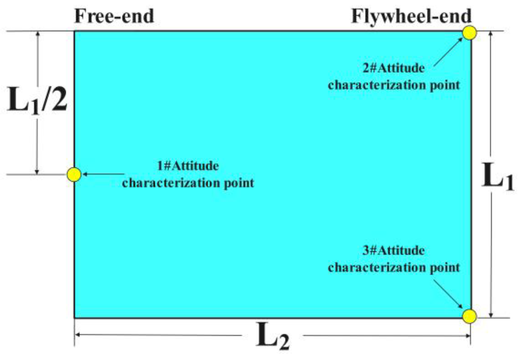
2.2.2. Characterization of the 6-DOF Attitude of the Main Engine

In the absence of degrees-of-freedom (DOF) constraints, the main engine can be regarded as a rigid body with 6 DOF. In this condition, the deflection of the main engine is zero, meeting the verification requirements. During the hoisting and positioning of the main engine, a full 6-DOF characterization of its attitude is required. By adjusting its rotational and translational degrees of freedom along the transverse (x-axis), longitudinal (y-axis), and vertical (z-axis) directions, the main engine shafting can be assembled into a straight line, ensuring that the GAP and SAG between the shafting connection flanges of the main engine meet the design specifications.

By arbitrarily defining a unit vector $\mathrm{n}=\left({\mathrm{n}}_{\mathrm{x}},{\mathrm{n}}_{\mathrm{y}},{\mathrm{n}}_{\mathrm{z}}\right)$ and a rotation angle $\theta$ in space, a rotation matrix R can be represented using the Rodrigues formula:

$$\mathrm{R}=\left[\begin{array}{ccc}\cos \theta +{\mathrm{n}}_{\mathrm{x}}^2\left(1-\cos \theta \right)& {\mathrm{n}}_{\mathrm{x}}{\mathrm{n}}_{\mathrm{y}}\left(1-\cos \theta \right)-{\mathrm{n}}_{\mathrm{z}}\sin \theta & {\mathrm{n}}_{\mathrm{x}}{\mathrm{n}}_{\mathrm{z}}\left(1-\cos \theta \right)+{\mathrm{n}}_{\mathrm{y}}\sin \theta \\ {\mathrm{n}}_{\mathrm{y}}{\mathrm{n}}_{\mathrm{x}}\left(1-\cos \theta \right)+{\mathrm{n}}_{\mathrm{z}}\sin \theta & \cos \theta +{\mathrm{n}}_{\mathrm{y}}^2\left(1-\cos \theta \right)& {\mathrm{n}}_{\mathrm{y}}{\mathrm{n}}_{\mathrm{z}}\left(1-\cos \theta \right)-{\mathrm{n}}_{\mathrm{x}}\sin \theta \\ {\mathrm{n}}_{\mathrm{z}}{\mathrm{n}}_{\mathrm{x}}\left(1-\cos \theta \right)-{\mathrm{n}}_{\mathrm{y}}\sin \theta & {\mathrm{n}}_{\mathrm{z}}{\mathrm{n}}_{\mathrm{y}}\left(1-\cos \theta \right)+{\mathrm{n}}_{\mathrm{x}}\sin \theta & \cos \theta +{\mathrm{n}}_{\mathrm{z}}^2\left(1-\cos \theta \right)\end{array}\right]$$

(1)

The three rotational degrees of freedom are extracted from $\mathrm{R}$, namely the rotation about the x-axis by ${\theta }_x$, rotation about the y-axis by ${\theta }_y$, and rotation about the z-axis by ${\theta }_z$:

$$\left\{\begin{array}{c}{\theta }_{\mathrm{x}}=\mathrm{a}\mathrm{r}\mathrm{c}\mathrm{t}\mathrm{a}\mathrm{n}2\left({\mathrm{R}}_{32},{\mathrm{R}}_{33}\right) \\ {\theta }_{\mathrm{y}}=\mathrm{a}\mathrm{r}\mathrm{c}\mathrm{s}\mathrm{i}\mathrm{n}\left(-{\mathrm{R}}_{31}\right)\\ {\theta }_{\mathrm{z}}=\mathrm{a}\mathrm{r}\mathrm{c}\mathrm{t}\mathrm{a}\mathrm{n}2\left({\mathrm{R}}_{21},{\mathrm{R}}_{11}\right)\end{array}\right.$$

(2)

In the formula, ${\mathrm{R}}_{11},{ \mathrm{R}}_{21},{ \mathrm{R}}_{31},{ \mathrm{R}}_{32},{ \mathrm{R}}_{33}$ are elements of $\mathrm{R}$. For example, ${\mathrm{R}}_{21}$ is the element in the second row and first column of $\mathrm{R}$.

By combining the three translational degrees of freedom, displacement along the x-axis by $\Delta \mathrm{x}$, along the y-axis by $\Delta \mathrm{y}$, and along the z-axis by $\Delta \mathrm{z}$, the 6-DOF attitude of the main engine can be characterized. By calculating the GAP and SAG between the connection flanges under different attitudes, the initial hoisting and positioning of the main engine can be guided [23]. A schematic diagram of the 6 DOF of the main engine is shown in Figure 3.

2.2.3. Characterization of the 3-DOF Attitude of the Main Engine

After the preliminary hoisting and positioning of the main engine in marine propulsion systems with single stern tube bearing, the GAP and SAG meet the design specifications. Therefore, the transverse and longitudinal positions of the main engine are no longer adjusted and the displacement in these two directions will be constrained. Only the vertical heights of the free end and flywheel end of the main engine are adjusted. When adjusting the main engine, care should be taken to avoid excessive deflection after adjustment. It is necessary to ensure that the characterized attitudes meet the factory inspection requirements for flatness, twist, and parallelism. To achieve this, the three-point plane positioning principle can be used to characterize the attitude of the main engine.

Two planes are defined by three points in space, $\left({\mathrm{x}}_{\mathrm{i}},{\mathrm{y}}_{\mathrm{i}},{\mathrm{z}}_{\mathrm{i}}\right)$ and $\left({\mathrm{x}}_{\mathrm{i}},{\mathrm{y}}_{\mathrm{i}},{{\mathrm{z}}_{\mathrm{i}}}^{\prime }\right)$, i = 1, 2, 3, and the normal vectors of these planes are calculated using the following formula:

$$\left\{\begin{array}{c}{\overrightarrow{\mathrm{N}}}_1=\left|\begin{array}{ccc}\mathrm{i}& \mathrm{j}& \mathrm{k}\\ {\mathrm{x}}_2-{\mathrm{x}}_1& {\mathrm{y}}_2-{\mathrm{y}}_1& {\mathrm{z}}_2-{\mathrm{z}}_1\\ {\mathrm{x}}_3-{\mathrm{x}}_1& {\mathrm{y}}_3-{\mathrm{y}}_1& {\mathrm{z}}_3-{\mathrm{z}}_1\end{array}\right|\\ {\overrightarrow{\mathrm{N}}}_2=\left|\begin{array}{ccc}\mathrm{i}& \mathrm{j}& \mathrm{k}\\ {\mathrm{x}}_2-{\mathrm{x}}_1& {\mathrm{y}}_2-{\mathrm{y}}_1& {{\mathrm{z}}_2}^{\prime }-{{\mathrm{z}}_1}^{\prime }\\ {\mathrm{x}}_3-{\mathrm{x}}_1& {\mathrm{y}}_3-{\mathrm{y}}_1& {{\mathrm{z}}_3}^{\prime }-{{\mathrm{z}}_1}^{\prime }\end{array}\right|\end{array}\right.$$

(3)

Using the components of the normal vectors, the projection normal vectors of the two planes onto the x–y plane are calculated. It can be observed that the two projection normal vectors are linearly related and the correlation coefficient is $\mathrm{K}$:

$$\overrightarrow{{\mathrm{N}}_{1\mathrm{xy}}}=\mathrm{K}\times \overrightarrow{{\mathrm{N}}_{2\mathrm{xy}}}$$

(4)

Therefore, when only the vertical heights of the three points are changed, the resulting different planes coincide in their projection onto the x–y plane and, under this constraint, the main engine retains only three degrees of freedom: rotation about the x-axis by ${\theta }_x$, rotation about the y-axis by ${\theta }_y$, and displacement along the z-axis by $\Delta \mathrm{z}$. Three non-collinear points at the bottom of the main engine are selected as attitude characterization points, serving as adjustment parameters. By designing different vertical heights for these three points, various planes at the bottom of the main engine can be formed, thereby characterizing different 3-DOF attitudes of the main engine.

Due to the concentrated mass at the flywheel end of the main engine, adjusting the jacking bolts closest to the flywheel end has the most significant impact on the verification parameters [24]. Therefore, the positions of the selected attitude characterization points are shown in Figure 4. L₁ is the main engine’s width and L₂ is its length.

2.2.4. Determination of the Actual Adjustment Parameters

To determine the actual adjustment parameters, the attitude of the main engine characterized by the attitude characterization points needs to be transformed through affine transformation to obtain the vertical adjustment amount of the jacking bolts [25]. The spatial coordinates of the attitude characterization points are $\left(x_{1i}, y_{1i}, z_{1i}\right)$, i = 1, 2, 3, and the augmented matrix $P$ is

$$\mathrm{P}=\left[ \begin{array}{cccc}{\mathrm{x}}_{11}& {\mathrm{y}}_{11}& {\mathrm{z}}_{11}& 1\\ {\mathrm{x}}_{12}& {\mathrm{y}}_{12}& {\mathrm{z}}_{12}& 1\\ {\mathrm{x}}_{13}& {\mathrm{y}}_{13}& {\mathrm{z}}_{13}& 1\end{array} \right]$$

(5)

Only the vertical height of the attitude characterization points is adjusted. The vertical height of the attitude characterization points is $z_{1i}$ before adjustment and ${z_{1i}}^{\prime }$ after adjustment, the vertical adjustment amount is $d_{1i}={z_{1i}}^{\prime }-z_{1i}$, and the target matrix $\mathrm{Q}$ can be approximated as

$$\mathrm{Q}=\left[ \begin{array}{ccc}{\mathrm{x}}_{11}& {\mathrm{y}}_{11}& {{\mathrm{z}}_{11}}^{\prime }\\ {\mathrm{x}}_{12}& {\mathrm{y}}_{12}& {{\mathrm{z}}_{12}}^{\prime }\\ {\mathrm{x}}_{13}& {\mathrm{y}}_{13}& {{\mathrm{z}}_{13}}^{\prime }\end{array} \right]$$

(6)

The affine transformation matrix $A$ is solved using the least squares method, which minimizes $\parallel PA-Q{\parallel }_2^2$:

$$\mathrm{A}={({\mathrm{P}}^{\mathrm{T}}\mathrm{P})}^{-1}{\mathrm{P}}^{\mathrm{T}}\mathrm{Q}$$

(7)

The coordinates of the jacking bolts before adjustment are $\left(x_{2i},y_{2i},z_{2i}\right)$, i = 1, 2, 3, 4 …… n, and, after obtaining the affine transformation matrix$A$, the adjusted coordinates of the jacking bolts $\left({x_{2i}}^{\prime },{{\mathrm{y}}_{2i}}^{\prime },{z_{2i}}^{\prime }\right)$ can be calculated with the following formula:

$$\left({{\mathrm{x}}_{2\mathrm{i}}}^{\prime },{{\mathrm{y}}_{2\mathrm{i}}}^{\prime },{{\mathrm{z}}_{2\mathrm{i}}}^{\prime }\right)=\left[ \begin{array}{cccc}{\mathrm{x}}_{2\mathrm{i}}& {\mathrm{y}}_{2\mathrm{i}}& {\mathrm{z}}_{2\mathrm{i}}& 1\end{array} \right]\mathrm{A}$$

(8)

The vertical adjustment amount of the jacking bolts is $d_{2i}={z_{2i}}^{\prime }-z_{2i}$ and the mapping relationship for the four jacking bolts is shown in Figure 5.

Finally, based on the 3-DOF attitude characterization of the main engine, the attitude is mapped to the vertical adjustment amounts of the jacking bolts, resulting in the development of an actual adjustment plan.

3. Alignment Method for Marine Propulsion Systems with Single Stern Tube Bearing Based on Fine-Tuning a Pre-Trained Model

The theme of this study innovatively applies the method of fine-tuning a pre-trained model to the alignment process of marine propulsion systems with single stern tube bearing, aims to achieve precise and efficient alignment to avoid friction and premature bearing failure caused by inaccurate alignment, and thereby can enhance the reliability and safety of ship navigation, reducing the failure rate and the risk of costly repairs. This study offers the potential for significant improvements in the alignment of propulsion systems and aligns with the current industry needs in the field of marine engineering.

3.1. Construction of the Functional Relationship Between Verification Parameters and Adjustment Parameters

The alignment of the propulsion system is a multi-objective constrained computational problem. Therefore, it is necessary to establish an accurate functional relationship between the verification parameters and adjustment parameters. Neural network models are a highly flexible and unbiased class of mathematical functions capable of approximating any real-valued function with arbitrary precision [26].

This research aims to address a specific gap in the field of propulsion system alignment. Traditional alignment methods for propulsion systems heavily rely on the knowledge and experience of construction personnel, which may lead to multiple alignments still failing to meet verification requirements. Moreover, traditional data-driven machine learning methods face the issue of time-consuming and inefficient collection of large-scale actual samples. Additionally, due to the parameter uncertainties in actual propulsion systems, it is not possible to establish an accurate functional relationship between the verification parameters and the adjustment parameters in the design of propulsion systems. To address the aforementioned problems, this paper proposes the application of a fine-tuning a pre-trained model method. In the small-sample scenario of the actual propulsion system alignment process, this method establishes an accurate functional relationship between the verification quantities and the adjustment quantities, thereby guiding the actual alignment and improving the accuracy and efficiency of the alignment process.

The overall concept is illustrated in Figure 6. First, large-scale samples are obtained through the finite element simulation of the design propulsion system and are used to construct a neural network model with prior knowledge which will serve as the pre-trained model for subsequent fine-tuning. This model represents the functional relationship between the verification parameters and adjustment parameters in the design propulsion system. Next, small samples are collected during the iterative alignment process of the actual propulsion system and used to fine-tune the pre-trained model. The resulting target model is then used to guide the next alignment in the iterative process. In this iterative process, along with the expansion of the target samples, the target model obtained by fine-tuning the pre-trained model will ultimately reflect the accurate functional relationship between the verification parameters and adjustment parameters in the actual propulsion system.

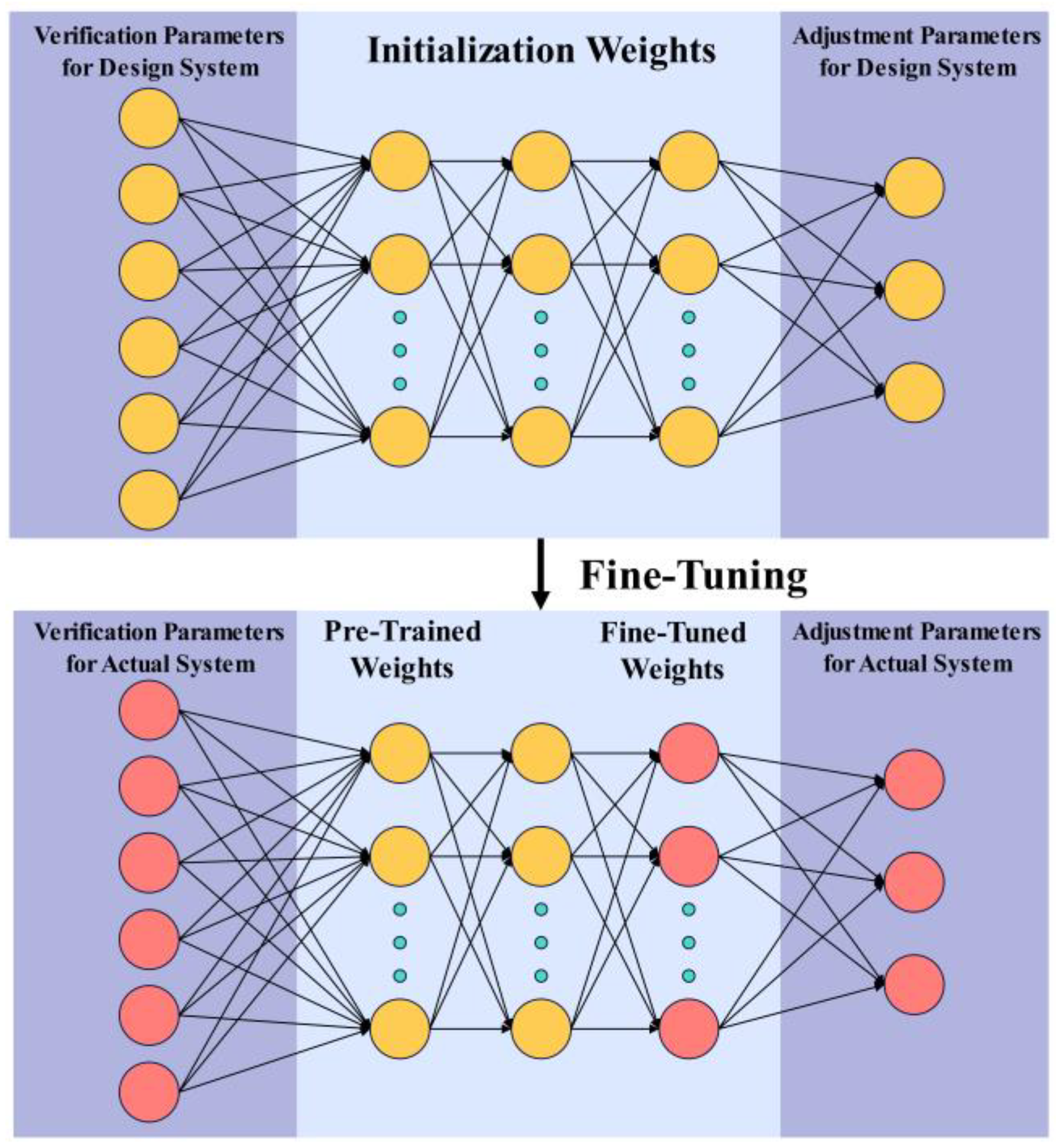
3.2. Pre-Training and Fine-Tuning Learning Paradigm

The pre-training and fine-tuning learning paradigm has been applied to problems with incomplete information [27,28]. First, a pre-trained model is built using large-scale samples, allowing for the extensive learning of prior knowledge; then, fine-tuning is performed in downstream tasks, avoiding the need to train a model from scratch for the downstream tasks. This approach is particularly suited for data-scarce situations and can significantly improve the model’s performance on downstream tasks. The method strategy is shown in Figure 7. First, the weights of the early layers of the pre-trained model are frozen and then the weights of the later layers are retrained [29]. The early layers of the model extract general features, while the later layers focus on features specific to the task. Freezing the early layers and fine-tuning the later layers allows the model to concentrate on learning features specific to the particular task. Moreover, freezing the parameters of the early layers reduces the number of parameters that need to be updated, thereby decreasing the complexity of the model. This is conducive to reducing the risk of overfitting and enhancing the model’s generalization capability.

3.3. Construction of the Pre-Trained Model

3.3.1. Topology of the BP Neural Network

Back Propagation (BP) neural networks, which have the basic principle of calculating their output through forward propagation, then computing the error gradients using a back propagation algorithm, and finally updating the network weights according to the gradients, thereby continuously optimizing the model parameters, have strong feature extraction and learning capabilities and have been successfully applied in the alignment of propulsion systems [30]. Compared to the potential model Radial Basis Function (RBF) neural networks, which may be applicable to the alignment problem of propulsion systems, a BP neural network, through the back propagation algorithm, offers stronger adaptability and capability in handling global issues. The basic network structure consists of three hidden layers. The inputs are the crankshaft vertical deflection of the n# cylinder, the crankshaft horizontal deflection of the n# cylinder, the intermediate bearing load, and the thrust bearing load, both before and after the adjustment of the main engine. The outputs are three dimensions, representing the adjustment amounts of three attitude characterization points. This is shown in Figure 8.

The evaluation metrics for the fitting quality of the pre-trained model are the coefficient of determination ${\mathrm{R}}^2$, mean absolute error ($\mathrm{MAE}$), and root mean square error ($\mathrm{RMSE}$):

$${\mathrm{R}}^2=1-\left({{\displaystyle \sum }}_{\mathrm{i}=1}^{\mathrm{n}}{\left({\mathrm{y}}_{\mathrm{i}}-{\mathrm{y}}_{\mathrm{i},\mathrm{pred}}\right)}^2/{{\displaystyle \sum }}_{\mathrm{i}=1}^{\mathrm{n}}{\left({\mathrm{y}}_{\mathrm{i}}-\bar{\mathrm{y}}\right)}^2\right)$$

(9)

$$\mathrm{MAE}={\displaystyle \frac{1}{\mathrm{n}}}{{\displaystyle \sum }}_{\mathrm{i}=1}^{\mathrm{n}}\left|{\mathrm{y}}_{\mathrm{i}}-{\mathrm{y}}_{\mathrm{i},\mathrm{pred}}\right|$$

(10)

$$\mathrm{RMSE}=\sqrt{{\displaystyle \frac{1}{\mathrm{n}}}{{\displaystyle \sum }}_{\mathrm{i}=1}^{\mathrm{n}}{\left({\mathrm{y}}_{\mathrm{i}}-{\mathrm{y}}_{\mathrm{i},\mathrm{pred}}\right)}^2}$$

(11)

In the formula, ${\mathrm{y}}_{\mathrm{i}},{ \mathrm{y}}_{\mathrm{i},\mathrm{pred}}, \bar{\mathrm{y}}$ represent the true value of the ith sample, the predicted value of the ith sample, and the average of the true values and n is the number of samples.

3.3.2. Acquisition of Training Samples

To acquire training samples, it is necessary to reasonably design a sampling scheme based on the vertical heights of attitude characterization points on the same reference horizontal plane, in order to calculate the values of verification parameters under different attitudes of the main engine. Based on the actual engineering adjustment range and unit adjustment amount, the vertical height sampling range and precision at the attitude characterization points are determined. For the three attitude characterization points, the number of sample features is 3.

In order to ensure the establishment of an effective pre-trained model, a balanced dataset with sample distribution is required for neural network training. The Latin Hypercube Sampling (LHS) method and traditional Random Sampling (RS) method are used to generate the same number of samples. By plotting cumulative distribution function (CDF) comparison charts, the distribution characteristics among the three sample features in the dataset can be illustrated. The Empirical CDF (ECDF) is the function based on the generated samples, while the Uniform CDF (UCDF) is the theoretical cumulative distribution function for a uniform distribution; the vertical height sampling range at the attitude characterization points is from $\mathrm{m}$ to $\mathrm{M}$, so the domain of the function is $\mathrm{x}\in \left[\mathrm{m},\mathrm{M}\right]$. The function formula is as follows:

$$\mathrm{ECDF}\left(\mathrm{x}\right)={\displaystyle \frac{1}{\mathrm{n}}}{{\displaystyle \sum }}_{\mathrm{i}=1}^{\mathrm{n}}\mathrm{I}\left({\mathrm{x}}_{\mathrm{i}}\le \mathrm{x}\right) \mathrm{while} \mathrm{I}\left({\mathrm{x}}_{\mathrm{i}}\le \mathrm{x}\right)=1, \mathrm{when} {\mathrm{x}}_{\mathrm{i}}\le \mathrm{x}$$

(12)

$$\mathrm{UCDF}\left(\mathrm{x}\right)=\left(\mathrm{x}-\mathrm{m}\right)/\left(\mathrm{M}-\mathrm{m}\right)$$

(13)

In Formula (12), n is the number of samples and ${\mathrm{x}}_{\mathrm{i}}$ is the value of the ith sample.

By comparing the ECDF and UCDF of the three sample features generated by the two sampling methods in Figure 9, in the figure, it is assumed that the sampling range of all three sample features is between −2 and 2, it can be observed that the LHS ensures that the samples are uniformly distributed across each dimension. Even with a limited sample size, LHS can more effectively estimate the characteristics of the parameter space. Compared to RS, LHS avoids issues such as incomplete sampling coverage and redundancy and it ensures better representativeness, especially when sampling in high-dimensional spaces [31]. Therefore, LHS is used for sampling in this research.

3.3.3. Data Processing of Training Samples

The sample set generated by LHS sampling consists of n samples, representing n different attitudes of the main engine. The values of the verification parameters at different attitudes are obtained through finite element simulations. As shown in Figure 10, by calculating the vertical height difference between attitude characterization points in any two samples, the vertical adjustment of the attitude characterization points can be determined, the values of the verification parameters before and after the adjustment are then combined, forming a training sample for training the neural network.

In training the neural network, to eliminate the scale differences between sample features, a normalization technique is often used to make the sample dimensionless. In this research, the commonly used Min–Max Normalization is chosen, which linearly transforms the training samples to the range [0, 1]. The formula is as follows:

$${{\mathrm{x}}_{\mathrm{i}}}^{\prime }=\left({\mathrm{x}}_{\mathrm{i}}-\underset{1\le \mathrm{j}\le \mathrm{n}}{\min }\left\{{\mathrm{x}}_{\mathrm{j}}\right\}\right)/\left(\underset{1\le \mathrm{j}\le \mathrm{n}}{\max }\left\{{\mathrm{x}}_{\mathrm{j}}\right\}-\underset{1\le \mathrm{j}\le \mathrm{n}}{\min }\left\{{\mathrm{x}}_{\mathrm{j}}\right\}\right)$$

(14)

3.4. Construction of the Target Small-Sample Dataset

3.4.1. Target Measured Samples

The target measured samples will gradually expand with the iterative process of the propulsion system alignment. This includes (1) the adjustment amounts of the attitude characterization points predicted by the neural network, when the actual values of each verification parameter and the designed values are input into the neural network. (2) After mapping to the adjustment amount of the jacking bolts and performing the adjustment, the bearing load measured using the jack-up method, as well as the crankshaft deflection measured by placing a crankshaft deflection gauge at the measurement point between the crank arms, are recorded; the distance from the measurement point to the centerline of the crankshaft journal is $\left(\mathrm{S}+\mathrm{D}\right)/2$, where $\mathrm{S}$ is the stroke length of the diesel engine piston and $\mathrm{D}$ is the diameter of the main journal [32]. The alignment process from the shipyard survey is shown in Figure 11.

[d₁n,d₂n,d₃n] represent the adjustment amounts of the attitude characterization points at the nth alignment, while [f₁n,f₂n,f₃n,f₄n] represent the values of the verification parameters before the nth alignment and [f₁0,f₂0,f₃0,f₄0] represent the design values of the verification parameters.

During the first alignment, when there is no target measured sample for fine-tuning, the pre-trained model is used to predict the adjustment amounts for the main engine attitude characterization points. The pre-trained model input is [f₁1,f₂1,f₃1,f₄1,f₁0,f₂0,f₃0,f₄0], and the pre-trained model output is [d₁1,d₂1,d₃1]. Then, the adjusted verification parameters values are measured as [f₁2,f₂2,f₃2,f₄2].

During the second alignment, a complete set of target measured sample is available, as shown in

Table 1. Composition of target measured samples.

Number of Alignments	Adjustment Parameters	Verification Parameters	Target Measured Samples
0	\	[f11,f21,f31,f41]	\
1	[d11,d21,d31]	[f12,f22,f32,f42]	[f11,f21,f31,f41,f12,f22,f32,f42;d11,d21,d31]
2	[d12,d22,d32]	[f13,f23,f33,f43]	[f12,f22,f32,f42,f13,f23,f33,f43;d12,d22,d32]

with the data [f₁1,f₂1,f₃1,f₄1,f₁2,f₂2,f₃2,f₄2;d₁1,d₂1,d₃1]. At this point, the pre-trained model can be fine-tuned using the target measured sample to obtain the target model, which will guide the next main engine adjustment. The target model input is [f₁2,f₂2,f₃2,f₄2,f₁0,f₂0,f₃0,f₄0] and the target model output is [d₁2,d₂2,d₃2].

3.4.2. Data Augmentation

The method of expanding one target measured sample after each iterative adjustment and fine-tuning the pre-trained model is inefficient and results in a limited sample size. As a result, the target model struggles to comprehensively learn the target knowledge and is prone to overfitting the small amount of target samples. Using data augmentation techniques can increase the diversity of the small-sample dataset, covering more actual alignment scenarios of the propulsion system, thereby improving the generalization ability and robustness of the target model.

Two samples are randomly selected from the existing small-sample dataset and combined to generate a new sample in order to ensure that the functional relationship between the verification parameters and the adjustment parameters is not altered in the new samples after data augmentation. By swapping the values of the verification parameters before and after the adjustment and take the opposite of the adjustment amounts for the attitude characterization points, another new sample is obtained. If the number of adjustments is n, the sample size in the small-sample dataset before data augmentation should be n. After data augmentation using the feature combination method, the sample size in the augmented dataset can be calculated as follows:

$$\mathrm{A}\left(\mathrm{n}+1,2\right)={\displaystyle \frac{\left(\mathrm{n}+1\right)!}{\left(\mathrm{n}+1-2\right)!}}=\left(\mathrm{n}+1\right)\times \mathrm{n}$$

(15)

The final dataset obtained after data augmentation is the target small-sample dataset and the data augmentation method is shown in

Table 2. Small-sample dataset before and after data augmentation.

Number of Alignments	Before Data Augmentation	After Data Augmentation
1	(1) [f11,f21,f31,f41,f12,f22,f32,f42;d11,d21,d31]	(1) [f11,f21,f31,f41,f12,f22,f32,f42;d11,d21,d31] (2) [f12,f22,f32,f42,f11,f21,f31,f41;−d11,−d21,−d31]
2	(1) [f11,f21,f31,f41,f12,f22,f32,f42;d11,d21,d31] (2) [f12,f22,f32,f42,f13,f23,f33,f43;d12,d22,d32]	(1) [f11,f21,f31,f41,f12,f22,f32,f42;d11,d21,d31] (2) [f12,f22,f32,f42,f13,f23,f33,f43;d12,d22,d32] (3) [f11,f21,f31,f41,f13,f23,f33,f43;d11+d12,d21+d22,d31+d32] (4) [f12,f22,f32,f42,f11,f21,f31,f41;−d11,−d21,−d31] (5) [f13,f23,f33,f43,f12,f22,f32,f42;−d12,−d22,−d32] (6) [f13,f23,f33,f43,f11,f21,f31,f41;−(d11+d12),−(d21+d22),−(d31+d32)]

.

In the actual object iterative alignment process, it is necessary to construct the data-augmented target small-sample dataset D_n for fine-tuning the pre-trained model, where n represents the alignment iteration number. This results in a target model to guide the n + 1th alignment. During the iterative process, applying data augmentation strategies without altering the model structure can increase sample diversity. As a result, this reduces the risk of model overfitting and enables the model to stabilize more quickly at a high performance level during the training process.

4. Application Example

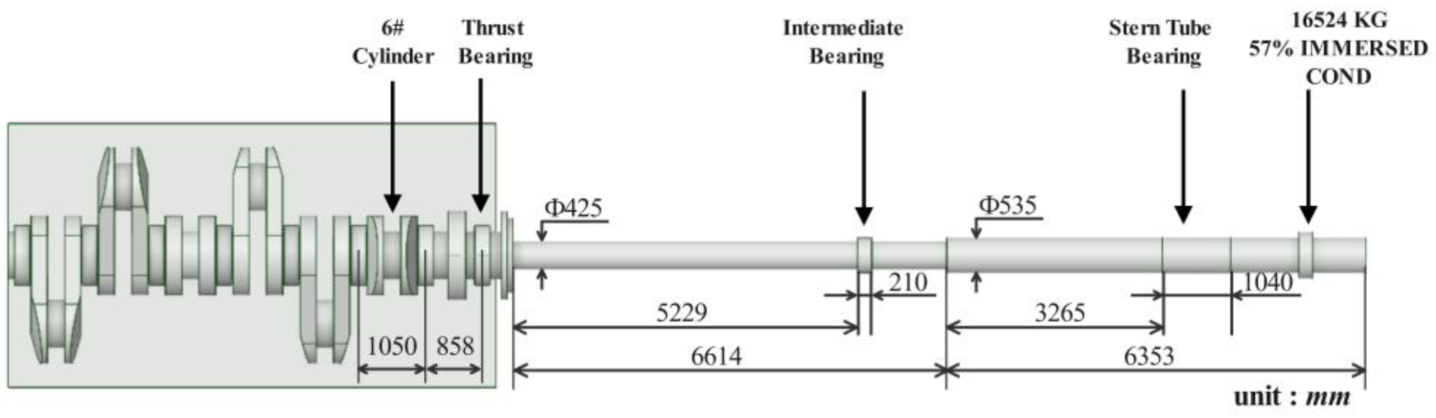
4.1. Research Object

The research object is the propulsion system shown in Figure 12. The shafting in the propulsion system has a total length of 12,967 mm, with the intermediate shaft length being 6614 mm, and it is supported by a single intermediate bearing. The propeller shaft is 6353 mm and the stern tube has no forward stern tube bearing. The main engine in the propulsion system is a 6-cylinder model 6S60MC diesel engine equipped with four jacking bolts at the bottom.

The geometric model of the propulsion system is constructed based on the design parameters from the drawings. Using ANSYS 2023R1 finite element software and under the condition of the propeller being 57% immersed, a numerical model is established based on the physical parameters provided in the calculation sheet. The specific parameters are as follows: the weight of the propeller at 57% immersion is 16,524 kg, the mass of the turning wheel is 12,363 kg, the chain force acting on the thrust shaft is 108,600 N, and the reciprocating mass per cylinder of the crankshaft is 4541 kg. This model is defined as the design object.

The actual object is based on the design object, taking into account the actual existing compound deviation factors. These deviations arise from the parameter uncertainties in the construction of the geometric and numerical models. For example, the actual weight of the main engine may deviate from the design weight due to design errors or the impact of anti-corrosion coating materials. The actual material stiffness of the main engine may decrease over time compared to the design value due to prolonged operation in harsh environments. The relative slope between the stern tube bearing and the shaft may also deviate from the design slope due to installation process errors.

In this section, the deviation factors in

Table 3. Propulsion System Deviation Factors.

Deviation Type	Deviation Factors
Main Engine Deviation	Main engine weight + 2% Main engine material stiffness − 10%
Shafting Deviation	The relative slope between the stern tube bearing and the shaft + 0.1 mm/m

are comprehensively considered in the finite element software to construct the numerical model of the target domain propulsion system, defined as the actual object. The subsequent work involves simulating the actual alignment process for this actual object by combining finite element simulations with fine-tuning the pre-trained model method, to verify the superiority of the proposed method.

4.2. Application of the Proposed Method in the Actual Object Alignment Process

4.2.1. Fine-Tuning Strategy

The pre-trained fine-tuning strategy in this paper selects to freeze all layers of the pre-trained model except for the last layer and only fine-tunes the weights of the last layer, transferring the prior knowledge learned by the earlier layers to the downstream task.

4.2.2. Construction of the Pre-Trained Model

Sampling is performed using LHS, with the vertical height of the attitude characterization points sampled within the range of [−2 mm, 2 mm] and a sampling precision of 0.01 mm. Based on this, a sample set of 2000 samples, each with 3 features, is constructed. Finite element simulation is used to calculate the verification parameter values for 2000 different attitudes of the main engine in the design object. After preprocessing the generated data, 1800 samples are used for training the neural network to establish the pre-trained model, which will be used in the subsequent analysis. The network structure parameters are shown in

Table 4. Pre-trained model parameters.

Network Parameters	Parameter Values	Network Parameters	Parameter Values
Number of Network Layers	5	Training/Test/Validation	0.8/0.1/0.1
Number of Input Neurons	8	Epoch	5000
Number of Output Neurons	3	Activation Function	ReLU
Number of Hidden Layers	3	Optimization Algorithm	Adam

. Additionally, 200 samples are used for testing to validate the performance metrics of the pre-trained model, with the results shown in

Table 5. Performance of the pre-trained model.

Model Performance Evaluation Metrics	${\mathbf{R}}^2$	MAE	RMSE
Convergence Value	0.99	0.0021	0.0039

. Under the condition of 2000 samples, this division ratio is to ensure that the pre-trained model can learn enough prior knowledge and ensure that the pre-trained model can obtain a target model with high precision after fine-tuning in downstream tasks. As shown in Table 5, the high performance of the pre-trained model makes it possible to maintain good performance on the new task after appropriate fine-tuning.

4.2.3. Application Effect of the Proposed Method

According to the specifications of the main engine adjustment installation procedure and the shafting alignment calculation document, the allowable error range for the load of the intermediate bearing relative to the design value is within 20% in the actual factory inspection. The thrust bearing load should be as close as possible to the design value. The absolute values of the vertical deflection and the horizontal deflection of the 6# cylinder crankshaft should not exceed 0.33 mm in practice.

To improve the accuracy of the propulsion system alignment results, the expected relative error of the bearing loads compared to the design values should be within 5% and the expected absolute values of the crankshaft deflection should be within 0.05 mm. In the iterative alignment of the actual object, when all verification parameters meet the desired accuracy, the alignment is stopped. The trends of the relative error of the bearing loads and the absolute value of the crankshaft deflection are shown in Figure 13.

An analysis of Figure 13 shows that after the first alignment, the errors of each verification parameter are much larger than the desired final error, indicating that using the pre-trained model to guide the actual alignment is not effective. The reason for this is the significant discrepancies between the design object and the actual object.

During the initial alignment process, the errors of each verification parameter fluctuate significantly. This is because the target sample size is limited and the current model has learned only a small amount of feature knowledge, which is insufficient to effectively transfer the prior knowledge from the pre-trained model and combine it with the characteristics of the target to build a more adaptive target model. It is necessary to continue the iterative alignment process to expand the target sample size in order to increase the diversity of the sample features.

As the iterative alignment process progresses, the variation in verification parameter errors becomes stable, indicating that the sample size is sufficient to learn the target feature knowledge. By combining this with the prior knowledge from the pre-trained model, an accurate target model can be obtained.

After the 8th alignment, the error of each verification parameter had significantly decreased, and the accuracy and efficiency of the alignment process were greatly enhanced. The average errors of each verification parameter in the last three iterations of the alignment process are as follows: the relative errors are 3.4% for the thrust bearing load and 1.3% for the intermediate bearing load and the absolute values are 0.05 mm for the crankshaft vertical deflection of the 6# cylinder and 0.02 mm for the crankshaft horizontal deflection of the 6# cylinder; these results meet the expected alignment requirements and the alignment task has been completed. After 16 iterations, the current data-augmented target small-sample dataset, D₁₆, was obtained.

In summary, the good application effect of the proposed method in the alignment of the propulsion system was demonstrated through finite element simulations.

5. Discussion

This section is based on the design object, actual object, pre-trained model, and target small-sample dataset D₁₆ constructed in Section 4, combined with measured data recorded during field investigations at the shipyard; these data, obtained through the trial-and-error method guiding the alignment of the propulsion system (specific adjustment work shown in Figure 11), are further discussed.

(1)

Validating the effectiveness of the proposed method with actual measured data.

Based on the actual conditions of the shipyard, three trial-and-error alignments were performed by mapping the adjustment amounts of arbitrary attitude characterization points to the jacking bolts. During the trial-and-error process, conducted three times, the variations in the errors of the verification parameters were irregular and could not be brought within the maximum allowable error range. The corresponding measured data, referred to as the target actual measured samples, were recorded to validate the effectiveness of the proposed method. The data from the second alignment were used to construct an actual measured sample dataset with a sample size of 1 and the data from the first and second alignments were used to construct an actual measured sample dataset with a sample size of 2. These datasets, representing different target small-sample datasets, were used to fine-tune the pre-trained model, resulting in different target models. Here, the adjustment parameters for the third alignment of the main engine are predicted based on different target models and the predicted adjustment amounts of the attitude characterization points are constructed into the adjustment parameter matrix. To evaluate the model’s prediction accuracy, the Euclidean Distance Similarity (EDS) and Cosine Similarity (CS) are used to compare and analyze the similarity between the predicted adjustment parameter matrix and the actual adjustment parameter matrix. For two matrices A and B with the same dimensions of $\mathrm{m}\times \mathrm{n}$, the formulas for calculating the EDS and CS are as follows:

$$\mathrm{EDS}\left(\mathrm{A},\mathrm{B}\right)={\displaystyle \frac{1}{1+\sqrt{{{\displaystyle \sum }}_{\mathrm{i}=1}^{\mathrm{m}}{{\displaystyle \sum }}_{\mathrm{j}=1}^{\mathrm{n}}{\left({\mathrm{A}}_{\mathrm{ij}}-{\mathrm{B}}_{\mathrm{ij}}\right)}^2}}}$$

(16)

$$\mathrm{CS}\left(\mathrm{A},\mathrm{B}\right)={\displaystyle \frac{{{\displaystyle \sum }}_{\mathrm{i}=1}^{\mathrm{m}}{{\displaystyle \sum }}_{\mathrm{j}=1}^{\mathrm{n}}{\mathrm{A}}_{\mathrm{ij}}\cdot {\mathrm{B}}_{\mathrm{ij}}}{\sqrt{{{\displaystyle \sum }}_{\mathrm{i}=1}^{\mathrm{m}}{{\displaystyle \sum }}_{\mathrm{j}=1}^{\mathrm{n}}{\mathrm{A}}_{\mathrm{ij}}^2}\cdot \sqrt{{{\displaystyle \sum }}_{\mathrm{i}=1}^{\mathrm{m}}{{\displaystyle \sum }}_{\mathrm{j}=1}^{\mathrm{n}}{\mathrm{B}}_{\mathrm{ij}}^2}}}$$

(17)

The EDS analyzes the absolute difference in the numerical distribution between matrices, with a value range from 0 to 1. The CS analyzes the relative positional similarity between matrices, with a value range from −1 to 1. When both similarities are equal to 1, it indicates that the two matrices are identical, meaning the model’s predicted results are exactly the same as the actual results. Figure 14 compares the changes in similarity between the adjustment parameter matrix predicted by the models obtained using different actual measured sample sizes combined with the proposed method and the actual adjustment parameter matrix.

As shown in Figure 14, with the increase in the measured sample size, the similarity between the adjustment parameter matrix predicted by the target model and the actual adjustment parameter matrix significantly improves. Compared to the similarity between the adjustment parameter matrix predicted by the pre-trained model and the actual adjustment parameter matrix when the actual measured sample size is zero, the proposed method significantly enhances the prediction accuracy of the model. This result validates the effectiveness of this method.

(2)

Validating the effectiveness of the proposed method with finite element simulation.

In the actual object, a small-sample dataset T_train is generated through finite element simulations and it is incrementally expanded to construct different small-sample datasets, which are used to fine-tune the pre-trained model to obtain different target models. For example, the dataset T_train,20 represents a subset consisting of the first 20 samples from T_train. At the same time, large-scale samples are generated through finite element simulations in the actual object to form T_test. Finally, the mean absolute error of the target model obtained from T_train,N (N is the sample size from T_train) is calculated on T_test. The accuracy formula, derived from Formula (10), is as follows:

$$\mathrm{Accuracy}={\displaystyle \frac{1}{1+\mathrm{MAE}}}$$

(18)

The accuracy data calculated from the above formula are fitted using a nonlinear function. The fitting function and its results are shown in Figure 15.

By analyzing the derivative of the fitted function in Figure 15, it can be observed that when the sample size reaches 11, the model’s accuracy tends to converge, approaching 0.95. This indicates that, under the current deviation between the actual object and the design object, when the sample size is 11, the target model demonstrates high prediction accuracy on T_test. This is consistent with the phenomenon observed in Figure 13, where, starting from the 11th adjustment, the errors of each verification parameter gradually converge after the alignment process is guided by the target model. This result illustrates that, under the conditions of this study, when the target sample size is 11, the combination of feature knowledge from the sample and the prior knowledge from the pre-trained model allows the model to be sufficiently adapted to the downstream task. This result validates the effectiveness of the proposed method.

(3)

Validating the superiority of the proposed method through comparison with traditional machine learning.

To compare the applicability of the traditional machine learning method and the proposed method under the limitation of small samples in the target domain, a baseline model is trained using D₁₆ combined with the traditional machine learning method, while a target model is obtained by fine-tuning the pre-trained model using D₁₆ combined with the proposed method. A model comparison is shown in

Table 6. Comparison of different models.

Model Type	Training Data	Training Method	Source of Knowledge
Target Model	D16	Fine-tuning pre-trained model method	(1) Prior knowledge from the pre-trained model (2) Feature knowledge from the target small samples
Baseline Model	D16	Traditional BP neural network training method	Feature knowledge from the target small samples

. Both models are tested in the actual object’s unfamiliar alignment task and the results are shown in Figure 16.

From the analysis of Figure 16, it can be seen that the target model can adjust each verification parameter to within the desired accuracy range with just one adjustment. In contrast, the baseline model, limited by the current sample size, fails to fully learn the target knowledge for guiding the actual alignment task, resulting in significant deviations of the verification parameters from the expected values.

(4)

Comparison of the proposed method with previous research.

Compared with other published materials [8,30], the research object of this study is marine propulsion systems with single stern tube bearing, but most existing research and alignment methods focus on multi-support shafting. During the alignment process of marine propulsion systems with single stern tube bearing, only the engine attitude can be adjusted, thus requiring specialized alignment techniques. Unlike traditional alignment methods, this paper applies a model pre-trained in the design propulsion system field and fine-tunes it for specific alignment tasks in actual marine propulsion systems with single stern tube bearing. This research could pave the way for more automated alignment procedures, reducing human intervention and minimizing the potential for human error. The difference between the fine-tuning pre-trained model method proposed in this paper and Feng’s method [33] is that, due to the significant distribution differences of samples across different domains require adjusting the weight parameters of the first hidden layer, the parameter uncertainty in the actual object in this paper has a large impact on the sample values but little effect on the sample distribution. Therefore, in this research, only the last layer of the pre-trained model is re-trained, while the other layers are kept frozen to preserve the prior knowledge learned from large-scale samples for subsequent knowledge transfer. For tasks where there are significant distribution differences between the target samples and the source samples, the strategy proposed by Feng can be applied.

(5)

Future research directions.

This paper considers the impact of compound deviation factors to obtain the actual object. Future research could focus on alignment studies involving more deviation factors, such as different immersion states of the propeller. Future research could also explore pre-trained models under more complex network structures, such as Recurrent Neural Networks (RNNs), further improve the performance of the target model in the target task, and reduce the number of necessary iterations. Future research could explore the application of other data augmentation methods, such as the Synthetic Minority Oversampling Technique (SMOTE) and Generative Adversarial Networks (GANs), in fine-tuning pre-trained models and discuss how different data augmentation methods enhance the learning capabilities of the target model in specific tasks.

6. Conclusions

Currently, the alignment of marine propulsion systems with single stern tube bearing relies on manual trial-and-error, making it difficult to ensure the alignment’s accuracy and efficiency. Meanwhile, due to uncertainties in the actual parameters of propulsion systems and the limitations of small samples, the finite element simulation method and the traditional machine learning method struggle to effectively improve alignment accuracy and efficiency in practical applications. To address this, this paper proposes a method for characterizing the main engine attitude during alignment of marine propulsion systems with single stern tube bearing and introduces an alignment method for propulsion systems based on fine-tuning a pre-trained model. This method assumes that there is a correlation between the pre-training task and the downstream task and that the pre-training samples and target samples have similar sample distributions. The main conclusions are as follows:

• By using different combinations of vertical heights at the three attitude characterization points on the bottom of the main engine, the different attitudes of the main engine can be characterized when only the vertical heights of the free end and flywheel end of the main engine are adjusted.
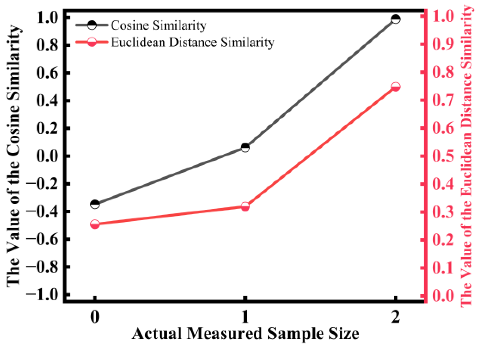
• The proposed method has been proven effective in small-sample scenarios, as validated by actual measured data. As the number of measured data increases, the variation in target models derived from the measured data leads to different predicted adjustment parameter matrices, while the similarity between these matrices and the actual adjustment parameter matrix continuously improves. Specifically, the Cosine Similarity increases from −0.35 to 0.98 and the Euclidean Distance Similarity increases from 0.26 to 0.75.
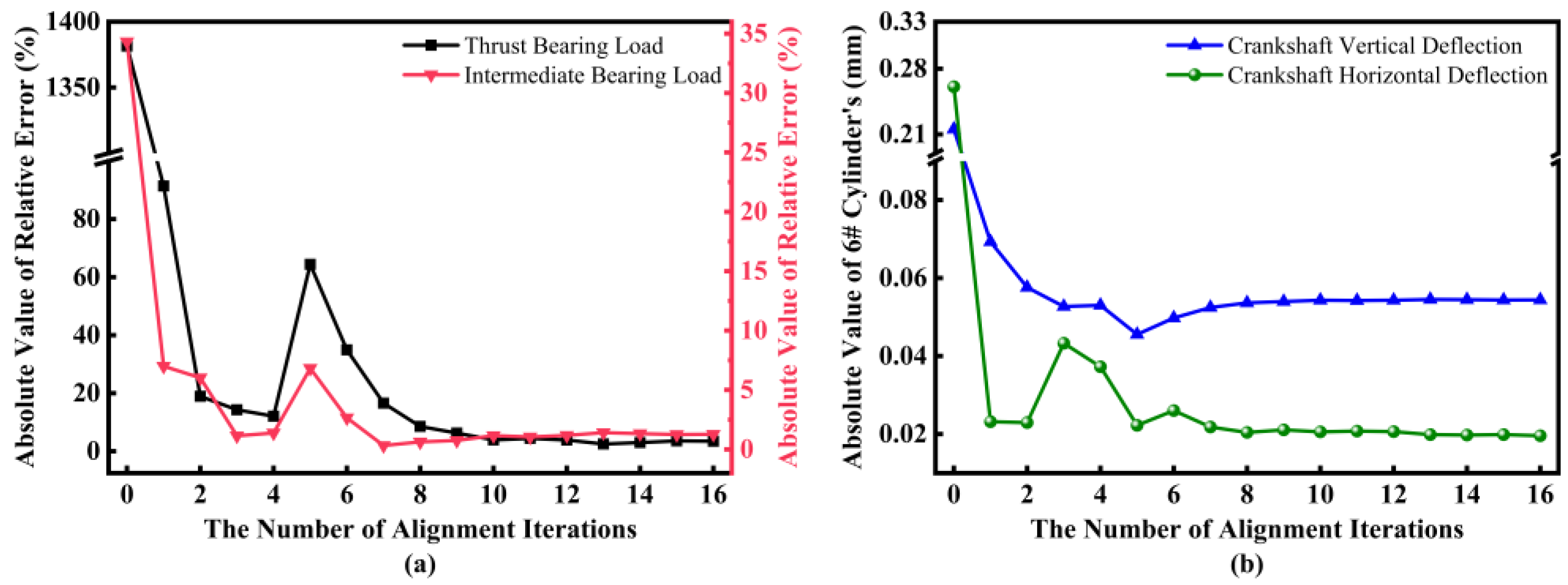
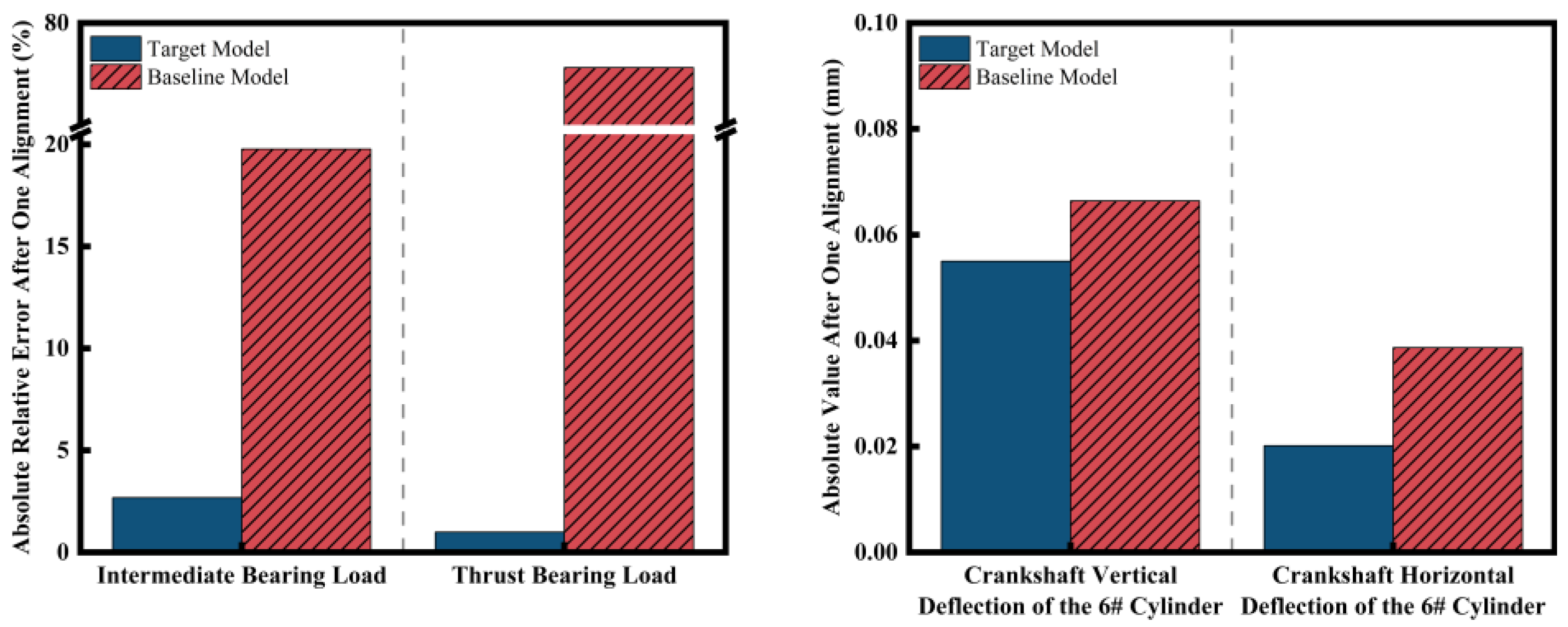
• Considering the uncertainties in propulsion system parameters, we constructed an actual alignment example using finite element simulation which validated the superiority of the proposed method. With only eight alignment iterations, the relative errors of the intermediate bearing load and thrust bearing load were 1.3% and 3.4%, respectively, significantly lower than the maximum error requirement of 20%. Additionally, the absolute values of the crankshaft vertical deflection and crankshaft horizontal deflection for the 6# cylinder were 0.05 mm and 0.02 mm, respectively, significantly lower than the maximum error requirement of 0.33 mm. Compared to manual alignment, where the alignment duration and precision are uncertain, the proposed method can ensure that the alignment precision is sufficiently high after only a few alignment iterations.
• The target model obtained through the proposed method achieved significant improvements over the baseline model obtained through the traditional machine learning method in the actual alignment example constructed in this study. Specifically, under the same alignment task, the relative errors of the intermediate bearing load and thrust bearing load decreased by 17.1% and 76.8%, respectively, while the absolute values of the crankshaft vertical deflection and crankshaft horizontal deflection for the 6# cylinder were reduced by 0.01 mm and 0.02 mm, respectively.

A limitation of this study is that it does not conduct comparative research on more complex network structures and other data augmentation methods. Therefore, future research should focus on the aforementioned limitations.

References

1. Lai, G.; Liu, J.; Liu, S.; Zeng, F.; Zhou, R.; Lei, J. Comprehensive optimization for the alignment quality and whirling vibration damping of a motor drive shafting. Ocean. Eng. 2018, 157, 26–34. [Google Scholar] [CrossRef]
2. Diego, L.M.; Dionísio, H.C.; Brenno, M.C.; Luiz, A.V.; Ulisses, A.M.; Ricardo, H.R. Machine learning performance comparison for main propulsive shafting systems alignment. Ocean. Eng. 2023, 280, 114556. [Google Scholar]
3. Zou, D.; Jiao, C.; Ta, N.; Rao, Z. Forced vibrations of a marine propulsion shafting with geometrical nonlinearity (primary and internal resonances). Mech. Mach. Theory 2016, 105, 304–319. [Google Scholar] [CrossRef]
4. Yang, Y.; Tang, W.; Che, C. Shafting Alignment based on Improved Three-moment Method with Hydrodynamic Simulation for Twin Propulsion Systems. J. Ship Mech. 2013, 17, 1038–1053. [Google Scholar]
5. Zhou, R.; Yao, S.; Zhang, S.; Li, B. Theoretic studies of the three-moment equation and its application in the vessel’s propulsion shafting alignment. J. Wuhan Univ. Technol. 2005, 27, 77–78. [Google Scholar]
6. Kandouci, C.; Adjal, Y. Forced Axial and Torsional Vibrations of a Shaft Line Using the Transfer Matrix Method Related to Solution Coefficients. J. Mar. Sci. Appl. 2014, 13, 200–205. [Google Scholar]
7. Wang, J.; Lou, J.; Li, X.; Chen, R. Research on the shafting alignment calculation based on differential equations for beam deformation and singularity functions. Ship Sci. Technol. 2019, 41, 71–75. [Google Scholar]
8. Deng, Y.; Yang, X.; Huang, Y.; Pan, T.; Zhu, H. Calculation Method of Intermediate Bearing Displacement Value for Multi-supported Shafting Based on Neural Network. J. Ship Res. 2021, 65, 286–292. [Google Scholar]
9. Zhang, Z.; Ma, X.; Yu, H.; Hua, H. Stochastic dynamics and sensitivity analysis of a multistage marine shafting system with uncertainties. Ocean Eng. 2020, 219, 108388. [Google Scholar] [CrossRef]
10. Lu, L.; Li, G.; Xing, P.; Gao, H.; Song, Y. A review of stochastic finite element and nonparametric modelling for ship propulsion shaft dynamic alignment. Ocean Eng. 2023, 286, 115656. [Google Scholar] [CrossRef]
11. Gong, T. Process Control for Long Shafting Construction Quality and Period on High-Tech New Naval Ship. Master’s Thesis, Shanghai Jiao Tong University, Shanghai, China, 2014. [Google Scholar]
12. Kavak, H.; Padilla, J.J.; Lynch, C.J.; Diallo, S.Y. Big data, agents, and machine learning: Towards a data-driven agent-based modeling approach. In Proceedings of the Annual Simulation Symposium, Baltimore, MD, USA, 15–18 April 2018; Society for Computer Simulation International: San Diego, CA, USA, 2018; pp. 1–12. [Google Scholar]
13. Yaqing, W.; Quanming, Y.; James, T. Generalizing from a Few Examples: A Survey on Few-shot Learning. ACM Comput. Surv. 2020, 53, 1–34. [Google Scholar]
14. Kejie, L.; Lingyun, C.; Zengwei, L. Reliability assessment based on time waveform characteristics with small sample: A practice inspired by few-shot learnings in metric space. Appl. Soft Comput. 2022, 115, 108148. [Google Scholar]
15. Lee, J.-U.; Jeong, B.; An, T.-H. Investigation on effective support point of single stern tube bearing for marine propulsion shaft alignment. Mar. Struct. 2019, 64, 1–17. [Google Scholar] [CrossRef]
16. Intellectual Maritime Technologies. 2020. Available online: https://shaftsoftware.com/snow-dragons-bearing-failure-investigation-the-case-study/ (accessed on 1 November 2024).
17. Wang, J. Research and Application of New Technology in Ship Shafting Alignment. Master’s Thesis, Dalian University of Technology, Dalian, China, 2020. [Google Scholar]
18. Ma, N.; Qian, H.; Chai, H.; Zhao, C. Analysis of the shaft alignment and host installation of large bulk carriers. Mar. Technol. 2007, 5, 28–30. [Google Scholar]
19. Zang, J.; Li, X. Base on single bearing of stern tube for shafting alignment investigation. Guangdong Shipbuild. 2013, 4, 45–46. [Google Scholar]
20. Guo, K. Optimization of the shafting alignment process of ships. Jiangsu. Ship. 2008, 25, 22–23. [Google Scholar]
21. Zhao, S. Analysis of Shafting Alignment for 205,000 dwt Bulk Carrier. Ship. Ocean Eng. 2012, 41, 78–81. [Google Scholar]
22. Xu, Z.; Yang, R.; Zhang, J. High temperature analysis of the stem tube bearing of the H2531 ship. China Ship Repair. 2020, 33, 5–7. [Google Scholar]
23. Shen, K.; Yu, C.; Guo, Y.; Zhong, Y.; Cao, J.; Xiang, X.; Lian, L. Hybrid-tracked finite-time path following control of underactuated underwater vehicles with 6-DOF. Ocean Eng. 2024, 312, 119023. [Google Scholar] [CrossRef]
24. Lin, G. Research on the Key Technology of Marine Main Engine Crankshaft Deflection Difference Adjustment. Master’s Thesis, Dalian University of Technology, Dalian, China, 2017. [Google Scholar]
25. Lan, C.; Tao, Z.; Wu, Y.; Cui, G.; Liu, Z.; Zhou, C. Local parallel free generation and dynamic affine transformation method for soil three-dimensional pore structure information model. Geoderma 2024, 448, 116975. [Google Scholar] [CrossRef]
26. Wang, H.; Chen, B.; Sun, H.; Zhang, Y. Carbon-based molecular properties efficiently predicted by deep learning-based quantum chemical simulation with large language models. Comput. Biol. Med. 2024, 176, 108531. [Google Scholar] [CrossRef] [PubMed]
27. Fuzhen, Z.; Zhiyuan, Q.; Keyu, D. A comprehensive survey on transfer learning. Proc. IEEE 2020, 109, 43–76. [Google Scholar]
28. Yang, D.; Peng, X.; Wu, X.; Huang, H.; Li, L.; Zhong, W. Domain perceptive-pruning and fine-tuning the pre-trained model for heterogeneous transfer learning in cross domain prediction. Expert Syst. Appl. 2025, 260, 125215. [Google Scholar] [CrossRef]
29. Yu, Z.; Liang, C.; Xiangyu, B.; Fei, Z.; Jingshu, Z.; Chenhan, W. Prediction model optimization of gas turbine remaining useful life based on transfer learning and simultaneous distillation pruning algorithm. Reliab. Eng. Syst. Saf. 2025, 253, 110562. [Google Scholar]
30. Deng, Y.; Yang, X.; Fan, S.; Jin, H.; Su, T.; Zhu, H. Research on the installation and alignment method of ship multi-support bearings based on different confidence-level training samples. J. Ship Res. 2022, 66, 326–334. [Google Scholar] [CrossRef]
31. Ioannis, I.; Christos, K.; Iliana, S. On the efficacy of conditioned and progressive Latin hypercube sampling in supervised machine learning. Appl. Numer. Math. 2024, 208, 256–270. [Google Scholar]
32. Wang, L. Study on Marine Main Diesel Engine Crankshaft Deflection. Ship Eng. 2013, 35, 59–61. [Google Scholar]
33. Feng, Y.; Yu, Z.; Lu, J.; Xu, X. Thermal Conductivity Model-based Transfer Learning for Prediction of Multi-factor Wood. J. Eng. Thermop. 2024, 45, 865–872. [Google Scholar]
Figure 1. Diagram of sources of uncertainty.
Jmse 13 00209 g001
Figure 2. Schematic diagram of marine propulsion system with single stern tube bearing.
Jmse 13 00209 g002
Figure 3. Schematic diagram of the 6 DOF of the main engine.
Jmse 13 00209 g003
Figure 4. Diagram of the attitude characterization points’ positions.
Jmse 13 00209 g004
Figure 5. Mapping diagram of actual adjustment amounts.
Jmse 13 00209 g005
Figure 6. Flowchart of functional relationship construction.
Jmse 13 00209 g006
Figure 7. Schematic diagram of fine-tuning the pre-trained model.
Jmse 13 00209 g007
Figure 8. Topology of the BP neural network.
Jmse 13 00209 g008
Figure 9. CDF comparison plot for different sampling methods. (a) CDF comparison plot for LHS method; (b) CDF comparison plot for RS method.
Jmse 13 00209 g009
Figure 10. Data processing method for the training samples of the neural network.
Jmse 13 00209 g010
Figure 11. Schematic of the actual alignment process at the shipyard.
Jmse 13 00209 g011
Figure 12. Simulation model of the marine propulsion system with single stern tube bearing.
Jmse 13 00209 g012
Figure 13. Error variation of each verification parameter. (a) Relative error of intermediate bearing load and thrust bearing load. (b) Absolute value of crankshaft deflection.
Jmse 13 00209 g013
Figure 14. Matrix similarity change diagram.
Jmse 13 00209 g014
Figure 15. Accuracy of the target model obtained from Ttrain,N.
Jmse 13 00209 g015
Figure 16. Application performance of different models in the actual object.
Jmse 13 00209 g016