Horizontal Refraction Effects of Sound Propagation Within Continental Shelf Slope Environment: Modeling and Theoretical Analysis

Abstract

Horizontal refraction notably influences propagation characteristics with the variation of the waveguide environment. In this study, the horizontal refraction phenomenon at low frequencies was investigated in a sloping sea region with an incomplete vertical sound speed profile. Using the mode coupling theory, this research explores the relationship between horizontal refraction and energy exchange among modes, examining the impact of environmental conditions on the horizontal refraction angle. Theoretical derivations and numerical simulations reveal the mechanisms by which the source depth and modal order influence the horizontal refraction. The analysis indicates that the horizontal refraction angle increases with the modal order when the real part of the horizontal wavenumber $k_m$ at the source position is less than the wavenumber $k_s$. In this situation, the horizontal refraction angle corresponding to the same modal order does not vary with the source depth. However, if the real part of $k_m$ is larger than $k_s$, then the horizontal refraction angle decreases as the source depth increases. This condition is due to the extremely small eigenfunction value at source depth of the low-order mode, thereby enhancing the mode coupling effect. The mode coupling is intimately associated with the mode excited by the source. Therefore, the source depth exerts a substantial influence on the horizontal refraction. Under these conditions, the modal order has a negligible effect on the horizontal refraction angle.

1. Introduction

An alteration in a waveguide environment causes a shift in the direction of the sound propagation, resulting in the horizontal refraction phenomenon. In a sloping sea area, this phenomenon leads to a change in the signal’s arrival direction and the propagation time sequence. It is highly crucial to investigate the influence of the waveguide characteristics on the horizontal propagation direction in the transition region, which helps to elucidate the causes of the horizontal refraction phenomenon and optimize the direction estimation effect in this context.

The phenomenon of horizontal refraction has been extensively studied from theoretical and numerical modeling perspectives. Early research primarily relied on ray theory, which was based on Snell’s law [1] and the ray invariant [2,3]. With advancements in modeling techniques, methods such as normal modes [4,5,6], parabolic equation [7], and imaginary sources [8,9,10] have been employed to investigate horizontal propagation characteristics in range-dependent environments. Considering environmental limitations and the specific goals of the research, scholars have adopted various hybrid modeling approaches, such as horizontal ray and vertical adiabatic normal modes [11,12,13], parabolic equation and adiabatic normal modes [12,14], as well as the finite element method and adiabatic normal modes [15]. Additionally, the wedge-shaped model was used to investigate three-dimensional sound field issues, particularly in research on upslope propagation behavior with a fluid bottom [7]. Merklinger [6] analyzed horizontal refraction under the boundary conditions which are either perfectly reflecting or penetrable using intrinsic mode theory by transforming a line source into a point source through the Fourier transform. He argued that insights provided by intrinsic mode theory are undoubtedly valuable for understanding propagation processes in complex waveguide environments. Previous research has demonstrated the considerable effect of horizontal refraction on sound propagation [16,17,18,19,20,21,22,23,24]. Researchers [8] have employed the image source method and vertical arrays at varying distances for the mode separation of received signals, concluding that the refraction angles of higher-order modes surpass those of lower-order modes. Some studies [25,26] have analyzed horizontal propagation trajectories using the theory of adiabatic normal modes. Additionally, the mode coupling theory [27] has been applied to investigate the refraction phenomenon in isovelocity environments. Further, the effects of horizontal refraction on the acoustic vector-field characteristics have been explored [28]. Luo et al. [5,29] examined acoustic propagation characteristics at low frequencies in the presence of an axisymmetric seamount in shallow and deep-sea environments. The basis of their research involved spectral decomposition in the azimuthal direction using the coupled-mode theory. Mo et al. [30] employed the mode coupling theory to establish a model and studied sound energy during the upgoing propagation. The study conducted by Katsnelson et al. [22] developed a horizontal refraction model through hybrid approaches, specifically combining vertical modes with horizontal ray theory or vertical modes with parabolic equations. This research focused on investigating fluctuations in sound intensity in shallow water environments. One study on forward sound propagation around seamounts [26] analyzed the horizontal refracted rays up to the 151st mode, observing that the refraction angle for the 101st mode was 21.35°. Another experiment [31] conducted on the continental shelf at a sea depth of approximately 250 m revealed a 30° deviation between multiple horizontal arrival signals.

Overall, these studies provide valuable insights into the impact of the horizontal refraction phenomenon on sound propagation in shallow and deep-sea environments. Studies have identified the cut-off mode as a key factor influencing horizontal refraction in the shallow sea. For example, in the New Jersey shelf experiment [23], the cut-off mode was found to be the ninth. In these regions, the sound speed profile varies slowly with depth, allowing isovelocity to be assumed. In contrast, in deep-sea environments, the vertical sound speed profile has a relatively complete structure, which has a notable effect on sound propagation. Most studies of horizontal refraction are conducted in environments with symmetrical seamount topography due to the complexity of three-dimensional propagation calculations. However, in continental shelf slopes, the isovelocity assumption is not always applicable due to the relatively deep sea depths. The mechanism of horizontal refraction caused by topography remains unclear in range-dependent environments with incomplete vertical sound velocity structures. As for the study model, ray theory has limitations in analyses at low frequencies, as it ignores the energy transformation between modes, which can be problematic in analyzing sound propagation in range-dependent environments.

This paper employs the horizontal ray–vertical coupled mode theory to analyze and explain the phenomenon of horizontal refraction of low-frequency acoustic waves in a three-dimensional sloping sea area. The relationship between horizontal refraction and energy exchange among modes was explored in this work, as well as the influence of environmental conditions on the horizontal refraction angle. This approach offers a novel idea for analyzing the impact of waveguide characteristics on three-dimensional sound propagation. The horizontal refraction angle was derived using mode coupling theory. Furthermore, numerical simulations and analysis reveal the impact of environmental conditions on the variation in the propagation direction.

The remainder of this paper is structured as follows: Section 2 presents the derivation of the horizontal refraction angle model based on the ray and coupled mode theory. Section 3 discusses the modeling results and examines the factors influencing the horizontal refraction angle. Finally, Section 4 summarizes the conclusions.

2. Modeling

2.1. Three-Dimensional Coupled Model

As a transitional zone connecting the deep sea and shallow sea, the continental shelf slope exhibits complex topographic variations. In addressing the three-dimensional sound propagation problem, the wedge-shaped model offers the advantage of reducing computational complexity. Figure 1 illustrates a wedge-shaped ocean environment with a soft ocean surface. In this study, it is assumed that environmental changes occur solely along the $x$-axis to effectively analyze the relationship between mode coupling and the horizontal refraction angle. Specifically, no variations are observed along the $y$-axis at any position. The horizontal emergence angles originate from the positive $x$-axis direction.

In a three-dimensional Cartesian coordinates system, at the point source with the time factor $\exp (-i\omega t)$, the pressure $p$ and the particle displacement $\mathbf{u}$ should satisfy the equation for motion and conservation of mass

$$\left\{\begin{array}{c}\rho {\omega }^2{\mathbf{u}}_{\mathbf{r}}={\nabla }_{-}p\\ {\nabla }_{-}\cdot {\mathbf{u}}_{\mathbf{r}}+\widehat{\mathbf{z}}\cdot {\displaystyle \frac{\partial \mathbf{u}}{\partial z}}=-{\displaystyle \frac{k_{1,2}^2}{\rho {\omega }^2}}p\\ \widehat{\mathbf{z}}\cdot \mathbf{u}={\displaystyle \frac{1}{\rho {\omega }^2}}{\displaystyle \frac{\partial p}{\partial z}}\end{array}\right.$$

(1)

where ${\mathbf{u}}_{\mathbf{r}}$ is the horizontal component of particle displacement $\mathbf{u}$. $\rho$ is the density, and $\omega$ is the angular frequency of the source. The Laplace operator ${\nabla }_{-}=\left(\partial /\partial x\right)\widehat{\mathbf{x}}+\left(\partial /\partial y\right)\widehat{\mathbf{y}}+\left(\partial /\partial z\right)\widehat{\mathbf{z}}$, and $\widehat{\mathbf{x}}$, $\widehat{\mathbf{y}}$, and $\widehat{\mathbf{z}}$ are the unit vectors of the $x$-, $y$-, and $z$-axes, respectively. Based on the continuity conditions of sound pressure and the particle velocity at the seafloor boundary, the boundary conditions should satisfy the following:

$$\left\{\begin{array}{c}{\left.p(x,y,z)\right|}_{z=H^{+}}^{z=H^{-}}=0\\ {\left.\widehat{\mathbf{n}}\cdot \mathbf{u}(x,y,z)\right|}_{z=H^{+}}^{z=H^{-}}=0\end{array}\right.$$

(2)

where $\widehat{\mathbf{n}}$ is the outer normal vector of the seafloor interface. The Helmholtz equation for acoustic pressure $p(x,y,z)$ is

$$\rho {\displaystyle \frac{\partial }{\partial x}}\left({\displaystyle \frac{1}{\rho }}{\displaystyle \frac{\partial p}{\partial x}}\right)+{\displaystyle \frac{{\partial }^{2}p}{\partial y^2}}+\rho {\displaystyle \frac{\partial }{\partial z}}\left({\displaystyle \frac{1}{\rho }}{\displaystyle \frac{\partial p}{\partial z}}\right)+k_{1,2}^2(x,z)p=0$$

(3)

where $k_{1,2}$ are the wavenumbers in the water column and at the bottom, respectively. The boundary conditions are

$$\left\{\begin{array}{c}{\left.p\right|}_{z=H^{-}}={\left.p\right|}_{z=H^{+}}\\ {\displaystyle \frac{1}{{\rho }_1}}{\displaystyle \frac{\partial }{\partial \widehat{n}}}{\left.p\right|}_{z=H^{-}}={\displaystyle \frac{1}{{\rho }_2}}{\displaystyle \frac{\partial }{\partial \widehat{n}}}{\left.p\right|}_{z=H^{+}}\end{array}\right.$$

(4)

Considering the assumption of environmental variation solely along the $x$-axis, a Fourier transform is performed to the pressure $p(x,y,z)$ as follows

$$p(x,y,z)={\displaystyle \frac{1}{2\pi }}{\displaystyle {\int }_{-\infty }^{\infty }\overline{p}(x,z;k_{ym})\exp (i{k}_{ym}y)d}{k}_{ym}$$

(5)

The Helmholtz equation for acoustic pressure $\overline{p}(x,z;k_{ym})$ and the boundary conditions are shown as

$$\begin{array}{c}{\displaystyle \frac{\partial }{\partial x}}\left({\displaystyle \frac{1}{\rho (x,z)}}{\displaystyle \frac{\partial \overline{p}(x,z;k_{ym})}{\partial x}}\right)+{\displaystyle \frac{\partial }{\partial z}}\left({\displaystyle \frac{1}{\rho (x,z)}}{\displaystyle \frac{\partial \overline{p}(x,z;k_{ym})}{\partial z}}\right)+{\displaystyle \frac{k_{1,2}^2(x,z)-k_y^2}{\rho (x,z)}}\overline{p}(x,z;k_{ym})=0\\ {\left.\overline{p}(x,z;k_{ym})\right|}_{z=H^{-}}={\left.\overline{p}(x,z;k_{ym})\right|}_{z=H^{+}}\\ {\displaystyle \frac{1}{{\rho }_1}}{\displaystyle \frac{\partial }{\partial \widehat{\mathit{n}}}}{\left.\overline{p}(x,z;k_{ym})\right|}_{z=H^{-}}={\displaystyle \frac{1}{{\rho }_2}}{\displaystyle \frac{\partial }{\partial \widehat{\mathit{n}}}}{\left.\overline{p}(x,z;k_{ym})\right|}_{z=H^{+}}\end{array}$$

(6)

where ${\rho }_1$ and ${\rho }_2$ indicate the densities of the water and bottom layer, respectively. Given that the sea depth varies along the $x$-axis, the outer normal vector of the seafloor interface $\widehat{n}$ satisfies $\widehat{n}=-\widehat{z}+H^{\prime }(x)\widehat{x}$, where $H^{\prime }(x)$ is the derivative of the water column depth with the $x$-axis.

$\overline{p}(x,z;k_{ym})$ is the pressure of the Fourier form, and $k_{ym}$ is the component of the horizontal wavenumber $k_m$ in the $y$-direction. Based on normal mode theory [30], and referring to the parabolic equation method, the solution of $\overline{p}(x,z;k_{ym})$ is

$$\overline{p}(x,z;k_{ym})={\displaystyle \sum _{m=1}^M\frac{1}{\sqrt{k_{xm}}}{u}_m(x,k_{ym}){\varphi }_m(x,z;k_{ym})\exp (i{k}_{xm}x)}$$

(7)

where $k_0=\omega /c_0$ ($c_0=1500$ m/s is the sound speed). $k_{xm}$ is the $m$th eigenvalue, corresponding to the modal eigenfunctions ${\varphi }_m(x,z;k_{ym})$ and $k_m^2=k_{xm}^2+k_{ym}^2$. $M$ denotes the number of modes contributing to the sound field. The phase factor $\exp (i{k}_{0}x)$ provides the large step sizes [30]. The coupled differential equation in matrix form and the initial conditions according to the literature [30] are as follows:

$$\begin{array}{c}{\displaystyle \frac{\partial \mathbf{u}}{\partial x}}=-B\mathbf{u}+i\left(k_x-k_{0}I\right)\mathbf{u}\\ u_m(0;k_{ym})={\displaystyle \frac{2\pi i}{\sqrt{k_{xm}(0)}}}{\varphi }_m(0,z_s;k_{ym})\end{array}$$

(8)

where $I$ is the unity matrix. $u_m$ is the $m$th element in the vector $\mathbf{u}={\left[u_1{u}_2\cdots u_M\right]}^{\mathrm{T}}$, and T indicates transfer. $k_x$ is a diagonal matrix of $m$-order with $k_{xm}$ as the main diagonal element. $B$ is a square matrix of the $m$-order of mode coupling coefficients with the element $B_{mn}$, and $B_{mn}$ is

$$B_{mn}={\displaystyle {\int }_0^{\infty }\frac{1}{\rho }}{\varphi }_m\left({\displaystyle \frac{\partial {\varphi }_n}{\partial x}}\right)dz+{\displaystyle \frac{1}{2}}{\displaystyle {\int }_0^{\infty }\frac{1}{\rho }}\left({\displaystyle \frac{\partial }{\partial x}}{\displaystyle \frac{1}{\rho }}\right){\varphi }_m{\varphi }_{n}dz+\left({\displaystyle \frac{\partial }{\partial x}}H\right){\displaystyle \frac{1}{\rho }}{\left.{\varphi }_m{\varphi }_n\right|}_{H^{+}}^{H^{-}}$$

(9)

Considering the assumption of a constant density, Equation (9) can be simplified as follows:

$$B_{mn}={\displaystyle {\int }_0^{\infty }\frac{1}{\rho }}{\varphi }_m\left({\displaystyle \frac{\partial {\varphi }_n}{\partial x}}\right)dz+\left({\displaystyle \frac{\partial }{\partial x}}H\right){\displaystyle \frac{1}{\rho }}{\left.{\varphi }_m{\varphi }_n\right|}_{H^{+}}^{H^{-}}$$

(10)

The mode coupling coefficient matrix $B$ is a transfer function of energy conversion between modes in the range-dependent acoustic field for a grid of distances. Considering the degree of mode coupling, the first term of Equation (10) represents the effect of modal eigenfunction variation with distance, and the second term characterizes the effect of the range-dependent bottom. The diagonal element $B_{mm}$ indicates the extent of the change in the same order of mode as the range-dependent environment, while $B_{mn}$ represents the transformation degree from the $m$th to the $n$th order of the mode. Considering a range-independent environment, the diagonal element $B_{mm}$ is zero, with no change in the same-order modal energy according to the orthogonality of the modes. The modal eigenfunction ${\varphi }_m(x,z;k_{ym})$ on the $x$-axis is range-dependent with the changing terrain on the horizon. While the environment is range-dependent, the diagonal element $B_{mm}$ is nonzero because the orthogonality of the modes is destroyed in this situation.

During the upgoing sound propagation, the modal eigenfunctions of the same order are compressed in the depth direction as the sea depth gradually decreases, resulting in a change in $\partial {\varphi }_m/\partial x$. A small horizontal emergence angle leads to a large $\partial {\varphi }_m/\partial x$ at the same grid point on the $x$-axis. In addition, $\partial H/\partial x$ is influenced by the slope inclination. When the slope inclination angle remains the same, a small horizontal emergence angle leads to a large $\partial {\varphi }_m/\partial x$. Furthermore, the mode coupling coefficient matrix $B$ is jointly affected by the source frequency and distance. Considering the assumption in this model, the mode coupling coefficient matrix $B$ is mainly affected by the distance and horizontal emergence angle in the wedge–slope environment.

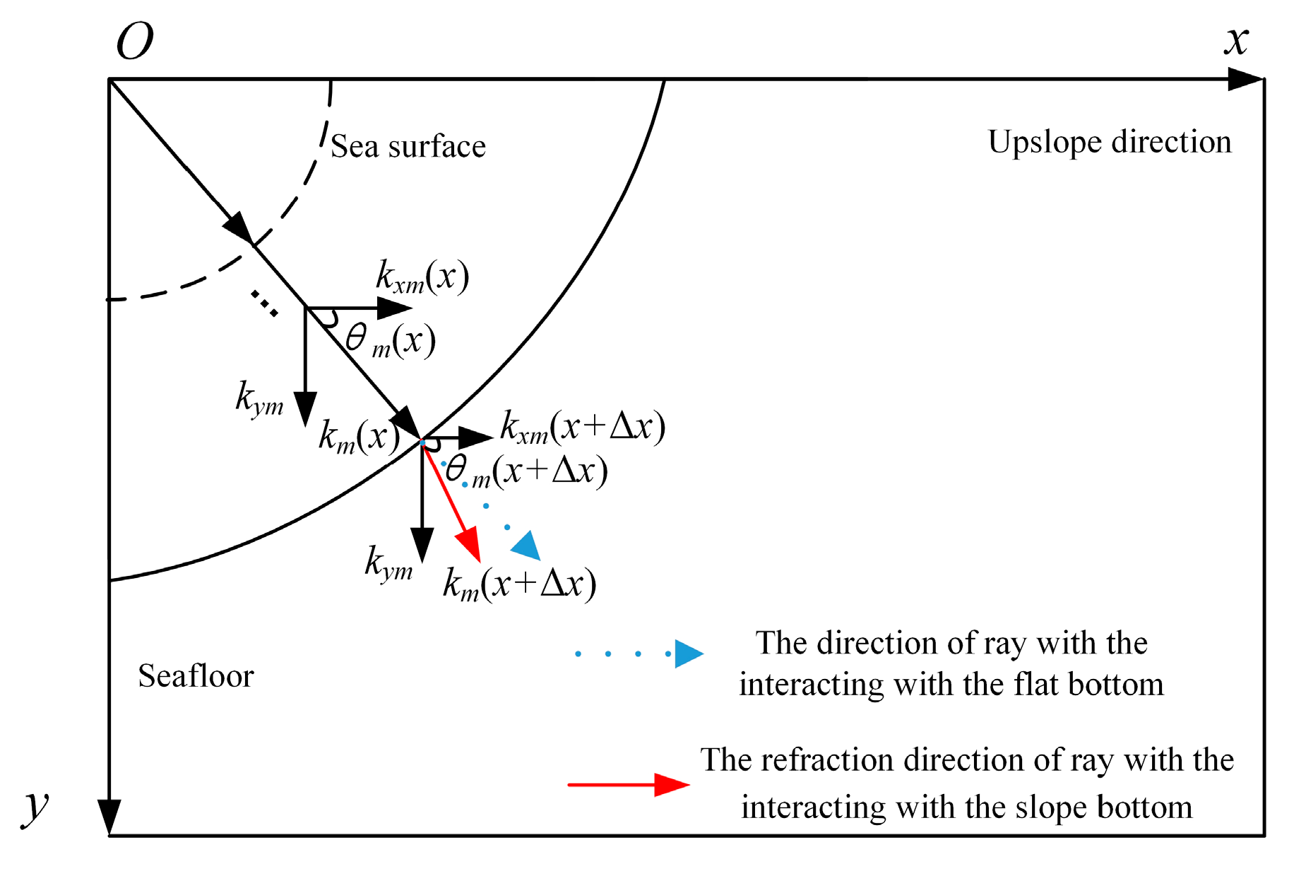
2.2. Horizontal Refraction with the Coupled-Mode Theory

Research shows that an acoustic ray comprises modes with weighted superpositions [32]. According to generalized ray–mode theory, the energy pulse traveling along the ray path is a weighted summation of modes grouped together, with the ray path corresponding to the central mode in the group [33]. The relationship between the ray of the grazing angle $\gamma$ and the $m$th order of the mode is given by

$$\cos \gamma ={\displaystyle \frac{\mathrm{re}(k_m)}{k_s}}$$

(11)

where $k_s=\omega /c_s$, and $c_s$ is the sound speed at the source depth. “re” indicates the real part of the complex number. Notably, the value of angle $\gamma$ depends on the source depth in the non-isovelocity environment.

The horizontal propagation wavenumber $k_m$ is decomposed into the $k_{xm}$ and $k_{ym}$ components in the $x$- and $y$-directions, respectively. Therefore, the horizontal propagation direction ${\theta }_m(x)$ is defined by

$$\tan {\theta }_m(x)=k_{ym}/k_{xm}(x)$$

(12)

where ${\theta }_m(x)$ indicates the angle of the ray with respect to the $x$-axis for the $m$th order of the mode in the horizontal plane.

Figure 2 presents the concept of the horizontal refraction phenomenon. The path of the ray propagation remains the same after the reflection from the sea surface, considering that the sea surface is a horizontal interface with a constant sound speed and density in the horizontal direction. In contrast, the situation changes when the ray interacts with the seabed, revealing a reduction in the value of $k_{xm}(x)$, as the sea depth decreases along the $x$-axis. In addition, the value of $k_{ym}$ remains constant due to the range-independent environment along the $y$-axis. Therefore, the value of ${\theta }_m(x)$ increases with the decrease in $k_{xm}(x)$.

A series of derivations were performed based on the coupled differential equation presented below to investigate the impact of the waveguide environmental change along the $x$-axis on the horizontal propagation wavenumber $k_{xm}(x)$.

According to normal modes theory, the standard form of source pressure $\overline{p}(x,z;k_{ym})$ [34] is expressed as follows:

$$\overline{p}(x,z;k_{ym})={\displaystyle \frac{i}{2}}{\displaystyle \sum _{m=1}^M{\varphi }_m(0,z_s;k_{ym})}{\varphi }_m(x,z;k_{ym}){\displaystyle \frac{\exp (i{k}_{xm}x)}{k_{xm}}}$$

(13)

By comparing Equations (7) and (13), the expression of $u_m(x,k_{ym})$ is obtained as

$$u_m(x,k_{ym})={\displaystyle \frac{i}{2}}{\displaystyle \frac{{\varphi }_m(0,z_s;k_{ym})}{\sqrt{k_{xm}(x)}}}$$

(14)

The square of the $m$th horizontal wavenumber $k_{xm}(x)$ located at $x$ is

$$\sqrt{k_{xm}(x)}={\displaystyle \frac{i}{2}}{\displaystyle \frac{{\varphi }_m(0,z_s;k_{ym})}{u_m(x,k_{ym})}}$$

(15)

According to the first-order finite difference, $k_{xm}(x+\Delta x)$ located at ($x+\Delta x$) is calculated step-to-step as follows:

$$\begin{array}{ll}\sqrt{k_{xm}(x+\Delta x)}& ={\displaystyle \frac{i}{2}}{\displaystyle \frac{1}{u_m\left(x+\Delta x;k_{ym}\right)}}{\varphi }_m\left(0,z_s;k_{ym}\right)\\ & ={\displaystyle \frac{i}{2}}{\displaystyle \frac{1}{u_m\left(x;k_{ym}\right)+\Delta x\left[\partial u_m\left(x;k_{ym}\right)/\partial x\right]}}{\varphi }_m\left(0,z_s;k_{ym}\right)\end{array}$$

(16)

where $\Delta x$ is the distance grid. The separation of the amplitude and phase of the $m$th order of the mode is as follows:

$$u_m\left(x;k_{ym}\right)=u_m(x)\exp \left[i{\displaystyle {\int }_0^x\left(k_{xm}-k_0\right)}ds\right]$$

(17)

The partial derivative of the $m$th mode amplitude in the $x$-direction is

$${\displaystyle \frac{\partial U_m(x)}{\partial x}}=-{\displaystyle \sum _{\begin{array}{c}n=1\\ n\ne m\end{array}}^N{B}_{mn}}{U}_m(x)\exp \left[i{\displaystyle {\int }_0^x\left(k_{xn}-k_{xm}\right)}ds\right]$$

(18)

Substituting Equations (17) and (18) into Equation (16) yields $\sqrt{k_{xm}(x+\Delta x)}$, which is located at ($x+\Delta x$)

$$\begin{array}{ll}\sqrt{k_{xm}(x+\Delta x)}& ={\displaystyle \frac{i}{2}}{\displaystyle \frac{1}{U_m\left(x+\Delta x;k_{ym}\right)}}{\varphi }_m\left(0,z_s;k_{ym}\right)\\ & ={\displaystyle \frac{i}{2}}{\displaystyle \frac{{\varphi }_m\left(0,z_s;k_{ym}\right)\exp \left[i{\displaystyle {\int }_0^{x+\Delta x}\left(k_0-k_{xm}\right)}ds\right]}{U_m(x)\exp \left[i{\displaystyle {\int }_0^x\left(k_{xm}\right)}ds\right]-\Delta x{\displaystyle \sum _{\begin{array}{c}n=1\\ n\ne m\end{array}}^N\left\{B_{mn}(x)U_n(x)\exp \left[i{\displaystyle {\int }_0^x\left(k_{xn}\right)}ds\right]\right\}}}}\end{array}$$

(19)

Notably, the influence of the horizontal variation in environmental parameters on the change in wavenumber $k_{xm}$ is mainly reflected in the denominator part of Equation (19).

To facilitate description, the following is presented for the $m$th mode:

$${\mathsf{\Omega }}_m(x)=U_m(x)\exp \left(i{\displaystyle {\int }_0^x{k}_{m}ds}\right)$$

(20)

The coupling term in Equation (19) can be written as follows:

$${\mathsf{\Psi }}_m(x)={\displaystyle \sum _{\begin{array}{c}n=1\\ n\ne m\end{array}}^N\left[B_{mn}(x)U_n(x)\exp \left(i{\displaystyle {\int }_0^x\left(k_{xn}\right)}ds\right)\right]}$$

(21)

Equation (19) can then be simplified to

$$\sqrt{k_{xm}(x+\Delta x)}={\displaystyle \frac{i}{2}}{\displaystyle \frac{\exp \left[i{\displaystyle {\int }_0^{x+\Delta x}\left(k_0-k_{xm}\right)}ds\right]}{{\mathsf{\Omega }}_m(x)-\Delta x{\mathsf{\Psi }}_m(x)}}{\varphi }_m\left(0,z_s;k_{ym}\right)$$

(22)

Furthermore, the effect of mode coupling on horizontal refraction ${\mathsf{{\rm Y}}}_m(x)$ is written as shown below:

$${\mathsf{{\rm Y}}}_m(x)={\mathsf{\Omega }}_m(x)-\Delta x{\mathsf{\Psi }}_m(x)$$

(23)

The value of $k_{xm}(x+\Delta x)$ increases with $\sqrt{k_{xm}(x+\Delta x)}$. Therefore, the effect of mode coupling due to the horizontal variation in environmental parameters on the changing propagation direction can be analyzed using Equation (22). According to the Equations (12) and (22), for the ray of the $m$th mode, the horizontal refraction angle is positively correlated with the modal amplitude of the $m$th order and negatively correlated with the mode coupling influence of the modal amplitude except for the $m$th order. Assuming that energy conversion does not occur between modes, the value of ${\mathsf{\Psi }}_m(x)$ is zero. Therefore, the horizontal refraction angle under the adiabatic approximation assumption is greater than that when mode coupling is considered.

3. Simulation Results

The environmental parameters used in the simulation are presented herein. The sound profile, sourced from the World Ocean Database [35], is illustrated in Figure 3a. The sound profile is truncated corresponding to shifts in the water column depth. The parameters for the bottom sediment include a speed of 1700 m/s, an absorption coefficient of 0.5 dB/$\lambda$, and a density of 1.5 g/cm³. The water column depth at the source location is 1000 m.

The grazing angle of the source corresponding to the modal order and the eigenfunctions according to the Equation (11) and waveguide environment are depicted in Figure 3b,c, respectively. Notably, in an environment with an incomplete vertical sound speed structure, the grazing angle of the low-order mode is almost equal to zero because the real part of the eigenvalue of these modes is larger than the wavenumber at the source location. Additionally, the value of eigenfunctions at the source depth approaches zero, as shown in Figure 3c.

Figure 4 shows the variation in horizontal refraction angles after a seafloor interaction for different-order modes of the rays. The slope inclination angle is 3°. Notably, a smaller horizontal refraction angle is observed at a smaller horizontal emergence angle. At a relatively large horizontal emergence angle, the component $k_{ym}$ of the horizontal wavenumber $k_m$ along the $y$-axis is also large. In this situation, the variation in component $k_{xm}$ is highly discernible along the $x$-axis, thereby influencing the horizontal refraction angle.

Figure 4 shows an interesting phenomenon. It is well known that the horizontal refraction angle increases with the order of the mode, but the refraction angles are equal in the case of low-order modes at the same source depth. When the grazing angle approaches zero, as depicted in Figure 3b, the horizontal refraction angle remains the same and does not vary with the corresponding modal order. Furthermore, the horizontal refraction angle decreases with the increase in source depth. It can be found that the horizontal refraction is related to the modal order and the source depth, and the modal coupling is caused by the horizontal environment variation.

According to Equation (22), the horizontal refraction angle is influenced by the source depth, the source frequency, and the slope inclination angle. Further analyses of mode coupling effects are presented below.

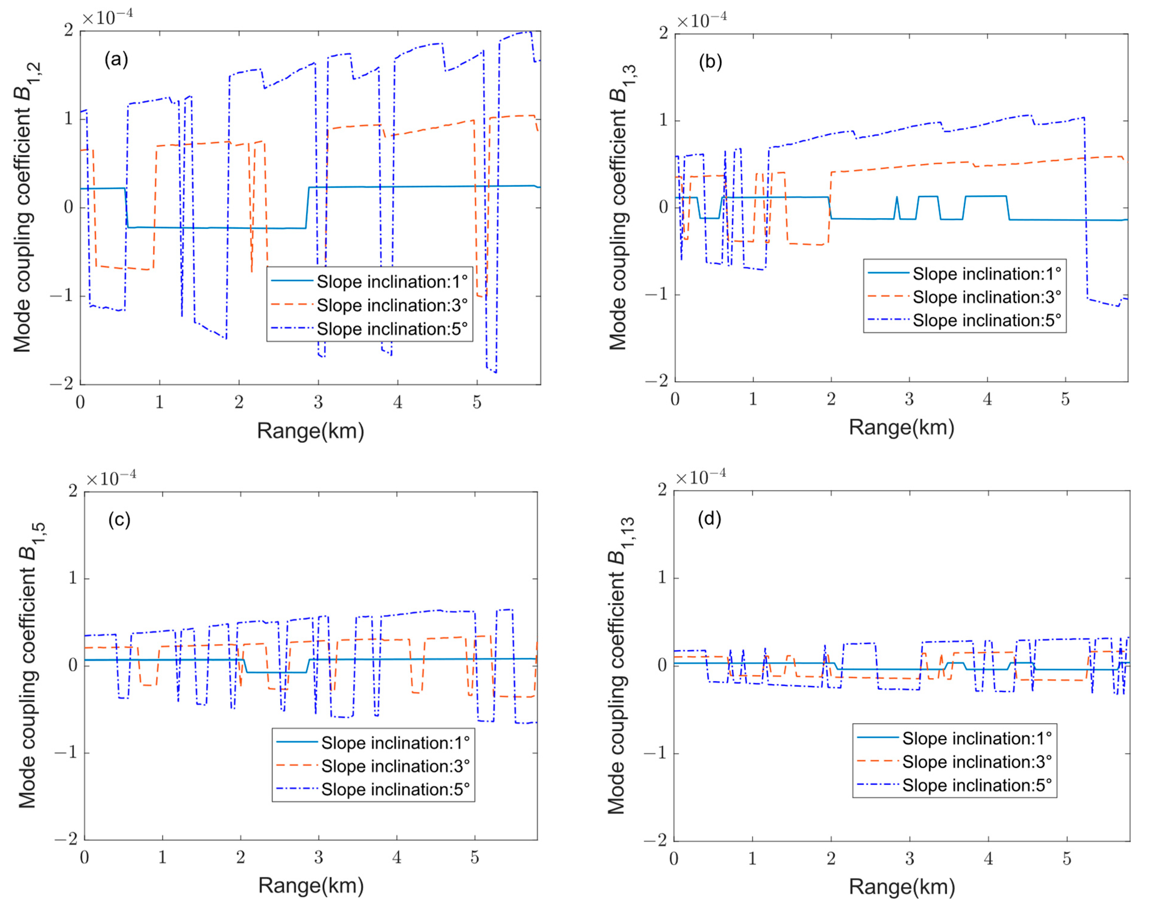
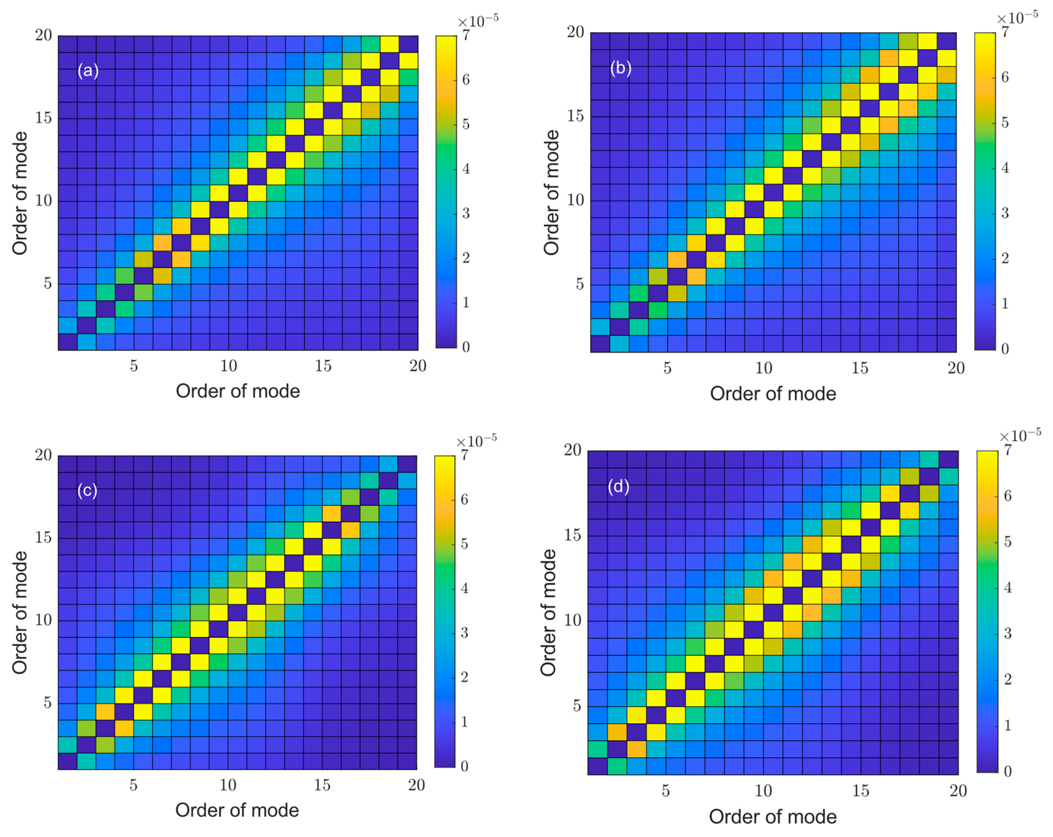
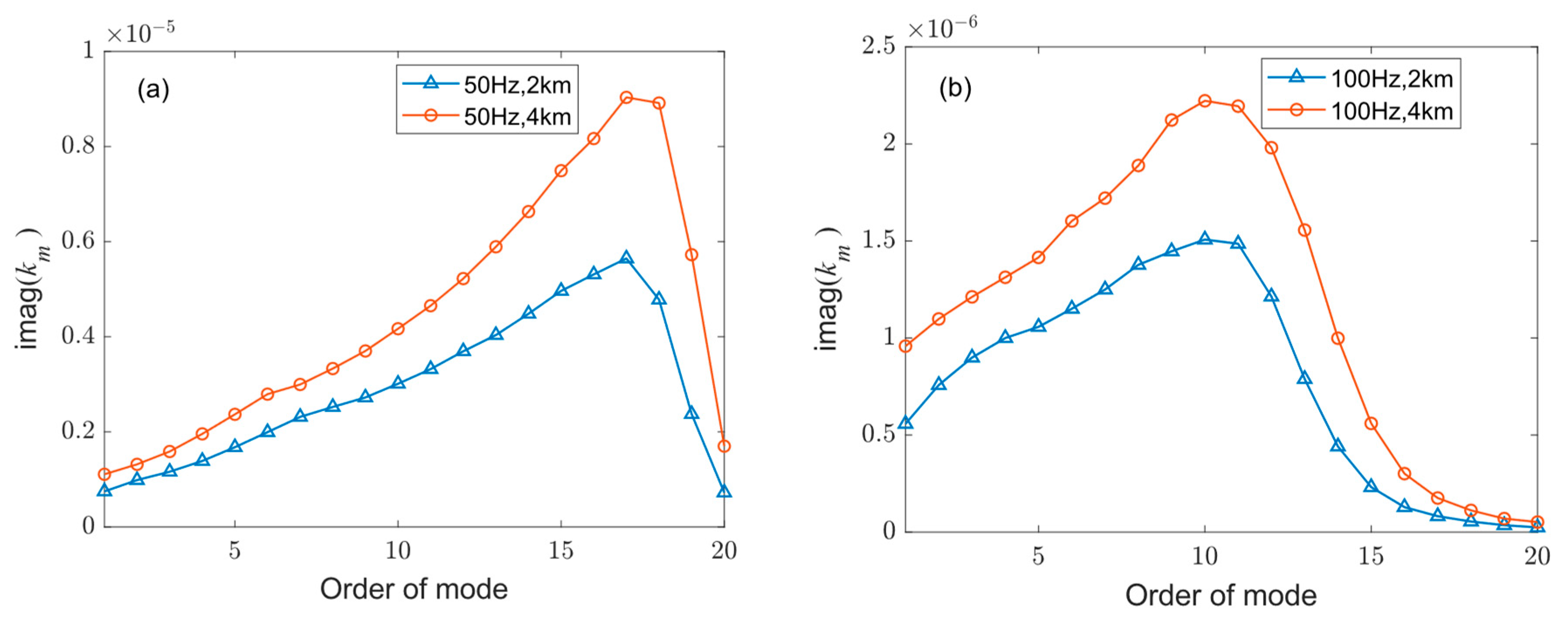
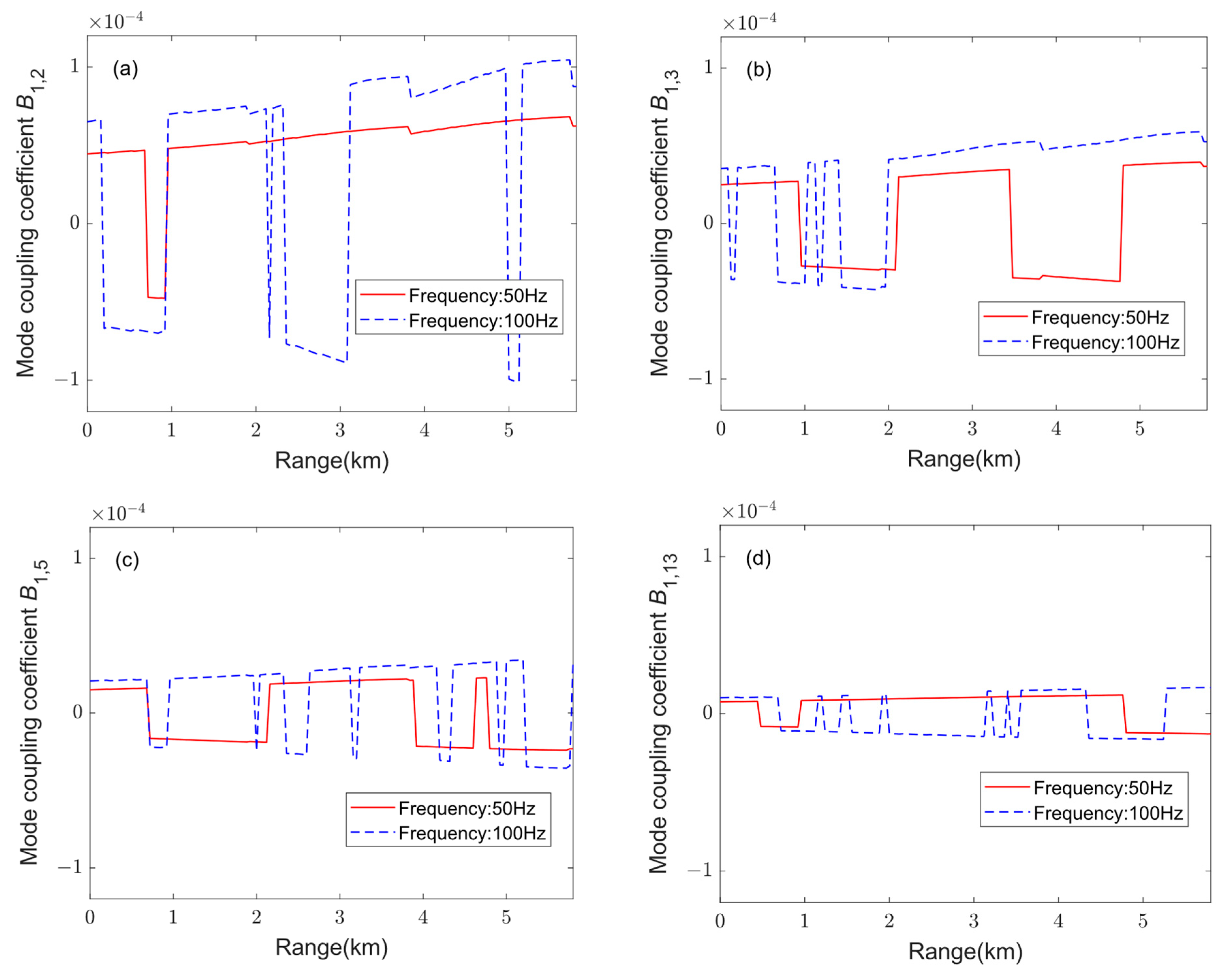
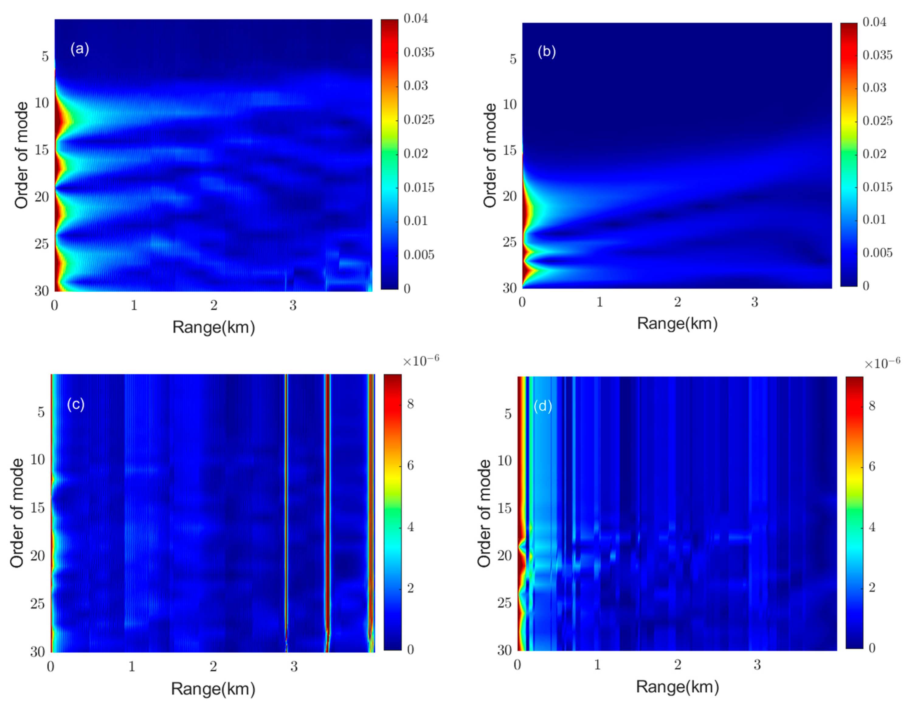
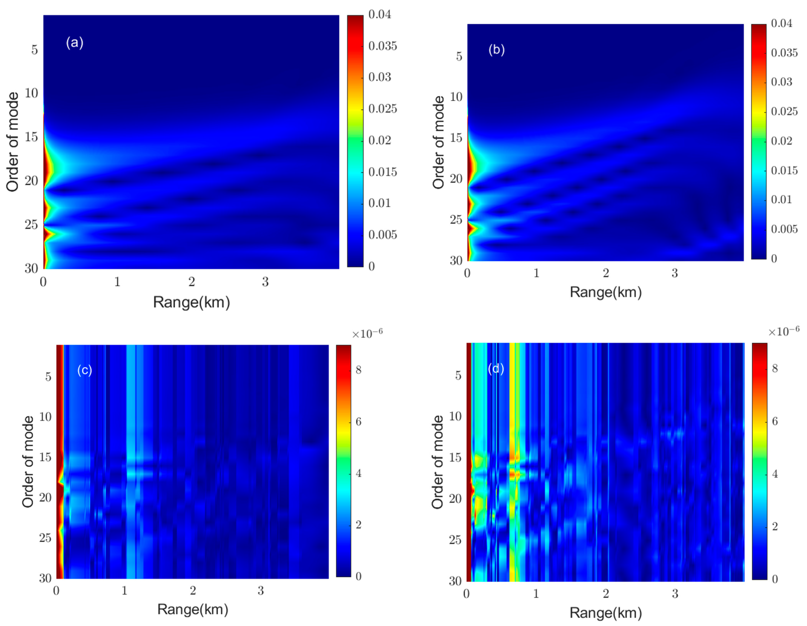
3.1. Mode Coupling Coefficients

The matrix element $B_{mn}$ indicates the energy transduction from the $m$th mode to the $n$th mode. The extent of mode coupling is influenced by the range-dependent environment, particularly the slope inclination angle and the source frequency.

The inter-mode coupling coefficient is shown in Figure 5, representing the inter-mode coupling coefficient at ranges of 0–5.8 km of the 1st order with the 2nd, 3rd, 5th, and 15th orders. The range indicates the distance from the source to the receive location along the $x$-axis. According to normal mode theory, the modal eigenfunctions are calculated in the local waveguide environment. According to Equation (10), the mode coupling coefficient is calculated using the modal eigenfunctions, and the range grid is 0.2 m.

It is found that the amplitude of inter-mode coupling coefficient $B_{1,n}$ decreases as the value of $n$ increases. The energy exchange between adjacent modes evidently occurs with the horizontal variation in the waveguide environment. The oscillation amplitude of the inter-mode coupling coefficient with the same order becomes large as the range increases. Additionally, the growth rate along the range of the amplitude of coefficient $B_{1,n}$ decreases as the value of $n$ increases. However, the oscillation amplitude of coefficient $B_{1,n}$ increases with the slope angle. As the slope inclination angle increases, the structure of the eigenfunctions dramatically changes in the horizontal direction, thereby exacerbating the energy exchange between modes.

Figure 6 shows the mode coupling coefficients as the function of source frequency. The figure reveals that the lower-order modal energy of the low-frequency signal is more stable at the same range, while its higher-order modal energy is more likely to be exchanged with neighboring modal energy. Figure 7 presents the imaginary parts of eigenvalues with 50 and 100 Hz frequencies, thereby explaining this phenomenon. As shown in Figure 7a, at a frequency of 50 Hz, the imaginary part of the eigenvalue of higher-order modes notably increases with the decreasing depth of seawater, thereby more energy is transferred to nearby orders of modes. In contrast, at a frequency of 100 Hz, the imaginary part of the eigenvalue around the 10th-order mode substantially increases, and the corresponding mode coupling coefficient value is large (Figure 7b). Figure 8 shows the variation in the inter-mode coupling coefficient with range at different frequencies. This figure indicates that the oscillation amplitude of the inter-mode coupling coefficient at a higher frequency is greater than that at lower frequency. Furthermore, the inter-mode coupling coefficient $B_{1,n}$ of low-frequency signals is relatively stable.

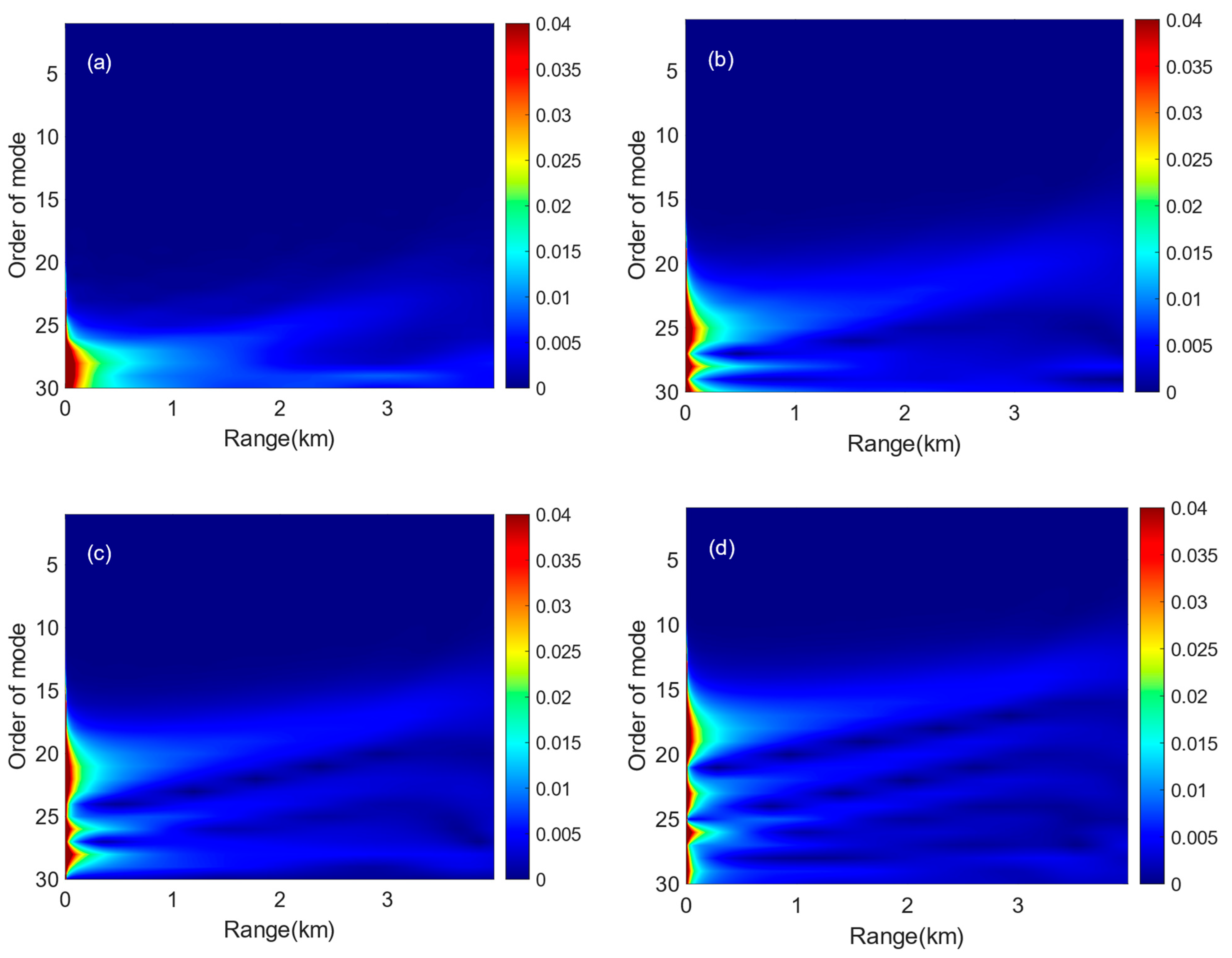
3.2. Effect of Mode Coupling on the Horizontal Refraction

According to Equation (22), the effect of mode coupling on the horizontal propagation wavenumber $k_{xm}$ along the $x$-axis has a relationship with two parts: the modal amplitude ${\mathsf{\Omega }}_m(x)$ and the mode coupling influence except the $m$th order ${\mathsf{\Psi }}_m(x)$. The modal amplitude is excited by the sound source; therefore, the depth and frequency of the source affect mode coupling. Furthermore, the horizontal variation degree of the waveguide environment caused by the slope angle impacts the propagation modal amplitude. The effects of the source depth, frequency, and slope inclination angle on the mode coupling phenomenon are discussed below.

Figure 9 shows the relationship between the source depth and the excited modal amplitude. When the source is close to the surface, the higher orders of primary modes are excited. Conversely, as the source depth increases, the dominant excited modes gradually decrease in order, but the intensity of the excited modes increases, as shown in Figure 9a–d. Figure 9a shows that when the sound source is near the surface, the energy of the excited higher-order modes rapidly attenuates with distance. Additionally, the number of excited orders of the mode increases with the sound source depth. This phenomenon promotes energy propagation over long distances. Furthermore, the decrease in the depth changes the eigenfunction structure, resulting in a highly complex distribution of mode amplitudes along the modal dimension as distance increases. Consequently, the energy tends to shift toward low-order modes, as shown in Figure 9d.

Figure 10 depicts the amplitude of ${\mathsf{\Psi }}_m(x)$, indicating the effect of mode coupling except for the $m$th order. The value of ${\mathsf{\Psi }}_m(x)$ is notably lower than that of ${\mathsf{\Omega }}_m(x)$. For the $m$th mode, the impact of the other orders of modes is modulated by the coupling coefficient matrix, and the influence of those modes on horizontal refraction is considerably smaller than that of the $m$th mode. This finding indicates that the adiabatic assumption can be used when the effect of the modal amplitude on horizontal refraction is small. When the source depth is shallower, fewer dominant modes are excited, resulting in a lower overall influence of the other mode than that at a deeper source depth. With the same frequency and slope inclination angle, the disturbance of ${\mathsf{\Omega }}_m(x)$ demonstrates that the order of the mode is mainly excited by the source. As shown in Figure 10a, the disturbance of stripes is noticeable around the 28th order, corresponding to Figure 9a, and the orders of the mode decrease with the increase in range.

Figure 11 depicts the effect of the frequency on the values of ${\mathsf{\Omega }}_m(x)$ and ${\mathsf{\Psi }}_m(x)$. When the source frequency is low, more dominant modes are excited at the same source depth. Meanwhile, compared to higher-frequency signals, the high-order mode components of low-frequency signals are more substantially affected by distance, as shown in Figure 11a,b. This phenomenon is due to the larger mode coupling amplitude of low-frequency signals in the higher-order parts compared to that of high-frequency signals, thereby resulting in a greater extent of energy exchange. Additionally, a higher frequency results in a greater overall influence of the other modes except for the $m$ th, as shown in Figure 11c,d.

Figure 12 further analyzes the impact of the slope inclination angle on the values of ${\mathsf{\Omega }}_m(x)$ and ${\mathsf{\Psi }}_m(x)$. When the slope inclination angle is steeper, the change in water depth within the same distance grid is substantial, and the modal eigenfunctions are compressed to a greater extent in the depth direction during upward propagation. This phenomenon affects the mode coupling coefficient and modal propagation amplitude. As shown in Figure 12a,b, the stripes become steep as the slope inclination angle increases. Despite the same source depth exciting the same number of modes, with a steeper slope inclination angle, the influence of modes except the $m$th is substantially greater than that at a smaller slope inclination angle, and the resulting interference stripes are highly complex. When the slope inclination angle is large, the degree of mode coupling intensifies, leading to greater energy exchange between modes.

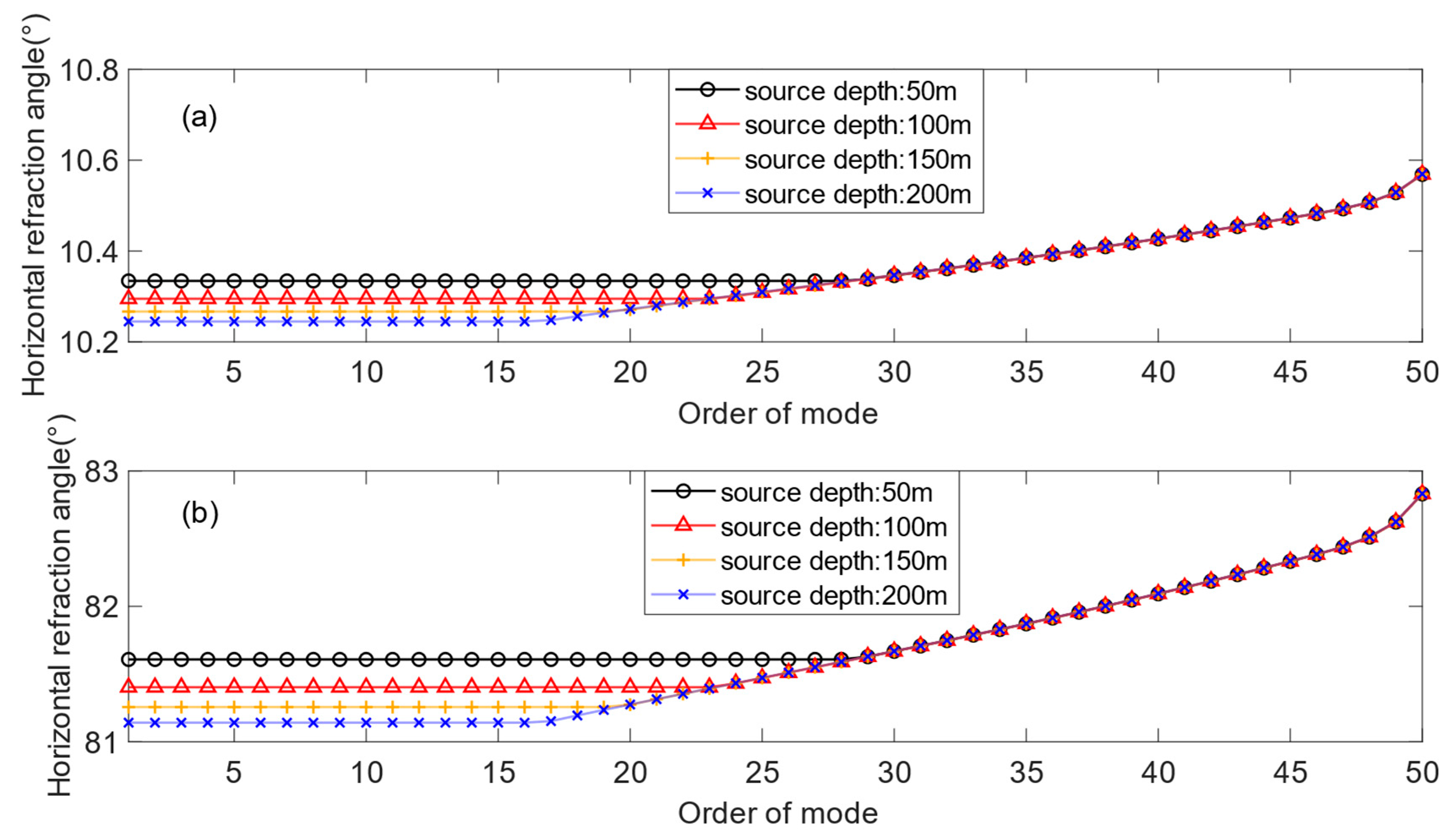
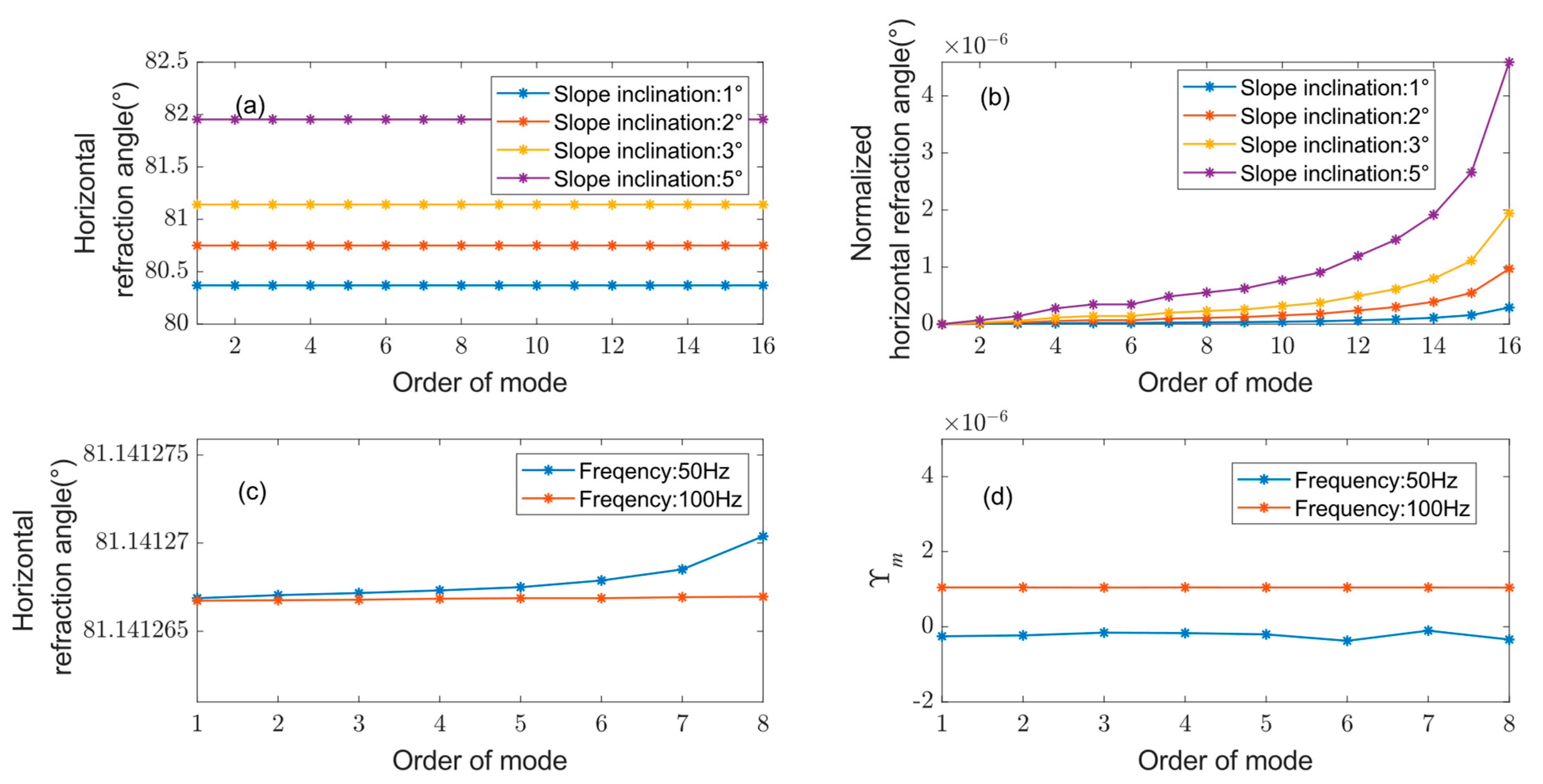
3.3. Horizontal Refraction Angle

The impacts of the frequency, source depth, and slope inclination angle on the mode coupling coefficient, as well as the values of ${\mathsf{\Omega }}_m(x)$ and ${\mathsf{\Psi }}_m(x)$, have been examined above. This section will investigate the horizontal refraction angle patterns under this condition for modal orders where the real part of the horizontal wavenumber $k_m$ is greater than the wavenumber $k_s$ at the source location. This simulation fixes the horizontal emergence angle at 80°, increasing the prominence of the horizontal refraction phenomenon. According to the horizontal emergence angles and grazing angle of the source, the location $x$ where the ray corresponding to the modal orders interacts with the seabed first is calculated based on Snell’s law. The horizontal refraction angle is calculated by the Bellhop3D model. Comparing the influence of ${\mathsf{{\rm Y}}}_m$ and the values of eigenfunctions at the source depth on horizontal refraction, the value of ${\mathsf{\Lambda }}_m$ is written as follows:

$${\mathsf{\Lambda }}_m={\displaystyle \frac{{\mathsf{{\rm Y}}}_m}{{\varphi }_m(0,z_s;k_{ym})}}$$

(24)

Figure 13a shows the horizontal refraction angles of the ray corresponding to the 1st to the 16th order of the mode at different source depths. Notably, a deeper source depth leads to a greater horizontal refraction angle. The value of ${\mathsf{\Lambda }}_m$ is depicted in Figure 13b, which compares the magnitudes of the effects of the values of eigenfunctions and modal coupling. The minimum value of ${\mathsf{\Lambda }}_m$ in Figure 13b is 0.0531, and some values of ${\mathsf{\Lambda }}_m$ are greater than 1 at certain orders of the mode. It can be found that the values of ${\mathsf{{\rm Y}}}_m$ and modal eigenfunctions ${\varphi }_m(0,z_s;k_{ym})$ at the source depth are of similar magnitudes. This finding indicates that the mode coupling effect exerts a considerable influence on the horizontal refraction at these orders of mode.

At different source depths, the ray corresponding to the same order of the mode has a different propagation distance after the first interaction with the seafloor. Figure 13c depicts the value of parameter ${\mathsf{\Psi }}_m(x)$, showing the effect of mode coupling except for the $m$th order on horizontal refraction. A deeper source depth results in a greater influence of mode coupling of the other orders. Considering this phenomenon, according to Equations (13) and (21), a shallower source depth leads to a larger horizontal refraction angle. The effect of the modal order on horizontal refraction was also analyzed with the same source depth by normalizing the horizontal refraction angle of the first-order mode. The horizontal refraction angle increases with the order. However, the increment of the angle is extremely minute and can be ignored in practice.

Further analysis of the influence of the slope inclination angle and frequency on the horizontal refraction angle was conducted, as described below. In the simulation, the source depth is 200 m, and the frequency is 100 Hz. The horizontal refraction angle and normalized horizontal refraction angle of the ray corresponding to the modal order at different slope inclination angles are shown in Figure 14a,b, respectively. Notably, the horizontal refraction angle of the ray corresponding to the low-order mode is nearly the same for the identical slope inclination angle. The increment is still extremely minute, even though the refraction angle increases with the modal order.

The horizontal refraction angles of the ray corresponding to different modal orders at different frequencies are depicted in Figure 14c. However, the difference in horizontal refraction angles between 50 and 100 Hz frequencies is highly negligible. In contrast to the frequency of 100 Hz, the horizontal refraction angle at a 50 Hz frequency ascends more rapidly as the order of the mode increases. The values of ${\mathsf{{\rm Y}}}_m$ that characterize the influence of other-order modes are shown in Figure 14d. It can be found that the values of ${\mathsf{{\rm Y}}}_m$ at 50 Hz are lower than those at 100 Hz. According to Equations (13) and (21), the smaller influence of modes except for the $m$th leads to greater angles of horizontal refraction. Hence, a lower frequency results in a greater horizontal refraction angle.

4. Conclusions

In the sloping sea area with an incomplete vertical sound speed structure, rays corresponding to the low-order normal mode exhibit similar horizontal refraction angles at low frequencies. To interpret this phenomenon, based on the model coupling theory, this paper investigates the energy transformation process between the modes after the ray interacts with the seabed and analyzes the variations of horizontal wavenumber and propagation direction. Furthermore, the impact of source depth, slope inclination, and frequency on the propagation pattern is analyzed.

The results indicate that the horizontal refraction phenomenon is related to the source depth and the modal order of the ray. In the event of an incomplete vertical sound speed profile, the influence of the modal order on the horizontal refraction angle can be estimated by comparing the real part of the horizontal propagation wavenumber $k_m$ with the wavenumber $k_s$ at the source location.

First, if re$(k_m)$ is less than $k_s$, then the horizontal refraction angle predominantly depends on the order of the mode. The horizontal refraction angle of the ray corresponding to the same modal order remains unchanged despite variations in source depth. Second, if re$(k_m)$ is larger than $k_s$, then the horizontal refraction angle is mainly influenced by the source depth. The horizontal refraction angle decreases as the depth of the sound source increases. Notably, the ray with the same source depth has the same horizontal refraction angle, as long as re$(k_m)$ is larger than $k_s$. This condition is due to the extremely small eigenfunction value at the source depth of the low-order mode, thereby enhancing the mode coupling effect. The mode coupling is intimately associated with the mode excited by the sound source. Therefore, the source depth exerts a substantial influence on the horizontal refraction.

The research presented in this paper revealed several potential future applications. In transition-zone waveguide environments, the horizontal refraction angle of the lower mode is correlated with the source depth, which can be leveraged for source depth estimation. Additionally, the frequency exerts less of an impact on the lower modes, making it valuable for processing horizontally refracted signals using wideband array processing methods.

References

1. Weston, D.E. Horizontal refraction in a three-dimensional medium of variable stratification. J. Acoust. Soc. Am. 1961, 78, 46. [Google Scholar] [CrossRef]
2. Harrison, C.H. Three-dimensional ray paths in basins, troughs, and near seamounts by use of ray invariants. J. Acoust. Soc. Am. 1977, 62, 1382–1388. [Google Scholar] [CrossRef]
3. Harrison, C.H. Acoustic shadow zones in the horizontal plane. J. Acoust. Soc. Am. 1979, 65, 56–61. [Google Scholar] [CrossRef]
4. Buckingham, M.J. Theory of acoustic propagation around a conical seamount. J. Acoust. Soc. Am. 1986, 80, 265–277. [Google Scholar] [CrossRef]
5. Luo, W.; Schmidt, H. Three-dimensional propagation and scattering around a conical seamount. J. Acoust. Soc. Am. 2009, 125, 52–65. [Google Scholar] [CrossRef]
6. Arnold, J.M.; Felson, L.B. Rigorous Theory of Horizontal Refraction in a Wedge Shaped Ocean. In Progress in Underwater Acoustics; Merklinger, H.M., Ed.; Springer: Boston, MA, USA, 1987; pp. 549–556. [Google Scholar] [CrossRef]
7. Jensen, F.B.; Kuperman, W.A. Sound propagation in a wedge-shaped ocean with a penetrable bottom. J. Acoust. Soc. Am. 1980, 67, 1564–1566. [Google Scholar] [CrossRef]
8. Westwood, E.K. Broadband modeling of the three-dimensional penetrable wedge. J. Acoust. Soc. Am. 1992, 92, 2212–2222. [Google Scholar] [CrossRef]
9. Deane, G.B.; Buckingham, M.J. An analysis of the three-dimensional sound field in a penetrable wedge with a stratified fluid or elastic basement. J. Acoust. Soc. Am. 1993, 93, 1319–1328. [Google Scholar] [CrossRef]
10. Tang, J.; Petrov, P.S.; Piao, S.; Kozitskiy, S.B. On the Method of Source Images for the Wedge Problem Solution in Ocean Acoustics: Some Corrections and Appendices. Acoust. Phys. 2018, 64, 225–236. [Google Scholar] [CrossRef]
11. Weinberg, H.; Burridge, R. Horizontal ray theory for ocean acoustics. J. Acoust. Soc. Am. 1974, 55, 63–79. [Google Scholar] [CrossRef]
12. Heaney, K.D.; Campbell, R.L.; Murray, J.J. Comparison of hybrid three-dimensional modeling with measurements on the continental shelf. J. Acoust. Soc. Am. 2012, 131, 1680–1688. [Google Scholar] [CrossRef] [PubMed]
13. Lin, Y.; Uffelen, L.J.V.; Miller, J.H.; Potty, G.R.; Vigness-Raposa, K.J. Horizontal refraction and diffraction of underwater sound around an island. J. Acoust. Soc. Am. 2022, 151, 1684–1694. [Google Scholar] [CrossRef]
14. McDonald, B.E.; Collins, M.D.; Kuperman, W.A.; Heaney, K.D. Comparison of data and model predictions for Heard Island acoustic transmissions. J. Acoust. Soc. Am. 1994, 96, 2357–2370. [Google Scholar] [CrossRef]
15. Dong, Y.; Piao, S.; Gong, L. Effect of three-dimensional seamount topography on very low frequency sound field in deep water. J. Harbin Eng. Univ. 2020, 41, 1464–1470. [Google Scholar] [CrossRef]
16. Heaney, K.D.; Campbell, R.L. Three-dimensional parabolic equation modeling of mesoscale eddy deflection. J. Acoust. Soc. Am. 2016, 139, 918–926. [Google Scholar] [CrossRef]
17. Pinson, S.; Quilfen, V.; Courtois, F.L.; Real, G.; Fattaccioli, D. Shallow-water waveguide acoustic analysis in a fluctuating environment. J. Acoust. Soc. Am. 2022, 152, 1252–1262. [Google Scholar] [CrossRef]
18. Grigor’ev, V.A.; Petnikov, V.G.; Roslyakov, A.G.; Terekhina, Y.E. Sound Propagation in Shallow Water with an Inhomogeneous GAS-Saturated Bottom. Acoust. Phys. 2018, 64, 331–346. [Google Scholar] [CrossRef]
19. Lunkov, A.; Sidorov, D.; Petnikov, V. Horizontal Refraction of Acoustic Waves in Shallow-Water Waveguides Due to an Inhomogeneous Bottom Structure. J. Mar. Sci. Eng. 2021, 9, 1269. [Google Scholar] [CrossRef]
20. Petnikov, V.G.; Grigorev, V.A.; Lunkov, A.A.; Sidorov, D.D. Modeling underwater sound propagation in an arctic shelf region with an inhomogeneous bottom. J. Acoust. Soc. Am. 2022, 151, 2297–2309. [Google Scholar] [CrossRef]
21. Godin, O.A. Manifestations of the weak shear rigidity of marine sediments in amplitudes and travel times of acoustic normal modes and lateral waves. J. Acoust. Soc. Am. 2023, 154 (Suppl. 4), A165. [Google Scholar] [CrossRef]
22. Katsnel’son, B.G.; Malykhin, A.Y. Space-time sound field interference in the horizontal plane in a coastal slope region. Acoust. Phys. 2012, 58, 301–307. [Google Scholar] [CrossRef]
23. Ballard, M.S.; Lin, Y.; Lynch, J.F. Horizontal refraction of propagating sound due to seafloor scours over a range-dependent layered bottom on the New Jersey shelf. J. Acoust. Soc. Am. 2012, 131, 2587–2598. [Google Scholar] [CrossRef] [PubMed]
24. Chaple, R.P.B. Refraction and diffraction of water waves using finite elements with a DNL boundary condition. Ocean. Eng. 2013, 63, 77–89. [Google Scholar] [CrossRef]
25. Mignerey, P.C. Environmentally adaptive wedge modes. J. Acoust. Soc. Am. 2000, 107, 1943–1952. [Google Scholar] [CrossRef]
26. Joe, K.H. Forward Sound Propagation Around Seamounts: Application of Acoustic Models to the Kermit-Roosevelt and Elvis Seamounts. Ph.D. Thesis, Massachusetts Institute of Technology, Cambridge, MA, USA, 2009. Available online: http://hdl.handle.net/1721.1/49764 (accessed on 10 November 2024).
27. Luo, W.; Henrik, S. A Spectral Coupled-Mode Formulation for Sound Propagation around Axisymmetric Seamounts. Chin. Phys. Lett. 2010, 27, 094304. [Google Scholar] [CrossRef]
28. Tang, J. Modelling of Sound Propagation in Wedge-Like Oceans with Elastic Bottom and Analyzing of Horizontal Refraction Effects on Vector Fields. Ph.D. Thesis, Harbin Engineering University, Harbin, China, 2019. [Google Scholar]
29. Luo, W.; Zhang, R.; Schmidt, H. Three-dimensional mode coupling around a seamount. Sci. China Phys. Mech. Astron. 2011, 54, 1561. [Google Scholar] [CrossRef]
30. Mo, Y.; Piao, S.; Zhang, H.; Li, L. Mode coupling and energy transfer in a range-dependent waveguide. Acta Phys. Sin. 2014, 63, 214302. [Google Scholar] [CrossRef]
31. Heaney, K.D.; Murray, J.J. Measurements of three-dimensional propagation in a continental shelf environment. J. Acoust. Soc. Am. 2009, 125, 1394–1402. [Google Scholar] [CrossRef]
32. Wang, D.; Shang, E. Hydroacoustics, 2nd ed.; Science Press: Beijing, China, 2006; pp. 92–98. [Google Scholar]
33. Tindle, C.T.; Guthrie, K.M. Rays as interfering modes in underwater acoustics. J. Sound Vib. 1974, 34, 291–295. [Google Scholar] [CrossRef]
34. Jensen, F.B.; Kuperman, W.A.; Porter, M.B.; Schmidt, H. Computational Ocean Acoustics, 2nd ed.; Springer: New York, NY, USA, 2011; Chapter 5; p. 342. [Google Scholar]
35. World Ocean Sound Speed Database. Available online: https://climatedataguide.ucar.edu/climate-data/world-ocean-atlas-woa09 (accessed on 21 September 2023).
Figure 1. The horizontal refraction scene. (a) Schematic of the ocean waveguide with a wedge bottom. α 0 denotes the slope inclination angle. The speed in the water column c 1 is a function of depth. (b) The horizontal refraction angle.
Jmse 13 00217 g001
Figure 2. An illustration of the horizontal propagation direction of a single ray after individual reactions to the sea surface and seafloor.
Jmse 13 00217 g002
Figure 3. (a) The sound speed profile. The data were adapted from the World Ocean Atlas database [35] (the acoustic profile remains unchanged with range, except that the depth is consistent with the sea depth); (b) the grazing angle corresponding to the order of the mode; (c) modal eigenfunctions. The red circles indicate sound depths of 50, 100, 150, and 200 m from top to bottom.
Jmse 13 00217 g003
Figure 4. The horizontal refraction angle of the ray corresponding to the modal order with a slope inclination angle of 3° after an interaction with the seabed at horizontal emergence angles of (a) 10° and (b) 80°.
Jmse 13 00217 g004
Figure 5. Inter-mode coupling coefficient B 1 , n at ranges of 0–5.8 km of different slope inclination angles. The frequency is 100 Hz. The distance grid for calculating coupling coefficients is 0.2 m. (a) Mode 1 with 2, (b) mode 1 with 3, (c) mode 1 with 5, and (d) mode 1 with 13.
Jmse 13 00217 g005
Figure 6. Mode coupling coefficients with a slope inclination of 3° for the following conditions: (a) the frequency is 50 Hz, and the range is 2 km; (b) the frequency is 50 Hz, and the range is 4 km; (c) the frequency is 100 Hz, and the range is 2 km; and (d) the frequency is 100 Hz, and the range is 4 km.
Jmse 13 00217 g006
Figure 7. Imaginary parts of eigenvalues of the first 20 modes at the ranges of 2 and 4 km at a frequency of (a) 50 Hz and (b) 100 Hz.
Jmse 13 00217 g007
Figure 8. Inter-mode coupling coefficient B 1 , n at ranges of 0–5.8 km for different frequencies with a slope inclination of 3°. (a) Mode 1 with 2; (b) mode 1 with 3; (c) mode 1 with 5; (d) mode 1 with 13.
Jmse 13 00217 g008
Figure 9. The amplitude of the value Ω m ( x ) within ranges of 0–4 km of different source depths at a frequency of 100 Hz with a slope inclination of 3°: (a) source depth is 50 m, (b) source depth is 100 m, (c) source depth is 150 m, and (d) source depth is 200 m.
Jmse 13 00217 g009
Figure 10. The absolute value of Ψ m ( x ) within ranges of 0–4 km at a frequency of 100 Hz with a slope inclination angle of 3° at source depths of (a) 50 m, (b) 100 m, (c) 150 m, and (d) 200 m. The white curves represent the dominant excited modes of different source depths.
Jmse 13 00217 g010
Figure 11. Values of mode coupling within ranges of 0–4 km of different frequencies with a source depth of 150 m and a slope inclination angle of 3°. (a) The amplitude of Ω m ( x ) at a frequency of 50 Hz. (b) The amplitude of Ω m ( x ) at a frequency of 100 Hz. (c) The amplitude of Ψ m ( x ) at a frequency of 50 Hz. (d) The amplitude of Ψ m ( x ) at a frequency of 100 Hz.
Jmse 13 00217 g011
Figure 12. Values of mode coupling within ranges of 0–4 km of different frequencies at a source depth of 200 m and a frequency of 100 Hz. (a) The amplitude of Ω m ( x ) with a slope inclination angle of 3°. (b) The amplitude of Ω m ( x ) with a slope inclination angle of 5°. (c) The amplitude of Ψ m ( x ) with a slope inclination angle of 3°. (d) The amplitude of Ψ m ( x ) with a slope inclination angle of 5°.
Jmse 13 00217 g012
Figure 13. Analysis of the effect of the source depth on the horizontal refraction angle with a slope inclination angle of 3° and a frequency of 100 Hz. (a) The horizontal refraction angle at different source depths; (b) the amplitude of Λ m ; (c) the amplitude of Ψ m ( x ) ; (d) the normalization of the horizontal refraction angle.
Jmse 13 00217 g013
Figure 14. Analysis of the effect of the slope inclination angle and the frequency on the horizontal refraction angle. (a) The horizontal refraction angle with different slope inclination angles with a source depth of 200 m and a frequency of 100 Hz. (b) The normalization of the horizontal refraction angle with a source depth of 200 m and a frequency of 100 Hz. (c) The horizontal refraction angle at different frequencies with a source depth of 200 m and a slope inclination angle of 3°. (d) The amplitude of Λ m with a source depth of 200 m and a slope inclination angle of 3°.
Jmse 13 00217 g014
Disclaimer/Publisher’s Note: The statements, opinions and data contained in all publications are solely those of the individual author(s) and contributor(s) and not of MDPI and/or the editor(s). MDPI and/or the editor(s) disclaim responsibility for any injury to people or property resulting from any ideas, methods, instructions or products referred to in the content.