Abstract
This study investigates the potential of hyperbolic paraboloid (hypar) shapes for enhancing wave attenuation and structural efficiency in Free-Surface Breakwaters (FSBW). A decoupled approach combining Smoothed Particle Hydrodynamics (SPH) and Finite Element Method (FEM) is employed to analyze hypar-faced FSBW performance across varying hypar warping values and wave characteristics. SPH simulations, validated through experiments, determine wave attenuation performance and extract pressure values for subsequent FEM analysis. Results indicate that hypar-faced FSBW produces increased wave attenuation compared to traditional flat-faced designs, particularly for shorter wave periods and smaller drafts. Furthermore, hypar surfaces exhibit up to three times lower principal stresses under wave loading compared to the flat counterpart, potentially allowing for thinner surfaces. The study also shows that peak-load static stress values provide a reasonable approximation for preliminary design, with less than 6% average difference compared to dynamic analysis results. In summary, this research presents hypar-faced FSBW as a promising alternative in coastal defense strategies, offering effective wave attenuation and structural efficiency in the context of rising sea levels and increasing storm intensities.
1. Introduction
The Intergovernmental Panel on Climate Change (IPCC) has reported a strong indication of the rise in sea levels, attributed to the warming of sea temperatures resulting from global warming [1]. This rise in sea levels, coupled with a projected increase in the intensity of tropical storms [2], underscores the critical need for enhanced coastal resilience, especially in densely populated coastal regions [3]. Traditional coastal defense systems, specifically gravity-type bottom-standing breakwaters, while effective in wave attenuation, may present several drawbacks, such as requiring significant material use, disrupting marine habitats, and altering sediment transport. These drawbacks can potentially lead to erosion and other ecological impacts, and can be costly to build and maintain in deeper waters [4,5,6]. For these reasons, Free-Surface Breakwaters (FSBW) offer a promising alternative to traditional gravity-type breakwaters [4].
FSBW, also known as open breakwaters, are barriers positioned near the water surface, where the wave energy flux is dominant [4]. FBSW can be mounted on a series of piles or jacket structures, or they may be maintained in a floating state using mooring cables [4]. FBSW are designed to attenuate the height of incoming waves predominantly through reflection and energy dissipation, proving most effective in environments exposed to wave periods of up to 5 s [7]. Among the various types of FSBW, the box-type breakwater constructed from reinforced concrete (RC) is the most common due to its simple design [4,8]. There has been increasing interest in parametric optimization for Free-Surface Breakwaters (FSBW) designs, particularly in exploring various shapes and configurations such as U- and T-shapes or quadrant front faces [5,7,9,10,11,12,13], as well as alternative approaches like fluid-filled membranes [14], primarily to improve wave attenuation performance, with fewer studies also discussing structural performance [8,15,16]. This presents an opportunity to explore new FSBW forms that are potentially efficient in both wave attenuation and structural performance. One such form is the hyperbolic paraboloid (hypar) surface.
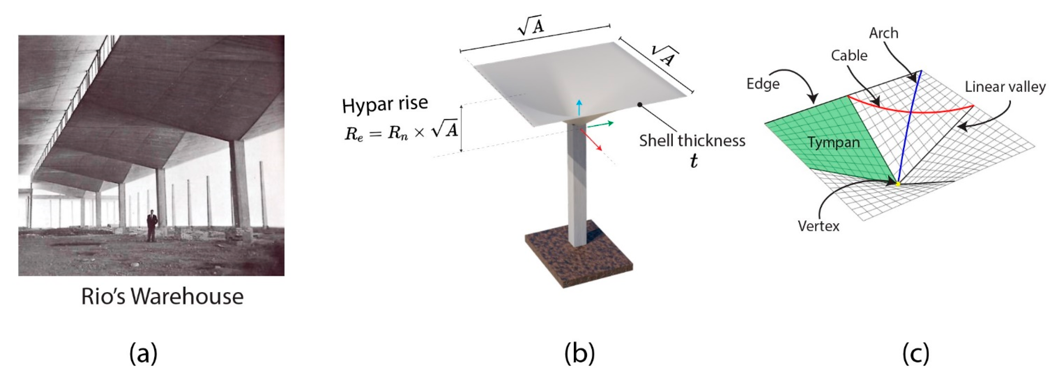
Hypars are doubly curved shell structures featuring “arches” that carry compressive forces from the corners to the vertex, balanced by “cables” in tension in the opposite direction (Figure 1), thereby contributing to structural efficiency [17,18]. Additionally, the straight-line generators of the hypars in two directions, as shown in Figure 1, aid in construction by facilitating the use of linear elements in both formwork and reinforcing steel [19].
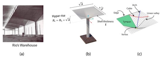
Figure 1.
Four-edged hypar umbrella. (a) A real-world example of this type of umbrella in Mexico, image courtesy of Princeton University Library’s Department of Special Collections. (b) Rendering defining the geometric parameters. (c) Hypar shell showing straight-line generators.
The most notable designer of hypar-formed roofs in the 20th century is Felix Candela [20], who designed hundreds of hypar-roofed structures, mostly in Mexico [20]. In the last two decades, research interest in hypar surfaces within architecture and engineering extended to the near coast. For example, Wang et al. [21,22,23] have proposed using hypar umbrellas as deployable flood barriers that function as a canopy during normal weather, without restricting beach access, and deploy into impermeable barriers during severe weather conditions. In one study, Wang et al. [23] investigated the structural behavior of these umbrellas under hydrostatic inundation, considering factors such as hypar warping (), inundation height, and lateral column stiffness. Smoothed particle hydrodynamics (SPH) were employed to calculate fluid forces, which were then applied to a structural model analyzed using finite element method (FEM) to evaluate stresses and deformations in the shell. The results demonstrated that employing hypar geometry significantly reduces bending and shear stress compared to flat plates, underscoring the structural benefits of hypar shapes. Furthermore, the research investigated the effect of longitudinal asymmetry of hypars on structural behavior, indicating that increased asymmetry increases the demands on the shell and its supporting structures [23]. In a subsequent study, Wang et al. [23] validated a decoupled SPH-FEM model through a series of dam-break experiments on 140 × 140 mm 3D-printed hypar umbrella specimens and by comparing the numerical results with Goda’s formula for wave pressure on a flat plate. The study confirmed the effectiveness of the SPH-FEM model in capturing the complex hydrodynamic behavior of the hypar umbrellas. Validated models were then used to assess the feasibility of Kinetic Umbrellas as deployable flood barriers during a realistic hurricane scenario based on Hurricane Sandy (2012) [23].
Furthermore, Wu et al. [24] revealed that the hydrodynamic wave pressure on the hypar follows a bilinear-like shape along the height and increases gradually from the edge to the longitudinal spine. The same study found that the maximum displacement and tensile forces of the hypar shell were significantly underestimated by Goda’s formula, underscoring the importance of dynamic analyses in accurately assessing the structural response of hypar umbrellas. For other critical demands, such as maximum shell moment and shear force, the difference between static and dynamic analyses was less than 20% [24].
Additionally, ElDarwich et al. [25] investigated the wave attenuation performance of hypar surfaces as faces of box-type FSBW, as illustrated in Figure 2, under regular waves with high-steepness. The study employed a 2D numerical wave flume using SPH to simulate the interaction of regular waves with a FBSW. The results demonstrated that hypar-faced FSBW, due to their curvature, can reduce wave transmission more effectively than their flat-faced counterpart [25]. This finding suggests that hypar geometry can be a viable alternative for improving the wave attenuation performance of FSBW [25].

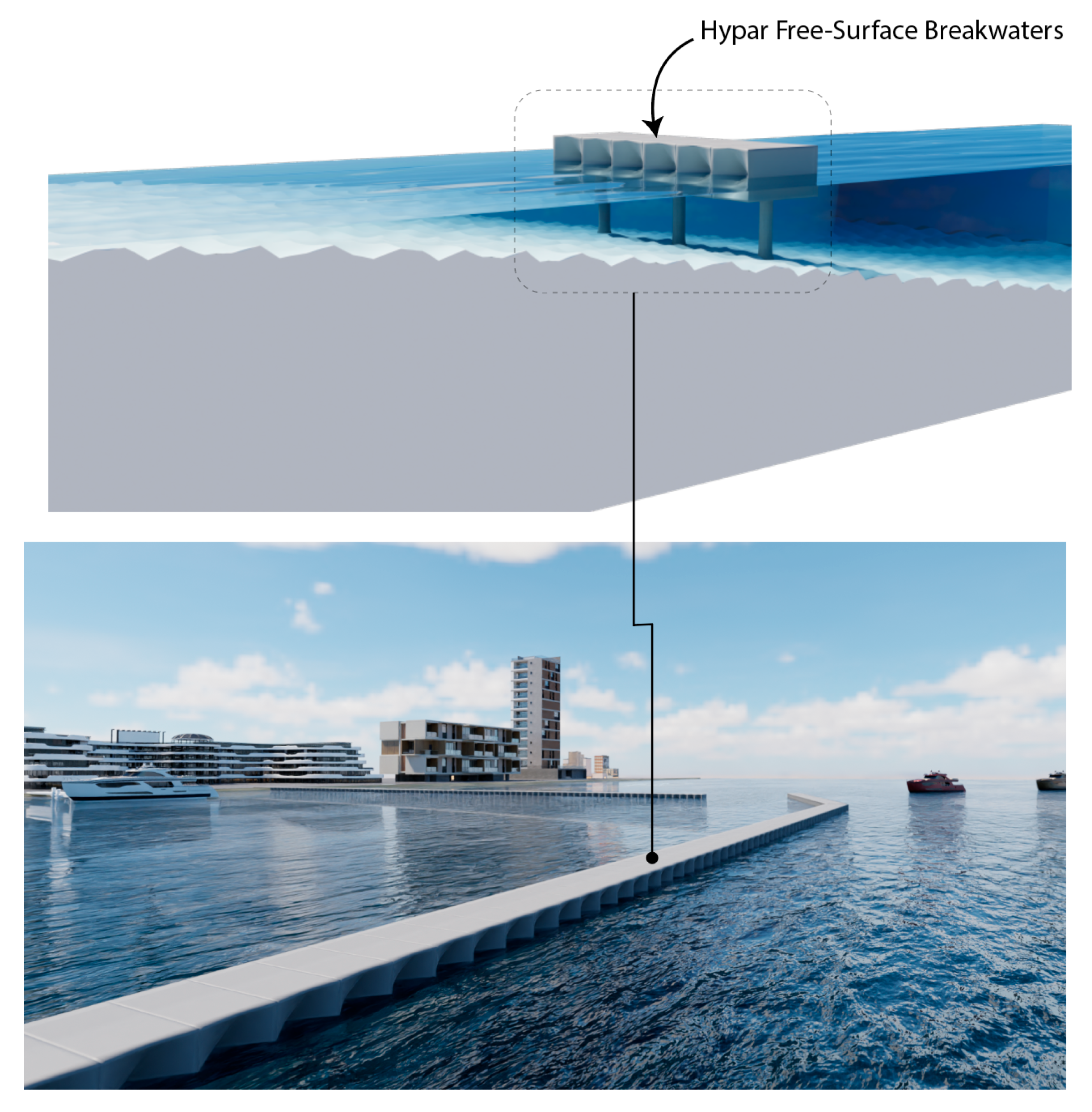
Figure 2.
Artistic rendering of a hypar FSBW, showcasing a protected region (such as a harbor or marina) on the left and the seaside on the right.
Previous work on hypar-faced FSBW has been limited to 2D numerical simulations, focusing solely on wave attenuation performance without addressing structural response. The current study builds on the promising results of the preliminary study. The novel objective of this paper is thus to present a comprehensive 3D analysis of fixed hypar-faced FSBW, evaluating both their hydrodynamic performance and structural response across a wide range of wave periods and drafts, utilizing both SPH numerical simulations and experimental validation.
2. Methodology
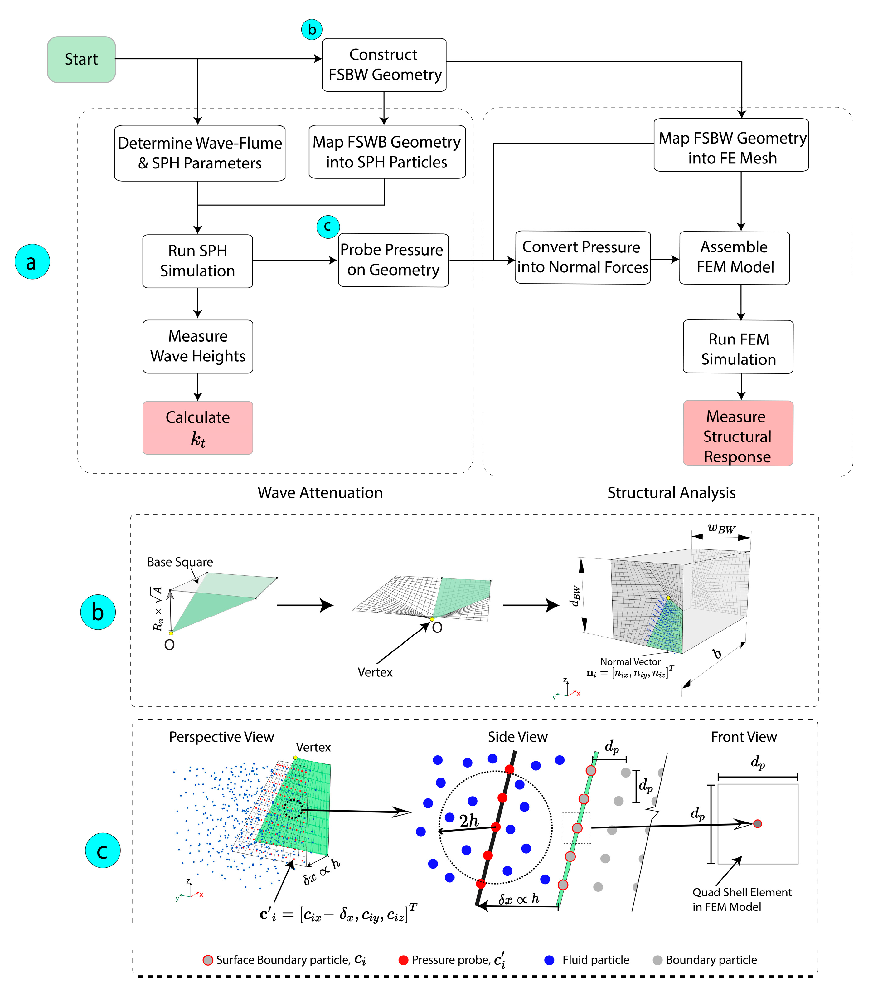
This study employs a decoupled SPH-FEM methodology, previously applied to hypar structures in coastal engineering [21,23,24], as illustrated in Figure 3. In most coastal engineering applications, it is reasonable to model structures as stationary objects in numerical simulations of wave-structure interactions [26]. The process begins with parametrically generating the geometry in Rhino Grasshopper [27], followed by SPH analysis using DualSPHysics [28], a popular open-source software for SPH simulations. Based on the SPH analysis, wave attenuation performance is determined through post-processing. Pressure values on the hypar FSBW surface, probed using SPH, are then applied to a FEM model in SAP2000 v20 [29] with only the seaside surface of the FSBW considered for FE analysis, since this surface is subjected to the highest wave loading. This section elaborates on each step of this methodology.

Figure 3.
Decoupled SPH-FEM methodology for hypar FSBW analysis. (a) Process flowchart from FSBW geometry generation to wave attenuation and structural analysis. (b) Hypar FSBW geometry generation in Rhino Grasshopper. (c) SPH pressure probing technique.
2.1. Smoothed Particle Hydrodynamics Principle
SPH is a meshless method that discretizes a continuum into a set of particles, where the fluid dynamics equations are then solved [30]. Unlike mesh-based methods, SPH is particularly advantageous for handling free-surface flows, large deformations, and complex boundary geometries [21,24,28,31], such as the hypar. In SPH, any physical quantity —such as pressure or velocity—at a given point is determined through the interpolation of contributions from all particles within the kernel function’s compact support [28]. This interpolation can be expressed:
where the subscripts and denote the target particle and neighboring particles, respectively, represents the position vector of a particle where is computed. For each particle, stands for its mass, and represents its density. The term is the weighting function, also known as the kernel, which determines the influence of neighboring particles on the target particle. The parameter is the smoothing length, which defines the area of influence for the kernel. The smoothing length is related to the initial particle spacing by [31,32]. In this study, the Quintic Wendland kernel [33] is employed, and it has an area of influence that vanishes beyond a radius of 2 around the target particle (see Figure 3c).
2.2. Governing Equations and Boundary Treatment
The fluid dynamics system is governed by the discrete form of the Navier–Stokes equations, presented in Lagrangian form [26]:
Equation (2) is the momentum equation describing the change in particle velocity over time, while Equation (3) is the continuity equation representing mass conservation. In these equations, is the time of the simulation, is the velocity, is the pressure, is the density, is the kernel function, is the gravitational acceleration, is the artificial viscosity term proposed by Monaghan [30], and is a density diffusion term added to mitigate density field fluctuations, with the formulation proposed by Fourtakas et al. [34] being used in the current study.
To solve these equations numerically, the study employs a symplectic position Verlet scheme with a predictor–corrector stage [35] as implemented in DualSPHysics. This scheme incorporates a variable time step approach, as proposed by Monaghan et al. [36], to satisfy the Courant–Friedrichs–Lewy (CFL) stability condition. DualSPHysics utilizes a weakly compressible SPH requiring an equation of state to calculate fluid pressure from particle density [37]:
where is the numerical speed of sound, is the polytropic constant, and the is the reference density.
In the present study, the dynamic boundary condition (DBC) implemented in the DualSPHysics code was adopted for handling fluid–boundary interactions [28]. DBC has been applied in multiple studies in coastal engineering [31,38,39], including those involving hypar structures [21,23]. In DBC, boundaries are represented by a discrete set of boundary particles governed by the same equations as fluid particles, but they are not moved by the forces exerted on them. Instead, boundary particles either remain stationary (fixed boundary) or move according to predefined external motions (moving boundaries like gates or flaps) [31,40]. When a fluid particle comes within the range of influence of a boundary particle (closer than the distance covered by the kernel support), the density at the boundary particle increases, causing a rise in pressure. This increase in pressure generates a repulsive force on the fluid particle, driven by the pressure component in the momentum equation [40].
2.3. Wave Generation
Waves are generated using Madsen’s second order wavemaker theory [41] implemented in DualSPHysics, which models the wave piston as a moving boundary. This approach was chosen to prevent the generation of spurious secondary waves and to ensure that the waves maintain a consistent shape as they propagate [28,42]. The wave piston stroke can be determined using Equation (5). Once the stroke is determined, the wave piston displacement at any time is given by Equation (6).
In these equations, is the wave height, is water depth, with equal to the wave period and is the wave number, is the wave angular frequency, and is the initial phase.
2.4. Geometric Modeling and SPH-FEM Mapping
To generate the hypar FSBW geometry, a parametric approach was implemented using Rhino Grasshopper. Grasshopper—a visual programming environment in Rhino—was chosen as it enables the parametric generation and manipulation of complex geometric shapes [27]. The process begins by defining hypar surface geometry through the hypar geometric parameters: plan area (), normalized rise (), number of edges , and shell thickness () as shown in Figure 1. Though the number of edges can be any integer equal or greater than three, this study focuses exclusively on four-sided hypars. As illustrated in Figure 3b, to generate a single tympan, a base square with a plan of is constructed. One corner of this square, designated as the vertex “O”, is then displaced vertically downward by a magnitude of , where is the hypar rise. For example, is just a flat surface. The resulting tympan is then arrayed four times around a central point to form the complete hypar surface, with a total plan area of . The hypar surface is then assigned to the faces on the landside and seaside of a box-type FSBW with the specified dimensions of , as shown in Figure 3b. Constructing the geometry in Grasshopper aids in parametrically generating the shapes, extracting normal vectors , shown in Figure 3b, and applying loads onto the model [18]. The generated hypar FBSW is then imported into DualSPHysics for SPH analysis. For the subsequent FEM analysis, the pressure mapped from SPH is then applied to the seaside facing hypar surface, which is subjected to higher wave loading compared to the leeside hypar surface.
In the SPH model, a pressure probe is placed at a distance (see Figure 3c) in front (seaside) of the surface boundary particle . The pressures at these probes are applied as normal loads on the FEM model on the corresponding shell element, where one SPH cell (with at the center) is then mapped into one FEM Quad shell element with uniform thickness [21,24].
2.5. Wave Attenuation
Wave attenuation performance is quantified by wave transmission coefficient, , defined as the ratio of the transmitted wave height (waves at the leeside of the FSBW) to the incident wave height , as shown in Equation (7):
A lower value indicates better breakwater performance, with values smaller than 0.5 generally regarded as “good” [38]. To accurately measure the incident wave height, is measured without the FSBW in place (“control” case) on the leeside (i.e., behind) of where it would be [43]. To be consistent, is measured in the same location but with the FSBW in place. This measurement approach is to account for the excessive numerical wave decay in SPH [28,44]. Note that all wave heights were determined from wave surface elevation using the zero-up-crossing method, i.e., a single wave starts and ends when the water elevation crosses the still-water level from below [45].
The wave attenuation coefficient is a key measure of breakwater performance. To further evaluate the performance of a FSBW design, two additional parameters can be examined: the wave reflection coefficient, , and the wave dissipation coefficient, [38,46]. To calculate these parameters, the reflected wave elevation, , at time and at a specific location can be expressed as [46]:
where represents the wave elevation recorded in simulation with the FSBW in place, while corresponds to the “control” case, the same simulation but without the FSBW, as described above. The wave reflection coefficient, , can then be computed as:
where is the reflected wave height, calculated from , and is the incident wave height, calculated from . Note that and are measured at different locations. For calculating and , measurements are taken in front of the FSBW (on the wave-facing side).
Additionally, the wave dissipation coefficient, , can then be calculated based on wave energy conservation [38]:
2.6. Static and Dynamic Structural Analysis
A time history analysis of the total force acting on the FSBW front facing surface is performed. From this time series, the peak time step is identified, defined as the instant when the maximum total hydrodynamic force occurs, a similar method to that applied for hypar structures in previous studies [21]. The wave pressure values at each pressure probe at are then extracted and applied as a static load to the FSBW surface in subsequent structural analyses.
For the dynamic analysis, in contrast, the entire time history of pressure values is applied to the FEM model. Direct integration is employed using the Newmark method (Average Acceleration Method) for time stepping [24,47]. Proportional damping is not considered since [24] demonstrates that damping plays an insignificant role. Further, excluding damping will result in a slightly more conservative evaluation of the dynamic effects [24]. SAP2000 v20 [29] was used for both static and dynamic analysis.
3. SPH Validation for Hypar FSBW
3.1. Experiment Setup
To validate the SPH scheme for hypar FSBW wave-structure interaction (WSI), an experiment was conducted in the Coastal and Hydraulic Engineering Research Laboratory (CHERL) Lab facility at Stony Brook University (SBU), utilizing a wave flume measuring 25 m in length, 1.5 m in width, and 1.5 m in height, equipped with a wet-back piston wave generator.
Scaling based on the Froude number, commonly used in WSI studies [48], is employed in this experiment. The Froude number is the ratio of the inertial forces to the external force field (gravity in this case), so maintaining the same Froude number ensures that the relative importance of inertial forces to the particle’s weight is preserved [49]. The full scale FSBW is 5 m wide ( and deep (), and 10 m long (, see Figure 3b. Based on the limits of the flume, the model was 0.15 m wide and deep, and 0.3 m long, as shown in Figure 4. Thus, a Froude length scaling factor of was used. Hypar FSBW with is selected for the validation. This scaled model was fabricated using Polylactic Acid (PLA) material on an Ultimaker S5 3D printer. Table 1 summarizes the wave characteristics and FSWB draft used for experimental validation. The experiment investigated two wave periods: 0.52 s and 1.04 s, corresponding to full-scale periods of 3 and 6 s, respectively. These periods represent the minimum and maximum ranges in the current parametric study described in the next section. The wave height was scaled to 0.054 m from 1.8 m, with a water depth of 0.7 m to maintain intermediate-deep water conditions.
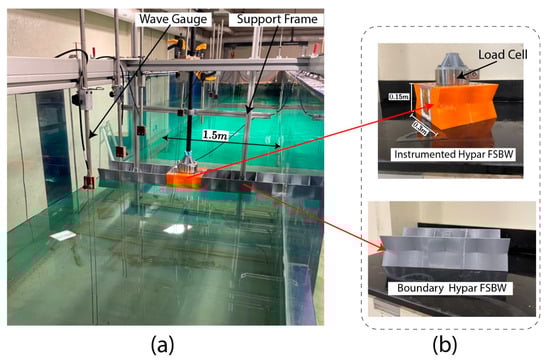
Figure 4.
Experimental setup: (a) Wave flume showing support frame for hypar FSBW, capacitance wave gauges, and load cell. (b) Close-up views of the instrumented hypar FSBW with load cell (top) and boundary hypar FSBW (bottom).

Table 1.
Wave characteristics and FSWB draft used for experimental validation.
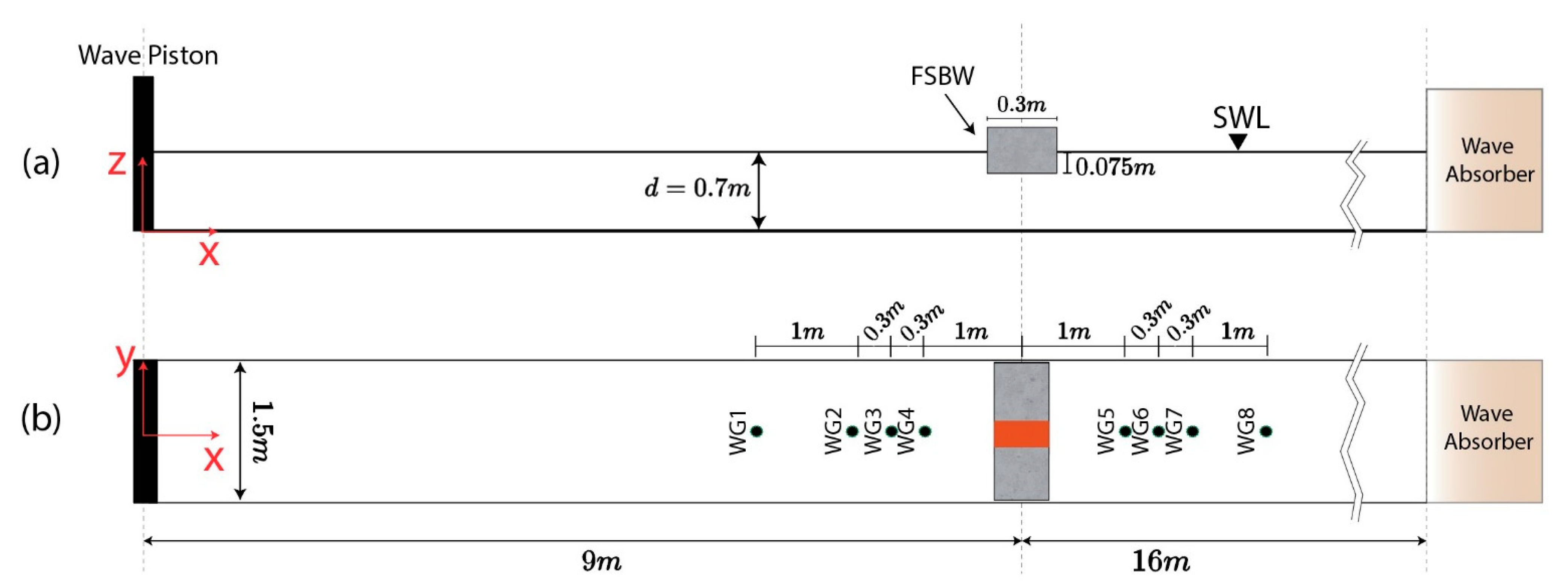
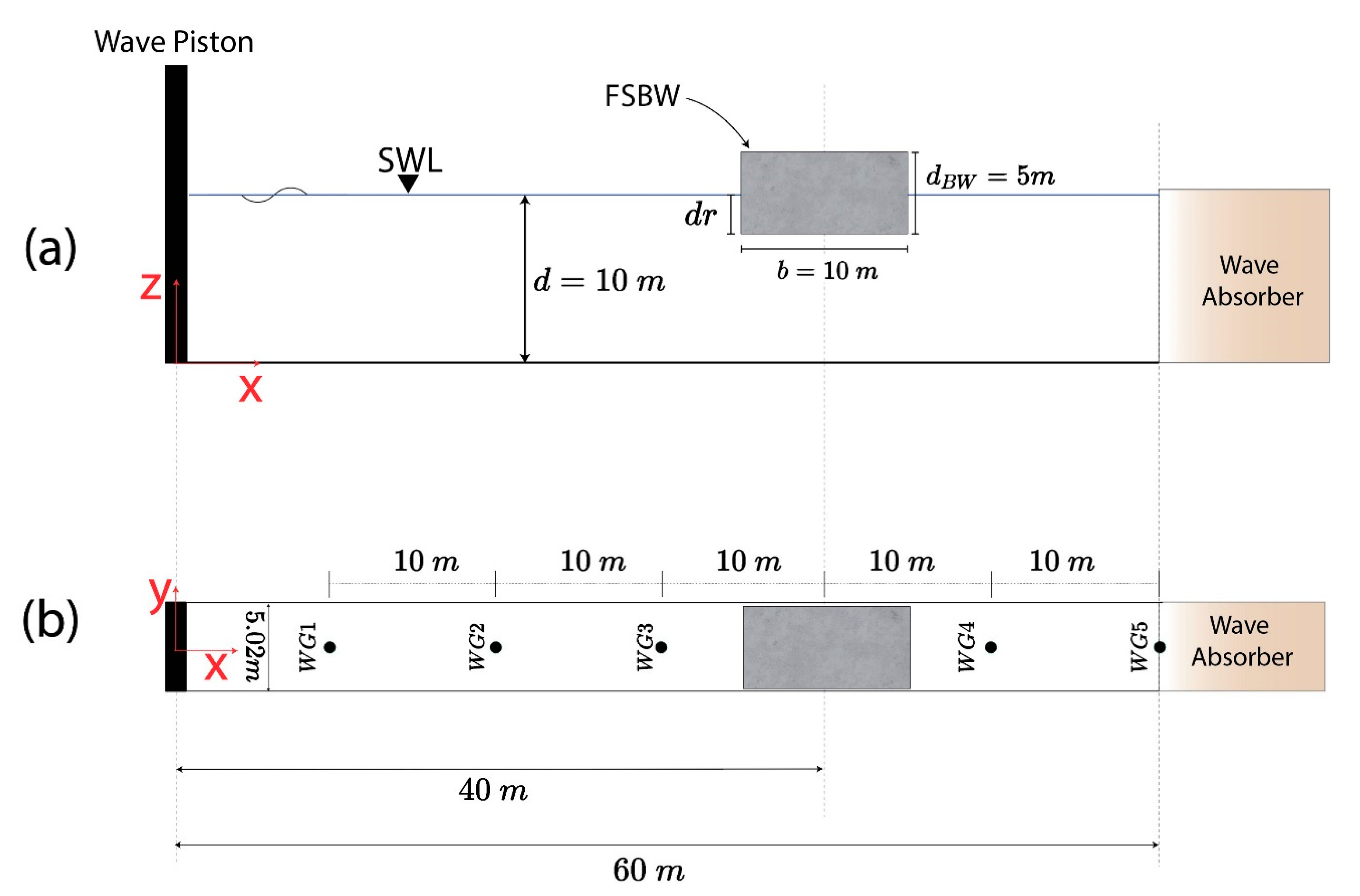
Figure 4 and Figure 5 show the experimental setup. Multiple capacitance wave gauges (WG1 to WG8) along the wave flume were used to measure wave heights at a sampling frequency of 128 Hz. Force measurements were recorded at a sampling frequency of 1000 Hz. A low-pass Butterworth filter [50] was applied to remove the effect of support frame’s natural vibration frequency and high-frequency noise. A hammer test determined the natural frequency of the support frame to be approximately 8 Hz. The low-pass filter effect was found negligible in the current study, likely due to minimal frame vibration amplitude given the submerged FSBW with non-breaking waves.

Figure 5.
Experimental setup: (a) an elevation view, (b) top view.
3.2. SPH Numerical Model
A numerical wave flume, similar to that shown in Figure 4 and Figure 5, was created in DualSPHysics. In the numerical model, however, the flume width was limited to a single hypar FSBW due to computational and memory constraints. Waves are generated by a piston using second order wave theory, as described in Section 2.3. Validation results and numerical simulations settings are presented in the next section.
3.3. Model Validation Study
For initial interparticle distance (), values ranging from 3 mm to 10.8 mm were considered in the sensitivity study for experimental validation. Since the scaled remains constant at 54 mm, this range implies a ratio of wave height to initial interparticle distance ( of 5 to 18. These values fall within the range suggested in the literature, which typically recommends an of 10 [31,38]. The range of is constrained by the computational capabilities [51], i.e., RAM, Graphics Processing Unit (GPU), and storage, with smaller values increasing computational demand [52]. Hence, a balance between accuracy and computational efficiency is required. Note that for the current study, was the finest possible due to computational limits in DualSPHysics.
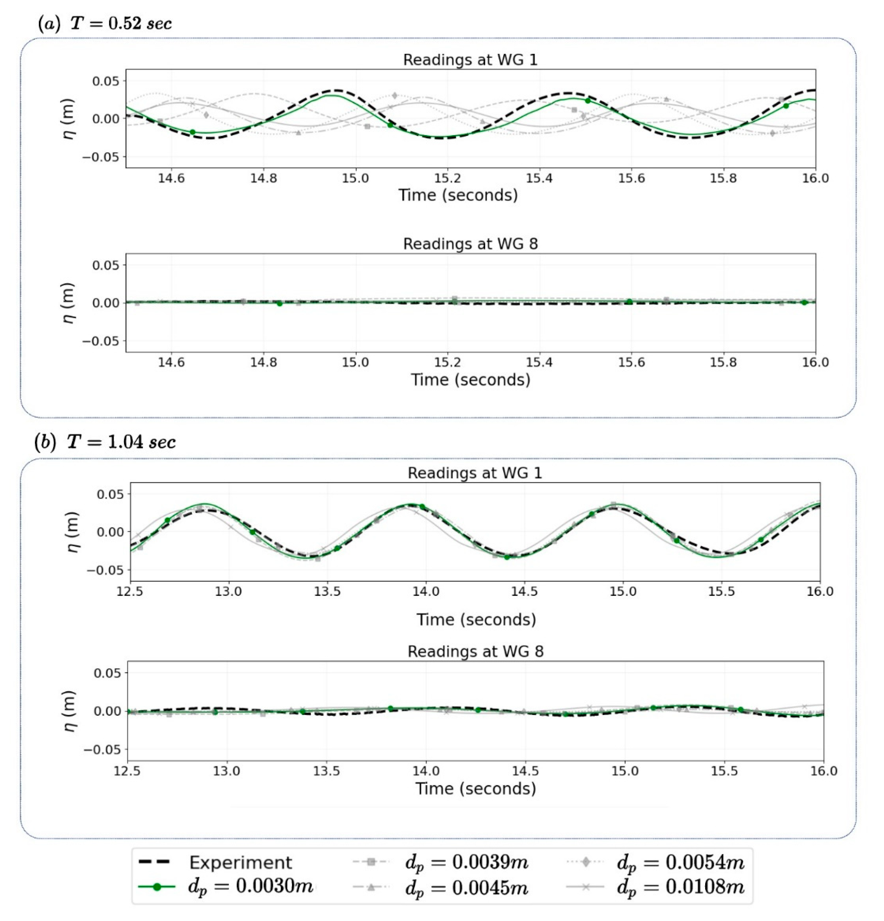
The values were studied by examining wave profiles as shown in Figure 6, which compares experimental and numerical free-surface elevations, , at Wave Gauge 1 (WG1, before the FSBW) and Wave Gauge 8 (WG8, after the FSBW) for wave periods and . The numerical results with the different values generally show good agreement with experimental data, with showing best agreement. To quantify the accuracy, the Root Mean Square Error (RMSE) is calculated between experimental and SPH results [51]:
where is the SPH value, is the experimental value, and is the number of time steps.
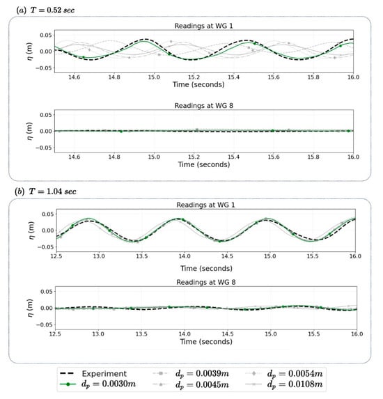
Figure 6.
Comparison of experimental and numerical wave gauge readings for different at two wave periods: (a) T = 0.52 s and (b) T = 1.04 s. The top plots in each panel show readings at Wave Gauge 1 (WG 1), located before the FSBW, while the bottom plots show readings at Wave Gauge 8 (WG 8), positioned after the FSBW.
For and WG1, which represents waves approaching the FSBW, RMSE values were 0.003 m and for and , respectively. These results indicate relatively small deviation and hence, good matching between experimental and SPH incident wave results. Similar results were observed for other wave gauges.
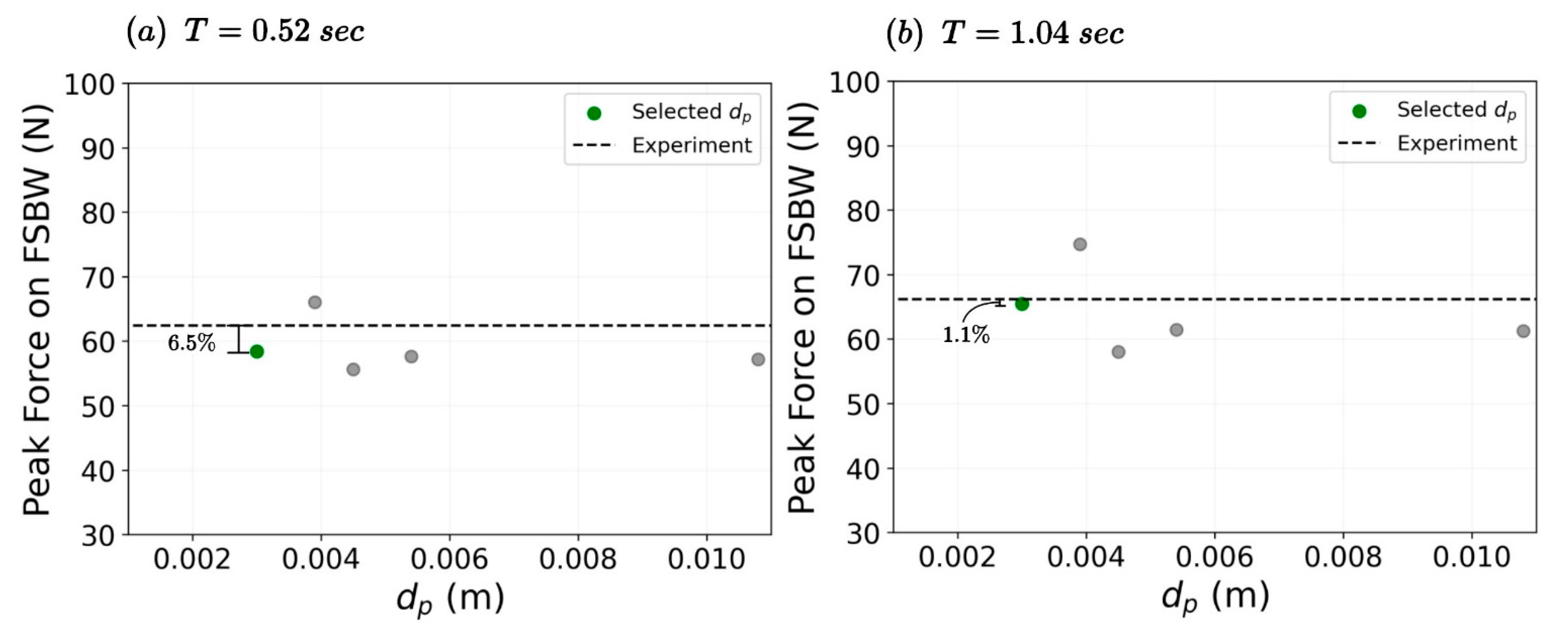
Additionally, different values were studied through force measurements for the same wave periods on the FSBW, with results shown in Figure 7. The SPH simulation with shows the best agreement with experimental data, matching within 6.5% and 1.1% for and , respectively.
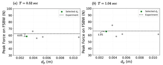
Figure 7.
Peak force on the FSBW model ( for different for two wave periods: (a) T = 0.52 s and (b) T = 1.04 s.
Thus, studies indicate that is a reasonable selection for this study. This value corresponds to (recall , which is finer than the typically recommended ratio of 10 [31,38]. Figure 8 provides additional validation of this selection of Figure 8a shows a visual comparison between experimental observations and SPH visualizations are shown at two-time steps: wave trough and crest at FSBW front for for the selected value. Additionally, Figure 8b presents a time-history comparison of total force between the SPH simulation and experimental results. The comparison reveals good agreement in both the wave profile and the forces during the FSBW interaction.
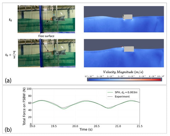
Figure 8.
Comparison of experimental and SPH results for selected : (a) Wave elevation visualization for SPH (right) and experiment (left) during wave interaction ( s) with a hypar FSBW ( at two-time steps: , wave trough at FSBW front, and , half a wave period later where wave crest is at FSBW front. (b) Time-history comparison of total force from SPH and experiment results.
A sensitivity study for the probing distance (see Figure 3) varying from to , indicates that is adequate. Probing pressure too close to the structure boundary resulted in density and pressure fluctuations due to unphysical gaps inherent to SPH, as discussed in previous studies [38,52,53].
Table 2 summarizes the numerical settings used in the parametric study simulations. The simulations required approximately 600 s of real time to simulate 1 s of SPH time. These simulations were executed on high-performance hardware at Princeton Research Computing, utilizing an NVIDIA A100 GPU and an Intel Xeon Platinum 8380 CPU.
Table 2.
SPH numerical simulation and device settings.
4. Parametric Study
4.1. Parameters of the Study
Table 3 presents the geometric parameters selected for this study. The normalized rise describes the warping of the hypar. In the parametric study, three values of were selected: 0 (a flat surface), 0.25, and 0.50. The dimensions of the FSBW, shown in Figure 3b, were selected to be 10 m in length, , and 5 m in depth, , and width, . These parameters were selected to fall within the typical range for FSBW designs [8,15,54], and remained constant in all simulations.
Table 3.
Parameters of the study.
For the FE structural analysis, the hypar surface is discretized into 900 quadrilateral Mindlin/Reissner-type elements with a uniform thickness of 0.25 m, with the selected number of elements being finer than those used in [24,55], which is based on a sensitivity study. Additionally, the hypar surface is assumed to be fixed around its parameter. Given its common application in FSBW [8,15,54], concrete material properties were utilized in this study. High-strength concrete with a compressive strength of 60 MPa and an elastic modulus of 44,000 MPa was selected. The structural analysis assumes an elastic behavior, which is valid for concrete when stresses remain significantly below the failure threshold [56]—a condition that will be demonstrated in the analysis section.
The wave and bathymetry parameters are shown in Table 3. Incident wave periods, , ranging from 3 to 6 s were considered to represent a typical operating range for FSBW [54]. A water depth of 10 m is selected to ensure transitional (or intermediate) to deep wave conditions (see Figure 9). The draft, , was set to two values: 2.5 m (corresponding to the FSBW being half immersed) and 3.5 m (resulting in 70% immersion of the FSBW). All applied waves in this study are second order regular, non-breaking waves with a constant wave height, , of 1.8 m; this wave height is selected to prevent breaking for all waves periods considered and satisfy second order wave maker theory [41,57], as described in Section 2.3.

Figure 9.
Numerical wave flume setup (a) side view and (b) top view.
The numerical setup is illustrated in Figure 9. The configuration consists of a wave piston positioned on the far left, with an Active Wave Absorption System (AWAS) implemented to mitigate wave reflection. The AWAS aims to represent real open sea conditions by eliminating unphysical wave re-reflection [31]. The FSBW is situated 60 m in front of the piston. On the right side of the domain, a 1:10 sloped beach serves as a wave absorber. Wave height along the flume is measured using five wave gauges (WG1 to WG5) installed at different locations, as illustrated in Figure 9b.
4.2. Parametric Study Results
This section presents the results of the parametric study. First, the wave attenuation performance is examined, comparing hypar and flat FSBW designs. Then, for the structural response, the difference in principal stress values between the different designs is analyzed.
4.2.1. Wave Attenuation Performance
The wave transmission coefficient, , was calculated using Equation (7) with the method presented in Section 2.5 and average of wave elevation values taken at WG4 and WG5, on the leeside of the breakwater (see Figure 9).
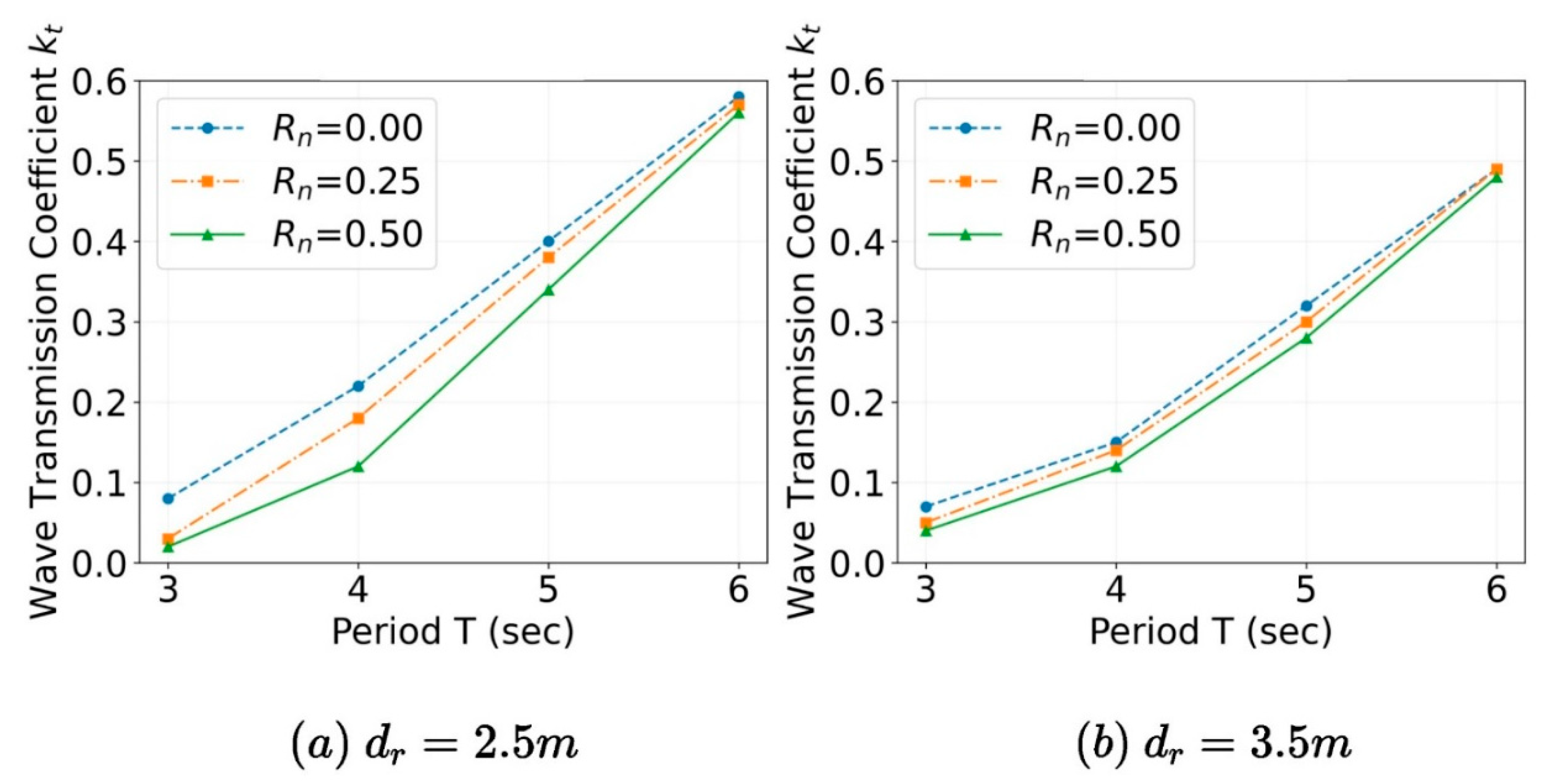
Figure 10 presents the wave transmission coefficient, , results for the hypar FSBW designs across various wave periods and two draft values. For all conditions, increases with the wave period from 3 to 6 s, indicating reduced wave attenuation effectiveness for longer waves. This trend aligns with FSBW performance observed in the literature [15,54,58].
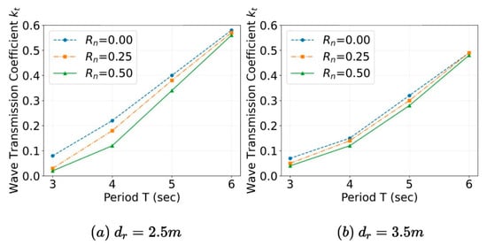
Figure 10.
Wave transmission coefficient, as , values. Results are shown for two draft values: (a) m and (b) .
The draft significantly influences wave attenuation performance. The configurations show lower values compared to the 2.5 m draft across all designs (i.e., values) and wave periods. This observation aligns with previous studies showing that increased immersion depth, or draft, results in better wave attenuation [4,54,58,59]. For the larger draft, , the performance gap between flat and hypar designs narrows, especially for longer wave periods, as shown in Figure 10.
Hypar FSBW designs ( and generally show lower values compared to the flat FSBW (), particularly for shorter wave periods. This improvement is most noticeable for wave periods of 3 and 4 s. Increasing the normalized rise from 0 to 0.50 increases wave attenuation performance, with exhibiting the lowest values. This increased performance is up to 5 times for and , and 1.8 times for and .
There are three possible explanations for how increased warping, , improves wave attenuation performance (i.e., decreases transmission): (1) increased warping may enhance reflection (, Equation (9)), (2) warping may increase wave energy dissipation (, Equation (10)), or (3) both. For and , average wave elevation measurements are taken at WG1 and WG2, located in front of the breakwater. Refer to Section 2.5 for further details. Note that WG3 wave reflection readings were generally found to be unreliable for because the wave gauge is too close, relative to wavelength, to the FSBW.
To determine the primary wave attenuation mechanism, reflection and dissipation are evaluated and compared for different warping values. Three scenarios are considered: (1) which demonstrates the best relative performance of the hypar compared to a flat surface as shown in Figure 10; (2) (which is like the first scenario but a larger draft), and (3) (which is like the first scenario but a larger period). The results for these cases are summarized in Table 4.
Table 4.
Transmission, reflection, and dissipation coefficients for different warping values for representative wave scenarios.
For scenario 1 ( and , hypar surface () shows significantly better attenuation performance compared to flat surface (), where smaller indicates better performance. The reflection coefficient for the flat surface () is around 0.76 which decreases to 0.40 for hypar surface (). Therefore, reflection cannot explain why the hypars exhibit better wave attenuation. The wave dissipation coefficients for the above-mentioned wave scenario, indicate that dissipation increases with warping. In particular, dissipation coefficient is 0.61 for and reaches up to 0.91 for .
The same observation—that increased warping enhances dissipation—applies to scenario 2, which has the same wave period ( but a larger draft ( compared to scenario 1. In scenario 2, although transmission slightly decreases from 0.15 to 0.12 as increases from 0.00 to 0.50, dissipation increases substantially from 0.64 to 0.89 over the same range of . For scenario 3, which differs from case 1 by an increased wave period ( and, consequently, a longer wavelength while maintaining the same draft (, wave attenuation is primarily driven by dissipation regardless of the warping value; increases only slightly, from 0.91 to 0.94, as increases from 0.00 to 0.50.
Table 4 thus indicates that the improved attenuation performance of the hypar FSBW can be attributed to wave dissipation induced by the hypar curvature. Further, these results indicate that the relative wave dissipation efficiency of the hypar compared to a flat surface depends more on wavelength (obtained from wave period) and less on the draft, within the range of the study parameters.
4.2.2. Structural Response
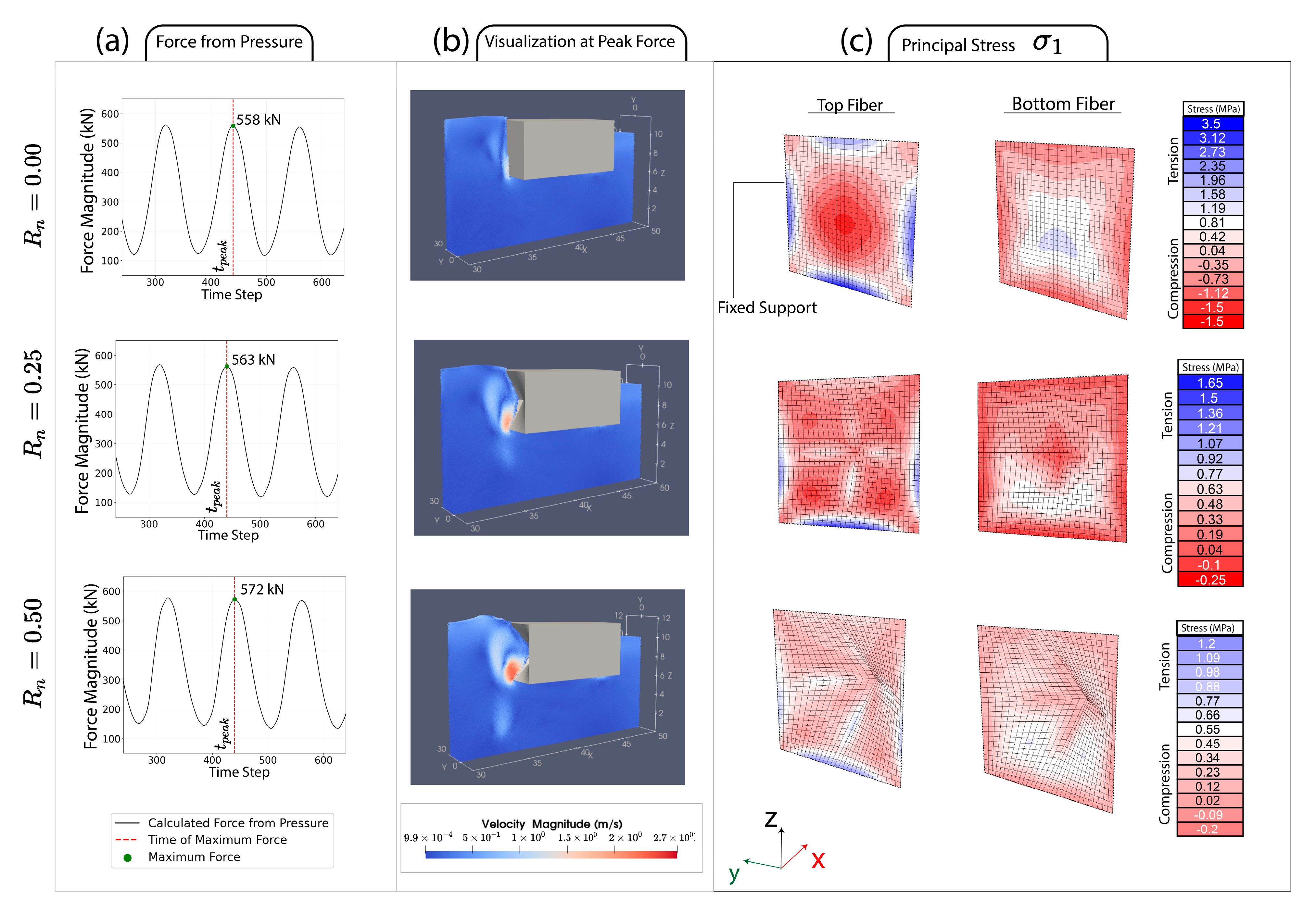
The structural response of the FSBW designs under peak-static and dynamic wave loading was analyzed by examining the maximum principal stress values. For instance, Figure 11 shows maximum principal stress distribution, , for varying normalized rise, , values, under a wave period of and a draft of . This wave scenrio is critical, as it resulted in the largest stresses in the FSBW compared to the other period and draft scenarios. For the flat FSBW (), a single region of high compression stress is observed slightly below the center of the top surface, with maximum tensile and compressive stresses of around and , respectively. As increases to 0.25 and 0.50, the compression stress shifts to two regions of lower magnitude stresses closer to the bottom corners. For , the maximum tensile stress reduces to 1.2 MPa and the maximum compressive stress to −0.20 MPa, indicating a significant stress reduction compared to the flat design—specifically 3 times lower for tension and 7.5 times for compression on the top surface. The trends shown in Figure 11 are the same for other wave scenarios. Indeed, stress values are dependent on thickness, and these results are for a shell thickness of 25 cm. Next, the effect of thickness on stress values, which informed the choice of thickness value, is presented.

Figure 11.
Comparison of structural response for FSBW designs with varying normalized rise, , for a wave period and draft, , and shell thickness = 25 cm: (a) time-history of force acting on FSBW surface, (b) SPH visualization at peak force, and (c) principal stress distribution on the top and bottom fibers of the FSBW surface.
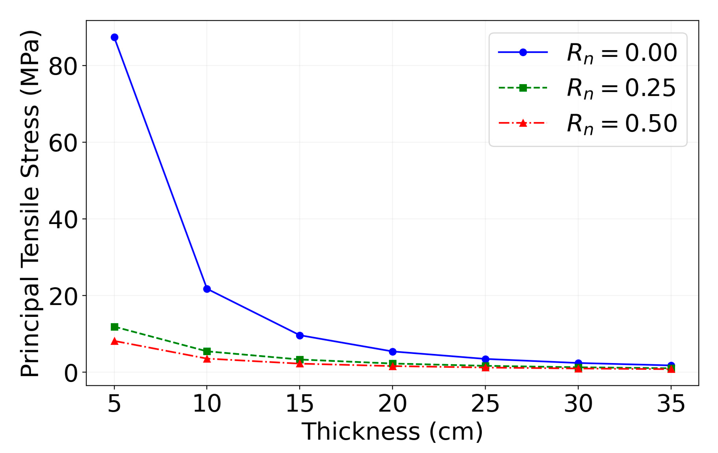
Elastic analyses were conducted to examine the effect of varying FSBW thickness on the maximum principal tensile stress for different under critical wave scenario, i.e., T = 6 and , with the results shown in Figure 12. The flat FSBW () consistently exhibits the highest stress levels across all thicknesses, while the hypar designs ( and ) show significantly lower stress levels especially at smaller thickness, , value; for example, at a thickness , the tensile stress for is around 13 times lower than for . Additionally, while increasing from 0.25 to 0.5 further decreases stress, this effect is less significant. For instance, for , decreasing from 0.00 to 0.25 results in 8 times lower tensile stress, but increasing further from 0.25 to 0.5 only reduces tensile stress by a factor of 1.6. The same trend of higher resulting in lower principal stresses is observed for other materials (specifically aluminum and steel) under elastic assumption as well as for the other draft value .
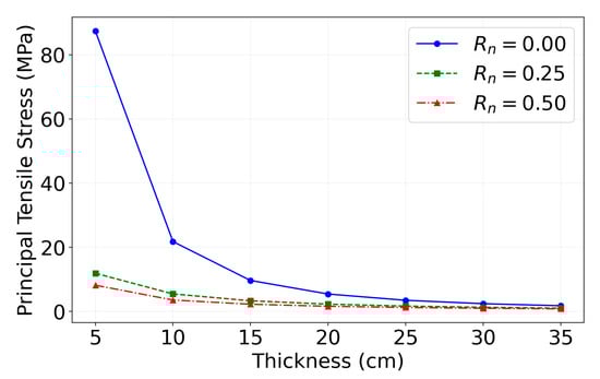
Figure 12.
Maximum principal tensile stress, , as a function of FSBW thickness for different normalized rise, , values for and .
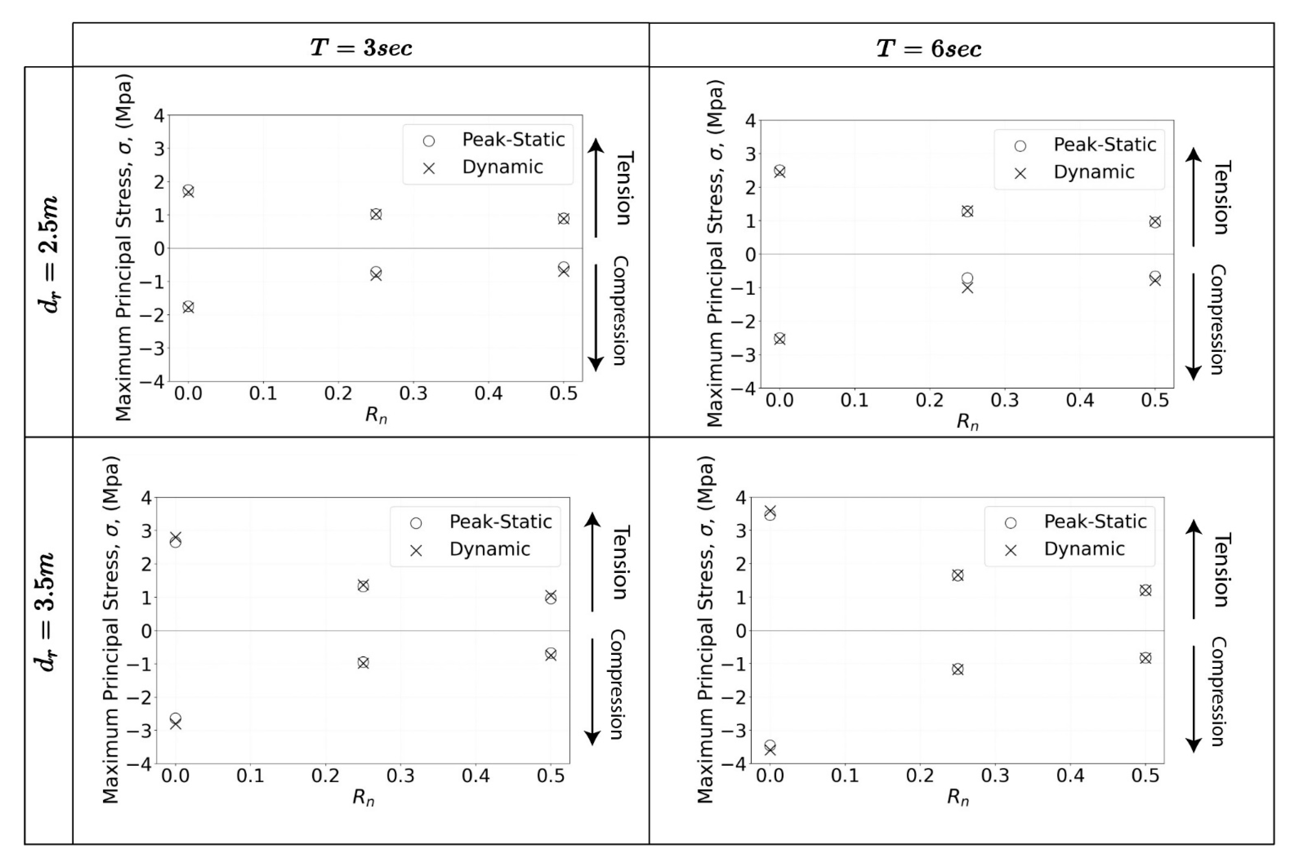
Figure 13 shows the dynamic effects of wave loading conditions by comparing the maximum principal stress values for different to peak-static values for wave periods of and and drafts and . It is seen that although the dynamic analysis results in higher stress values compared to static analysis, the difference on average is less than 6%. This suggests that a static analysis provides a reasonable approximation for hypar FSBW preliminary design under the regular wave conditions studied herein, a conclusion previously presented by Wu et al. [24]. In addition, the stress values presented under all conditions for FSBW with a thickness of 25 cm are well below the assumed compressive strength of 60 MPa (tensile strength assumed to equal approximately one-tenth of the compressive strength), validating the applicability of elastic analysis [56].

Figure 13.
Comparison of peak-static and dynamic loading conditions via maximum principal stress, , for different normalized rise, ,values (shell thickness .
In all cases, increasing results in a substantial reduction in maximum principal stress magnitudes, in both tension and compression. For instance, for and , the maximum tensile stress decreases from 2.8 MPa for to 1.4 MPa for = 0.25, a 2 times reduction. For and , the reduction is from about 3.6 MPa to 1.7 MPa, a similar 2 times reduction. However, as increases from 0.25 to 0.50, the maximum tensile stress decreases from 1.4 MPa to 1.1 MPa, representing only a 1.3 times reduction for and . Similarly, for and , the reduction is from 1.7 MPa to 1.2 MPa, a 1.4 times decrease. This indicates that the stress reduction effect of increasing warping diminishes as becomes larger, as was previously observed in thickness study in Figure 12. Additionally, the same trend is evident for the smaller draft value, . Principal compressive stresses exhibit a similar trend.
5. Summary and Conclusions
This study analyzed the performance of Free-Surface Breakwaters (FSBW) with hypar-faces of varying warping values across various wave characteristics. Experimental studies validated numerical simulations used in a parametric study that investigated the potential of hypar geometry in FSBW for enhancing wave attenuation and structural efficiency via a decoupled SPH-FEM analysis. Wave attenuation performance was examined through the wave transmission coefficient, while structural response was analyzed through comparing principal stress values. The conclusions drawn from this study are:
- Hypar-faced FSBW designs improve wave attenuation performance compared to flat-faced designs, primarily through wave dissipation. The improved performance is more pronounced for shorter wave periods and lower draft values.
- Hypar geometry significantly reduces maximum principal stress values compared to flat designs. This effect is most pronounced for FSBWs with thinner shell walls.
- Peak-static analysis provides a reasonable approximation for the structural stresses of hypar FSBW under regular wave conditions, with less than 6% difference from dynamic analysis results.
While this study provides valuable insights into the potential of hypar-faced FSBW, it is noted that the study was limited to regular waves with a constant height, and one material, concrete, which did not account for long-term effects or environmental degradation. Regardless, the findings still remain significant. Since the wave period (or wavelength) is identified as the primary factor influencing wave attenuation [8,38,59], the results cover the performance of hypar FSBWs across a wide range of wave conditions, potentially providing insight about behavior under irregular waves. Additionally, the elastic assumption used in the analysis ensures that the conclusions are applicable to other materials, as stress values remain essentially unaffected under elastic behavior.
Despite its limitations, the study demonstrates the practical benefits of hypar FSBWs, including improved wave attenuation and reduced structural stresses, and it encourages further examination of hypar-faced FSBWs as efficient and effective breakwaters that reduce both attenuation and structural stresses.
Author Contributions
S.S.: conceptualization, methodology, software, validation, formal analysis, writing—original draft, review and editing. G.W.: conceptualization, methodology, software, validation, formal analysis, review and editing. K.A.P.: conceptualization, validation, review and editing. M.G.: conceptualization, validation, writing—review and editing, supervision, funding acquisition. All authors have read and agreed to the published version of the manuscript.
Funding
This work was funded by Project X at Princeton University and the National Science Foundation (NSF) under grant CMMI-2227489. All opinions expressed in this paper are the authors’ and do not necessarily reflect the policies and views of the sponsors.
Institutional Review Board Statement
Not applicable.
Informed Consent Statement
Not applicable.
Data Availability Statement
The data used for this paper is publicly available at the following repository: https://github.com/hse95/Hypar-FSBW.
Acknowledgments
The authors thank Ali Farhadzadeh, Tao Xiang (Stony Brook University), and Zhaoyang Song (Princeton University) for their valuable insights and support.
Conflicts of Interest
The authors declare no conflicts of interest.
References
- Vardy, M.; Oppenheimer, M.; Dubash, N.K.; O’Reilly, J.; Jamieson, D. The intergovernmental panel on climate change: Challenges and opportunities. Annu. Rev. Environ. Resour. 2017, 42, 55–75. [Google Scholar] [CrossRef]
- Pérez-Alarcón, A.; Fernández-Alvarez, J.C.; Coll-Hidalgo, P. Global Increase of the Intensity of Tropical Cyclones Under Global Warming Based on Their Maximum Potential Intensity and CMIP6 Models. Environ. Process. 2023, 10, 36. [Google Scholar] [CrossRef]
- Rambabu, N.; Srineash, V. A Review on Methodologies to Upgrade the Coastal Structures to Enhance the Coastal Resilience. In Proceedings of the OCEANS 2022-Chennai, Chennai, India, 21–24 February 2022; pp. 1–9. [Google Scholar]
- Teh, H. Hydraulic performance of free surface breakwaters: A review. Sains Malays. 2013, 42, 1301–1310. [Google Scholar]
- Lorenzoni, C.; Soldini, L.; Brocchini, M.; Mancinelli, A.; Postacchini, M.; Seta, E.; Corvaro, S. Working of defense coastal structures dissipating by macroroughness. J. Waterw. Port Coast. Ocean. Eng. 2010, 136, 79–90. [Google Scholar] [CrossRef]
- He, F. Experimental Investigation of Pile-Supported/Floating Breakwaters Integrated with Oscillating-Water-Column Converters. Ph.D. Thesis, Nanyang Technological University, Singapore, 2013. [Google Scholar]
- Isaacson, M.; Whiteside, N.; Gardiner, R.; Hay, D. Modelling of a circular-section floating breakwater. Can. J. Civ. Eng. 1995, 22, 714–722. [Google Scholar] [CrossRef]
- Elchahal, G.; Lafon, P.; Younes, R. Design optimization of floating breakwaters with an interdisciplinary fluid–solid structural problem. Can. J. Civ. Eng. 2009, 36, 1732–1743. [Google Scholar] [CrossRef]
- Brossard, J.; Jarno-Druaux, A.; Marin, F.; Tabet-Aoul, E. Fixed absorbing semi-immersed breakwater. Coast. Eng. 2003, 49, 25–41. [Google Scholar] [CrossRef]
- Günaydın, K.; Kabdaşlı, M. Performance of solid and perforated U-type breakwaters under regular and irregular waves. Ocean. Eng. 2004, 31, 1377–1405. [Google Scholar] [CrossRef]
- Wang, Y.; Wang, G.; Li, G. Experimental study on the performance of the multiple-layer breakwater. Ocean. Eng. 2006, 33, 1829–1839. [Google Scholar] [CrossRef]
- Sundar, V. Hydrodynamic pressures and forces on quadrant front face pile supported breakwater. Ocean. Eng. 2002, 29, 193–214. [Google Scholar] [CrossRef]
- Koutandos, E.; Prinos, P. Hydrodynamic characteristics of semi-immersed breakwater with an attached porous plate. Ocean. Eng. 2011, 38, 34–48. [Google Scholar] [CrossRef]
- Lv, C.; Zhao, X.; Zheng, K.; Zong, Y.; Zheng, S.; Jiang, H.; Yao, S.; Luan, H. Hydrodynamic performance of a floating fluid-filled membrane breakwater: Experimental and numerical study. J. Fluid Mech. 2024, 1001, A21. [Google Scholar] [CrossRef]
- Elchahal, G.; Younes, R.; Lafon, P. Optimization of coastal structures: Application on detached breakwaters in ports. Ocean. Eng. 2013, 63, 35–43. [Google Scholar] [CrossRef]
- Cebada-Relea, A.J.; López, M.; Claus, R.; Aenlle, M. Short-term analysis of extreme wave-induced forces on the connections of a floating breakwater. Ocean. Eng. 2023, 280, 114579. [Google Scholar] [CrossRef]
- Wang, S.; Garlock, M.; Glisic, B. Geometric and area parameterization of N-edged hyperbolic paraboloidal umbrellas. Eng. Struct. 2022, 250, 113499. [Google Scholar] [CrossRef]
- ElDarwich, H.; Mansouri, I.; Garlock, M.; Wang, S. Predicting Maximum Deflection of N-Edged Thin-Shelled Hyperbolic-Paraboloid Umbrella Using Machine Learning Techniques. Thin-Walled Struct. 2024, 205, 112412. [Google Scholar] [CrossRef]
- Gergely, P.; Banavalkar, P.V.; Parker, J.E. The Analysis and Behavior of Thin-Steel Hyperbolic Paraboloid Shells; Report No. 338; Wei-Wen Yu Center for Cold-Formed Steel Structures, Civil, Architectural and Environmental Engineering Department, Missouri University of Science and Technology: Rolla, MO, USA, 1971. [Google Scholar]
- Garlock, M.E.M.; Billington, D.P. Félix Candela: Engineer, Builder, Structural Artist; Princeton University Art Museum: Princeton, NJ, USA; Yale University Press: New Haven, CT, USA, 2008. [Google Scholar]
- Wang, S.; Garlock, M.; Deike, L.; Glisic, B. Feasibility of Kinetic Umbrellas as deployable flood barriers during landfalling hurricanes. J. Struct. Eng. 2022, 148, 04022047. [Google Scholar] [CrossRef]
- Wang, S.; Garlock, M.; Glisic, B. Kinematics of deployable hyperbolic paraboloid umbrellas. Eng. Struct. 2021, 244, 112750. [Google Scholar] [CrossRef]
- Wang, S.; Notario, V.; Garlock, M.; Glisic, B. Parameterization of hydrostatic behavior of deployable hypar umbrellas as flood barriers. Thin-Walled Struct. 2021, 163, 107650. [Google Scholar] [CrossRef]
- Wu, G.; Garlock, M.; Wang, S. A decoupled SPH-FEM analysis of hydrodynamic wave pressure on hyperbolic-paraboloid thin-shell coastal armor and corresponding structural response. Eng. Struct. 2022, 268, 114738. [Google Scholar] [CrossRef]
- ElDarwich, H.S.; Pawitan, K.A.; Garlock, M.E. Conceptual Investigation on the Effectiveness of Hyperbolic Paraboloid Surfaces for Floating Breakwaters. In Proceedings of the IASS 2022 Symposium Affiliated with APCS 2022 Conference, Beijing, China, 19–23 September 2022, ISSN 2518-6582. [Google Scholar]
- Antoci, C.; Gallati, M.; Sibilla, S. Numerical simulation of fluid–structure interaction by SPH. Comput. Struct. 2007, 85, 879–890. [Google Scholar] [CrossRef]
- McNeel, R. Rhinoceros 3D, Version 7 2020. Robert McNeel & Associates, Seattle, WA, USA, 2015. Available online: https://www.rhino3d.com.
- Crespo, A.; Domínguez, J.; Rogers, B.; Gómez-Gesteira, M.; Longshaw, S.; Canelas, R.; Vacondio, R.; Barreiro, A.; García-Feal, O. DualSPHysics: Open-source parallel CFD solver based on Smoothed Particle Hydrodynamics (SPH). Comput. Phys. Commun. 2015, 187, 204–216. [Google Scholar] [CrossRef]
- CSI. SAP2000 CSI Analysis Reference Manual 2014; Computers and Structures, Inc.: Walnut Creek, CA, USA, 2014; Available online: https://www.csiamerica.com.
- Monaghan, J.J. Smoothed particle hydrodynamics. Rep. Prog. Phys. 2005, 68, 1703. [Google Scholar] [CrossRef]
- Altomare, C.; Domínguez, J.; Crespo, A.; González-Cao, J.; Suzuki, T.; Gómez-Gesteira, M.; Troch, P. Long-crested wave generation and absorption for SPH-based DualSPHysics model. Coast. Eng. 2017, 127, 37–54. [Google Scholar] [CrossRef]
- Martínez-Estévez, I.; Tagliafierro, B.; El Rahi, J.; Domínguez, J.; Crespo, A.; Troch, P.; Gómez-Gesteira, M. Coupling an SPH-based solver with an FEA structural solver to simulate free surface flows interacting with flexible structures. Comput. Methods Appl. Mech. Eng. 2023, 410, 115989. [Google Scholar] [CrossRef]
- Wendland, H. Piecewise polynomial, positive definite and compactly supported radial functions of minimal degree. Adv. Comput. Math. 1995, 4, 389–396. [Google Scholar] [CrossRef]
- Fourtakas, G.; Vacondio, R.; Alonso, J.D.; Rogers, B.D. Improved Density Diffusion Term for Long Duration Wave Propagation. In Proceedings of the 2020 SPHERIC Harbin International Workshop, Harbin, China, 13 January–16 September 2020. [Google Scholar]
- Grubmüller, H.; Heller, H.; Windemuth, A.; Schulten, K. Generalized Verlet algorithm for efficient molecular dynamics simulations with long-range interactions. Mol. Simul. 1991, 6, 121–142. [Google Scholar] [CrossRef]
- Monaghan, J.J.; Cas, R.A.; Kos, A.; Hallworth, M. Gravity currents descending a ramp in a stratified tank. J. Fluid Mech. 1999, 379, 39–69. [Google Scholar] [CrossRef]
- Batchelor, G.K. An Introduction to Fluid Dynamics, 1st ed.; Cambridge University Press: Cambridge, UK, 2000. [Google Scholar] [CrossRef]
- Liu, Z.; Wang, Y. Numerical studies of submerged moored box-type floating breakwaters with different shapes of cross-sections using SPH. Coast. Eng. 2020, 158, 103687. [Google Scholar] [CrossRef]
- Wu, G.; Garlock, M. Investigating the effects of box girder bridge geometry on solitary wave force using SPH modeling. Coast. Eng. 2024, 187, 104430. [Google Scholar] [CrossRef]
- Cabrera Crespo, A.J.; Gómez Gesteira, R.; Dalrymple, R.A. Boundary conditions generated by dynamic particles in SPH methods. Comput. Mater. Contin. 2007, 5, 173–184. [Google Scholar]
- Madsen, O.S. On the generation of long waves. J. Geophys. Res. 1971, 76, 8672–8683. [Google Scholar] [CrossRef]
- Estevez, I.M. Coupling Between the DualSPHysics Solver and Multiphysics Libraries: Implementation, Validation and Real Engineering Applications. Ph.D. Thesis, Universidade of Vigo, Pontevedra, Spain, 2024. [Google Scholar]
- Pawitan, K.A. Wave Loadings and Scaling Effects on, and Within, an Oscillating Water Column (OWC) Caisson Breakwater. Ph.D. Thesis, University of Edinburgh, Edinburgh, UK, 2019. [Google Scholar]
- Zago, V.; Schulze, L.J.; Bilotta, G.; Almashan, N.; Dalrymple, R. Overcoming excessive numerical dissipation in SPH modeling of water waves. Coast. Eng. 2021, 170, 104018. [Google Scholar] [CrossRef]
- Mathisen, J.; Bitner-Gregersen, E. Joint distributions for significant wave height and wave zero-up-crossing period. Appl. Ocean. Res. 1990, 12, 93–103. [Google Scholar] [CrossRef]
- Goda, Y.; Suzuki, Y. Estimation of incident and reflected waves in random wave experiments. Coast. Eng. 1976, 1976, 828–845. [Google Scholar] [CrossRef]
- Newmark, N.M. A method of computation for structural dynamics. J. Eng. Mech. Div. 1959, 85, 67–94. [Google Scholar] [CrossRef]
- Hughes, S.A. Physical Models and Laboratory Techniques in Coastal Engineering, 7th ed.; World Scientific: Singapore, 1993. [Google Scholar] [CrossRef]
- Munson, B.R.; Okiishi, T.H.; Huebsch, W.W.; Rothmayer, A.P. Fundamentals of Fluid Mechanics, 7th ed.; John Wiley & Sons, Inc.: Hoboken, NJ, USA, 2013. [Google Scholar]
- Butterworth, S. On the theory of filter amplifiers. Wirel. Eng. 1930, 7, 536–541. [Google Scholar]
- Reis, C.; Barbosa, A.R.; Figueiredo, J.; Clain, S.; Lopes, M.; Baptista, M.A. Smoothed particle hydrodynamics modeling of elevated structures impacted by tsunami-like waves. Eng. Struct. 2022, 270, 114851. [Google Scholar] [CrossRef]
- Domínguez, J.; Fourtakas, G.; Cercós-Pita, J.; Vacondio, R.; Rogers, B.D.; Crespo, A. Evaluation of reliability and efficiency of different boundary conditions in a SPH code. In Proceedings of the 10th International SPHERIC Workshop, Parma, Italy, 16–18 June 2015. [Google Scholar]
- Ferrand, M.; Laurence, D.R.; Rogers, B.D.; Violeau, D.; Kassiotis, C. Unified semi-analytical wall boundary conditions for inviscid, laminar or turbulent flows in the meshless SPH method. Int. J. Numer. Methods Fluids 2013, 71, 446–472. [Google Scholar] [CrossRef]
- Dai, J.; Wang, C.M.; Utsunomiya, T.; Duan, W. Review of recent research and developments on floating breakwaters. Ocean. Eng. 2018, 158, 132–151. [Google Scholar] [CrossRef]
- Wang, S.; Garlock, M.; Glisic, B. Hydrostatic Response of Deployable Hyperbolic-Paraboloid Umbrellas as Coastal Armor. J. Struct. Eng. 2020, 146, 04020096. [Google Scholar] [CrossRef]
- Robutti, G.; Ronzoni, E.; Ottosen, N. Failure Strength and Elastic Limit for Concrete: A Comparative Study. In Proceedings of the 5th International Conference on Structural Mechanics in Reactor Technology, Berlin, Germany, 12–16 August 1979. [Google Scholar]
- Le Méhauté, B.; Koh, R.C.Y. On the Breaking of Waves Arriving at an Angle to the Shore. J. Hydraul. Res. 1967, 5, 67–88. [Google Scholar] [CrossRef]
- Martin, W.; Adee, B.H. Theoretical Analysis of Floating Breakwater Performance. In Proceedings of the Fifth Indian National Conference on Harbour and Ocean Engineering, Goa, India, 4–6 February 1974. [Google Scholar]
- Macagno, E. Fluid mechanics: Experimental study of the effects of the passage of a wave beneath an obstacle. In Proceedings of the Academic Des Sciences, Paris, France, 28 February 1953. [Google Scholar]


Disclaimer/Publisher’s Note: The statements, opinions and data contained in all publications are solely those of the individual author(s) and contributor(s) and not of MDPI and/or the editor(s). MDPI and/or the editor(s) disclaim responsibility for any injury to people or property resulting from any ideas, methods, instructions or products referred to in the content. |
© 2025 by the authors. Licensee MDPI, Basel, Switzerland. This article is an open access article distributed under the terms and conditions of the Creative Commons Attribution (CC BY) license (https://creativecommons.org/licenses/by/4.0/).