Abstract
Mesoscale eddies are known to influence the abundance and distribution of oceanic cephalopods. However, little is known about these effects in the southwest Atlantic Ocean. Therefore, this study analyzed the variations in environmental conditions and the resource abundance, spatial distribution, and habitat suitability of Illex argentinus within different life stages of cyclonic (CE) and anticyclonic (AE) eddies in Patagonian waters. From a comparison of squid abundance between CEs and AEs at each life stage, it was found that I. argentinus gradually increased in abundance after eddy formation, that abundance peaked during eddy maturation and that it subsequently decreased during the eddies’ decay phase. Spatially, squid resources in AEs were primarily concentrated in the northwest and southeast peripheral regions of the eddy, while in CEs, resources were more concentrated in the outer regions, on the western side of the eddy. Environmental factor analysis revealed that sea surface temperature (SST) and temperature at 200 m depth (T200m) in both CEs and AEs reached their lowest values during the intensification and maturation phases of the eddies. Chlorophyll a (Chl-a) concentrations were significantly higher in CEs than in AEs from the formation to the maturation phase; however, during eddy decay, Chl-a concentrations were higher in AEs. According to a comparison of the suitability index (SI) for each environmental factor and the habitat suitability index (HSI) model, SISST, SIT200m, and SIChl-a in AEs increased and then decreased with eddy evolution, with optimal SI values occurring during the intensification phase. In CEs, SISST and SIT200m also increased and then decreased, with optimal SISST and SIT200m occurring during the intensification and maturation phases, respectively, with little variation in SIChl-a across the life cycle of CEs. The HSI in both types of eddies gradually increased from the formation phase, reached a peak during maturation, and significantly decreased during eddy decay. Overall, this study indicated that habitat suitability and resource abundance for I. argentinus were highest during the maturation phase of the eddies.
1. Introduction
Mesoscale eddies are ubiquitous dynamic oceanic processes that are typically generated by environmental instability, topography, wind fields, and ocean currents [1,2,3]. The lifespan of these eddies ranges from days to months, with a radiative range of 10–200 km and an impact depth reaching up to 1000 m [4,5,6]. In the Southern Hemisphere, cyclonic eddies (CE) rotate clockwise, while anticyclonic eddies (AE) rotate counterclockwise. In CEs, or (1) cold eddies, cold water is upwelled to the upper water layers, resulting in lower temperatures at the eddy core. In AEs, or warm eddies, downwelling of warm surface water leads to higher temperatures at the core [7,8]. The edges of AEs and the centers of CEs possess dynamic downwelling and upwelling systems, respectively, making them regions of enhanced productivity. Nutrient-rich upwelling at the cores of CEs increases productivity and food availability for mesopelagic organisms, while the transport of warm surface water to deeper layers within AEs provides favorable conditions for plankton to inhabit greater depths.
Marine mesoscale eddies and other dynamic oceanographic characteristics are associated with changes in the vertical structure of plankton communities. These systems can regulate physiological activities and food supply, attracting more fish and promoting frequent fishing activities in these areas. This phenomenon is commonly observed in cephalopod species and fishes such as neon flying squid Ommastrephes bartramii in the northwest Pacific Ocean [9], as well as in the swordfish in the northwest Atlantic [10] and white sharks in the Gulf Stream and Sargasso Sea [11]. In general, CEs are less productive than AEs [8,12]; however, the ecological effects of mesoscale eddies are complex, as the primary bio-physical mechanisms vary across oceanic regions and habitat preferences vary across species. Thus, the impact of mesoscale eddies on the distribution of high-trophic organisms remains less understood. In this context, preliminary studies in the Kuroshio Current system [13], the Gulf Stream system [14], the eastern Pacific [15], and the South China Sea [16] have shown that oceanic productivity is higher near eddy regions. Mesoscale eddies regulate the distribution of chlorophyll at the eddy edges and seawater temperature and nutrients within the eddy through the horizontal and vertical movements of ocean currents, significantly impacting primary productivity and thus the marine environment.
Illex argentinus is an oceanic shallow-water species and is one of the most globally important cephalopod resources. It primarily feeds on crustaceans, fish, and other cephalopods and is widely distributed in the southwestern Atlantic Ocean between 22° and 54º S, around the continental shelf and slope areas [17,18]. It inhabits the water column from the sea surface to 800 m depth, forming dense aggregations between 50 and 200 m depth on the continental shelf during autumn and winter [19]. Illex argentinus is characterized by rapid growth, a short life cycle, and high population differentiation, making it a typical opportunistic feeding group [20]. Although the species is highly sensitive to environmental changes, these traits also enable the species to respond quickly to climate or environmental changes compared to other species. Oceanographic variability at both spawning and hatching grounds is crucial for determining the contribution of this species as a fisheries resource.
Mesoscale eddies are prominent in Patagonian waters, where I. argentinus aggregates in highly productive areas such as frontal zones, the Malvinas Current, the Brazil Current, and areas where cold and warm currents converge. The complex and unstable current systems and the vast continental slope in Patagonian waters [4,21] provide favorable conditions for the formation of mesoscale eddies that can directly regulate the distribution of I. argentinus. Previous studies have focused on the impact of the marine environment and ocean currents on the abundance of I. argentinus [22,23] and on changes in their growth and reproduction [24,25]; however, few have investigated how mesoscale eddies regulate the abundance and spatial distribution of this species at different eddy life stages. Therefore, based on previous classifications of eddy life cycles [26,27], this study assessed the abundance and spatial distribution of Argentine shortfin squid during different life stages of both CEs and AEs, with a focus on environmental shifts within the eddy life cycles, to determine the ecological response of this species and how its habitat may shift. This study selected six long-lived mesoscale eddies with complete life cycles as case studies, aiming to provide a scientific basis for the sustainable use and management of I. argentinus resources in Patagonian waters.
2. Materials and Methods
2.1. Fisheries Data
Fishing data on I. argentinus from 1 January to 30 April between 2013 to 2019 were obtained from the China Distant-Water Fisheries Data Center at Shanghai Ocean University. The study took place offshore from Patagonia, in the southwestern Atlantic Ocean, spanning 70° to 50°W and 55° to 35°S. The dataset comprised a total of 68,288 original fishing locations and included location (longitude and latitude), fishing date (year, month, day), fishing effort (days), and catch (tons). To enhance the precision of grid-based processing of fisheries and eddy data, we standardized the spatial resolution of all fisheries data to 1/4°. The catch per unit effort (CPUE, tons/day) for each original fishing location was calculated, with CPUE ≥ 5 used as an indicator of high resource abundance. The total occurrences of CPUE ≥ 5 at each original fishing location were subsequently calculated using the following formula:
where catch is the yield of each original fishing location, effort is the fishing days at each original fishing location, CPUE is the catch per unit effort for each fishing location, and n indicates the number of fishing operations conducted at each fishing location. The spatial distribution of occurrences of CPUE ≥ 5 in the actual geographic coordinate system is depicted in Figure 1.
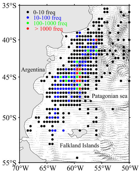
Figure 1.
Spatial distribution of the total frequency of CPUE ≥ 5.
The gray arrows in the figure indicate the ocean currents and their directions, as generated from sea surface velocity data (u: horizontal velocity; v: vertical velocity). The sea surface velocity data were obtained from the Copernicus Marine Environment Monitoring Service (CMEMS).
2.2. Environmental Data
The mesoscale eddy data in this study were derived from the multi-satellite altimeter data fusion provided by the Copernicus Marine Environment Monitoring Service (CMEMS) multi-satellite altimetry merged product (https://marine.copernicus.eu/, accessed on 10 July 2023). The dataset encompasses Absolute Dynamic Topographies (ADT) and sea surface-current velocity data, covering a spatial domain of 50°–70°W and 35°–55°S with a spatial resolution of 1/4° and a temporal resolution of one day. To ensure the continuity and integrity of eddy data, the download time range for eddy data spans from 2012 to 2019.
Based on previous research findings [19,28], three environmental factors—sea surface temperature (SST), temperature at 200 m depth (T200m), and chlorophyll-a concentration (Chl-a) — were selected to analyze the regulatory role of mesoscale eddies on the environment and their impact on the distribution of I. argentinus. Temperature data were sourced from the Global Ocean Physical Ensemble Reanalysis product (https://data.marine.copernicus.eu/product/GLOBAL_MULTIYEAR_PHY_ENS_001_031/description, accessed on 10 July 2023) of CMEMS, while Chl-a data were obtained from the Global Ocean Biogeochemical product (https://data.marine.copernicus.eu/product/GLOBAL_MULTIYEAR_BGC_001_029/description, accessed on 11 July 2023) of CMEMS. All environmental data covered the spatial range of the fisheries data, with spatial and temporal resolutions of 1/4◦ and one day, respectively. Based on temporal sequences and spatial positions, the environmental data corresponding to the fisheries and eddy data were linearly interpolated, yielding environmental data for each fisheries record and daily eddy environmental data for the entire life cycle of each eddy.
2.3. Mesoscale Eddy Data
Employing the Angular Momentum Eddy Detection and Tracking Algorithm (AMEDA) method [29], based on physical parameters and geometric characteristics, mesoscale eddies in the Patagonian region (55°–30°S, 70°–50°W) were identified and tracked from 2012 to 2019. A total of 2262 eddies, comprising 1119 CEs and 1143 AEs, were identified using the Lagrangian eddy-counting method. The average radii of cyclonic and anticyclonic eddies were 41.08 km and 39.15 km, respectively. To investigate eddy characteristics, this study employed the Exclusive Economic Zone (EEZ) boundary as a demarcation. Results indicated that eddies that formed near the coastline and Falkland Islands propagated eastward, while others moved westward uniformly. No significant differences in eddy movement were observed within the study area. The initial positions and trajectory maps of eddies are provided in Supplementary File S1, Figures S1 and S2.
To compare differences in resource abundance and environmental conditions within eddies across their life stages, we normalized the life cycle of each eddy, using the methods of Yang et al. (2022) and Liu et al. (2012), to a continuous value ranging from 0 to 1 [30,31,32]. Based on the stage-like characteristics of eddy parameters within this normalized life cycle, we divided the eddies’ life cycles into four life stages: formation (0–0.1), intensification (0.1–0.3), maturity (0.3–0.8), and decay (0.8–1). Specifically, these stages correspond to rapid growth in eddy radius and rotational velocity, slow growth to peak values, stabilization, and rapid decline, respectively (Figure 2).
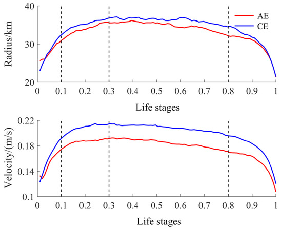
Figure 2.
Time evolution of the normalized radius and rotation velocity of CEs and AEs.
2.3.1. Relationship Between Squid Resource Abundance and Eddy Position
To determine the effect of eddies on squid distribution within the fishing grounds, three indicators—catch, fishing effort, and occurrences of CPUE ≥ 5—were used to represent the abundance of I. argentinus [22,32]. The changes in squid abundance within 2R of CEs and AEs and their relationship to the distance from the eddy center were analyzed. Catch refers to the weight of I. argentinus captured daily at each fishing site and serves as a direct indicator of fishery resource abundance. Effort denotes the input used for fishing and is measured in this study as the number of days. Total occurrence of CPUE refers to the cumulative frequency or number of occurrences where the CPUE value is greater than or equal to 5. This metric helps analyze the concentration and spatial variability of resource distribution.
Due to the varying shape and size of eddies, a normalized eddy-center coordinate system was used to mitigate the impact of eddy size differences [24,30]. In this coordinate system, the normalized radius of fishery eddy is characterized by the equivalent radius of a circle with an area equivalent to that of the eddy. Specifically, the inner eddy area is delineated by 0 to R and the edge area by R to 2R.
Mesoscale eddies have a positive impact on the aggregation of I. argentinus resources. For a detailed comparison of resource abundance within eddies and in external regions, please refer to Supplementary File S1, Table S1. To analyze the distribution of resources within eddies, we constructed a normalized radial-distance grid to represent the daily influence area of each eddy, based on the normalized radius mentioned above. Linear interpolation methods were used based on temporal sequences and spatial positions to match each fisheries data record with the eddies’ tracking data. The occurrences of catch, effort, and CPUE ≥ 5 were projected onto the corresponding normalized grids for each day. We then aggregated the occurrences of catch, effort, and CPUE ≥ 5 within each grid cell to obtain the distribution of resource abundance within the eddies. Additionally, fisheries data within 2R of eddies were selected and the normalized relative distances were divided into 20 intervals of 0.1 times the radius. The total catch, total fishing effort, and total occurrences of CPUE ≥ 5 in each interval were calculated to compare the distribution of I. argentinus inside and outside CEs and AEs. The normalized relative distance was computed as follows:
Here, Z are the zonal and meridional distances from the fishing position to the closest CE or AE center, R represents eddy radius, and D are the normalized zonal and meridional relative distances, respectively. Additionally, a simple in-polygon algorithm was applied to accurately determine whether the fishing position was in the interior of an eddy, as the contours of eddies had been defined as approximate polygons.
To explore the relationship between squid distribution and eddy position at different stages, the relationship between the I. argentinus CPUE at various fishing locations and eddy centers was analyzed using normalized relative distances. The center of gravity of CPUE in both longitudinal and latitudinal directions within the influence range of eddies at different stages were calculated, and these were compared with the average position of eddy centers for all fishery-related eddies. The centroid longitude and latitude of CPUE were calculated using the following formulae:
Here, LONG and LATG are the longitude and latitude center of gravity of the CPUE, respectively; Xi is the longitude of the fishing position; and Yi is the latitude of the fishing position in the eddy life stages.
2.3.2. Environmental Variations Within Eddy Life Stages
To analyze the variations of SST, T200m, and Chl-a within and outside the fishery-related eddies across the life stages, these environmental factors were interpolated daily into each eddy grid using linear interpolation based on temporal sequences and spatial positions. The daily eddy grids were then aggregated according to the eddy life stage and averaged across multiple grids for all life stages, yielding a distribution of average environmental factors within eddies throughout the life cycle. The distribution of environmental characteristics within the study area, as well as the results of the comparative analysis between the internal environment of eddies and the surrounding sea areas, are presented in Supplementary File S1, Figure S3 and Table S2.
2.3.3. Variations in Habitat Suitability Within Eddy Life Stages
A suitability index (SI) and habitat suitability index (HSI) model were used with the arithmetic average method (AMM) to analyze the impacts of eddy evolution on the distribution and abundance of I. argentinus. The calculation methods and results of the model construction with the SI and HSI models are detailed in Supplementary File S2 [19,32,33,34,35,36,37,38]. According to the optimal weighting scheme derived from findings, the environmental factors within the eddy grids were substituted into the SI and HSI models. The SI and HSI distributions at different daily eddy stages were calculated and averaged to determine the proportion of suitable single-factor environmental conditions and suitable habitat areas (SI ≥ 0.6 and HIS ≥ 0.6) within CEs and AEs.
2.4. The Effect of Eddy Evolution on Squid Habitat Suitability, Investigated Using Case Studies
This study selected six eddies (500, 1415, 2240, 1630, 1662, and 1945) with varying lifetimes (88, 36d, 110d, 96d, 110d, 92d) to investigate the effects of eddy evolution on the distribution and habitat suitability of I. argentinus. These eddies encompassed both AEs (eddies 500, 1415, 2240) and CEs (eddy 1630, 1662 1945). Additionally, the eddies were chosen from different geographical locations and included both coastal eddies (eddies 500, 1945) and open-ocean eddies (eddies 1415, 2240, 1630, 1662). Furthermore, the selection included fisheries-related eddies (eddies 500, 1630, 1662) and non-fisheries eddies (eddy 1415, 1945, 2240), ensuring comprehensive coverage of fishing grounds in both nearshore and high-seas areas. These eddies had relatively long lifespans and included a relatively complete HSI variation process from January to April (the formation stage of eddy 1630 and the decay stage of eddy 1662 occurred from May to December; therefore, no HSI values were available for these stages). The average HSI distribution patterns across the different life stages of these six eddies were analyzed, and the average HSI values within each life stage were calculated.
3. Results
3.1. Variations in the Distribution and Abundance of I. argentinus Across Eddy Life Stages
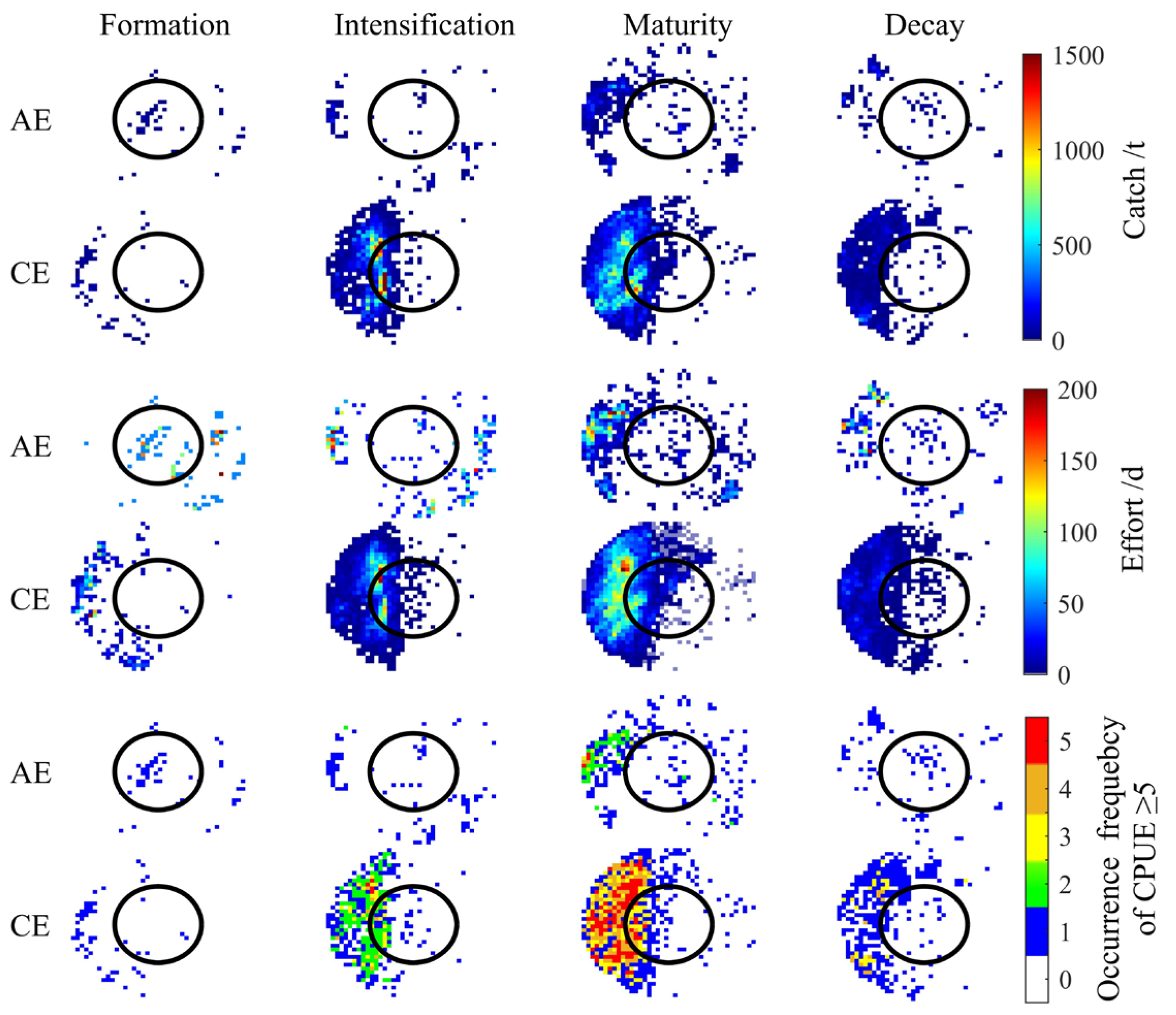
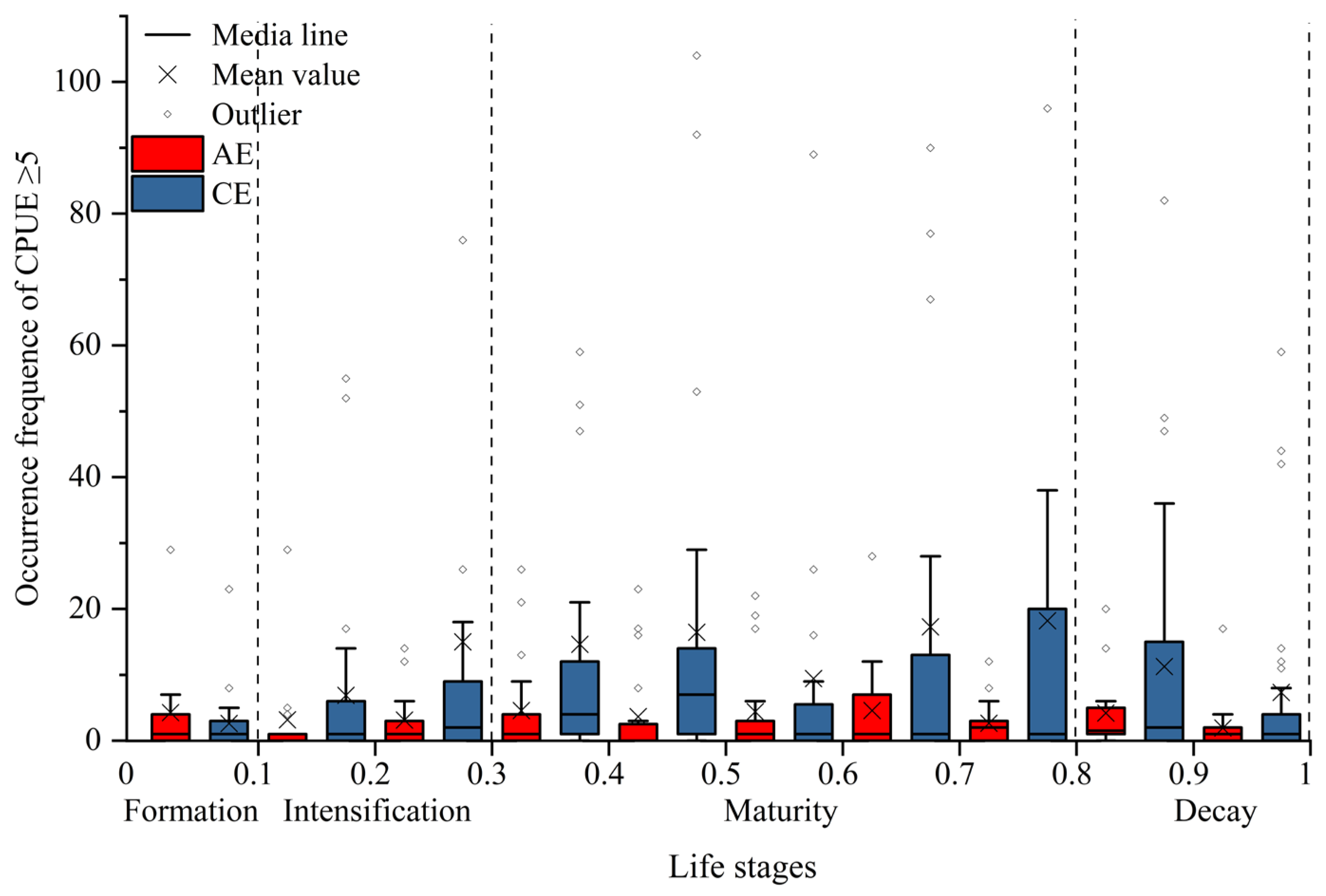
CEs and AEs significantly influenced the spatial distribution of I. argentinus resources during different eddy stages, with the most pronounced effects occurring during the maturation stage. As shown in Figure 3, squid abundance in both CEs and AEs increased and then decreased with eddy evolution, reaching a peak during the maturation stage. Spatially, squid were mainly distributed in the peripheral region (from R to 2R) to the northwest and southeast of AEs, while in CEs, squid were concentrated in the inner edge (R) to the west of the eddy and in the outer region (from R to 2R). As shown in Figure 4, both CEs and AEs exhibited significantly higher CPUE values during the maturation stage. The average occurrences of CPUE ≥ 5 were higher in CEs than in AEs during the intensification, maturation, and decay stages, although not during the formation stage. To clearly elucidate the impact of eddy type and life stages on resource abundance, we quantified fishery-related eddies by life stage and calculated the proportion of eddies with CPUE ≥ 5. Detailed data are in Supplementary Materials File S1;Table S3.
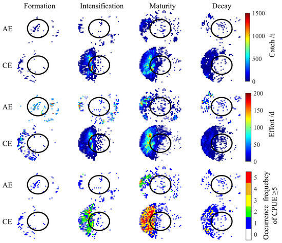
Figure 3.
Spatial distribution of cumulative catch, cumulative fishing effort, and total occurrences of CPUE ≥ 5 across eddy life stages.
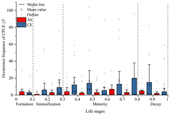
Figure 4.
Variation in the occurrences of CPUE ≥ 5 across eddy life stages.
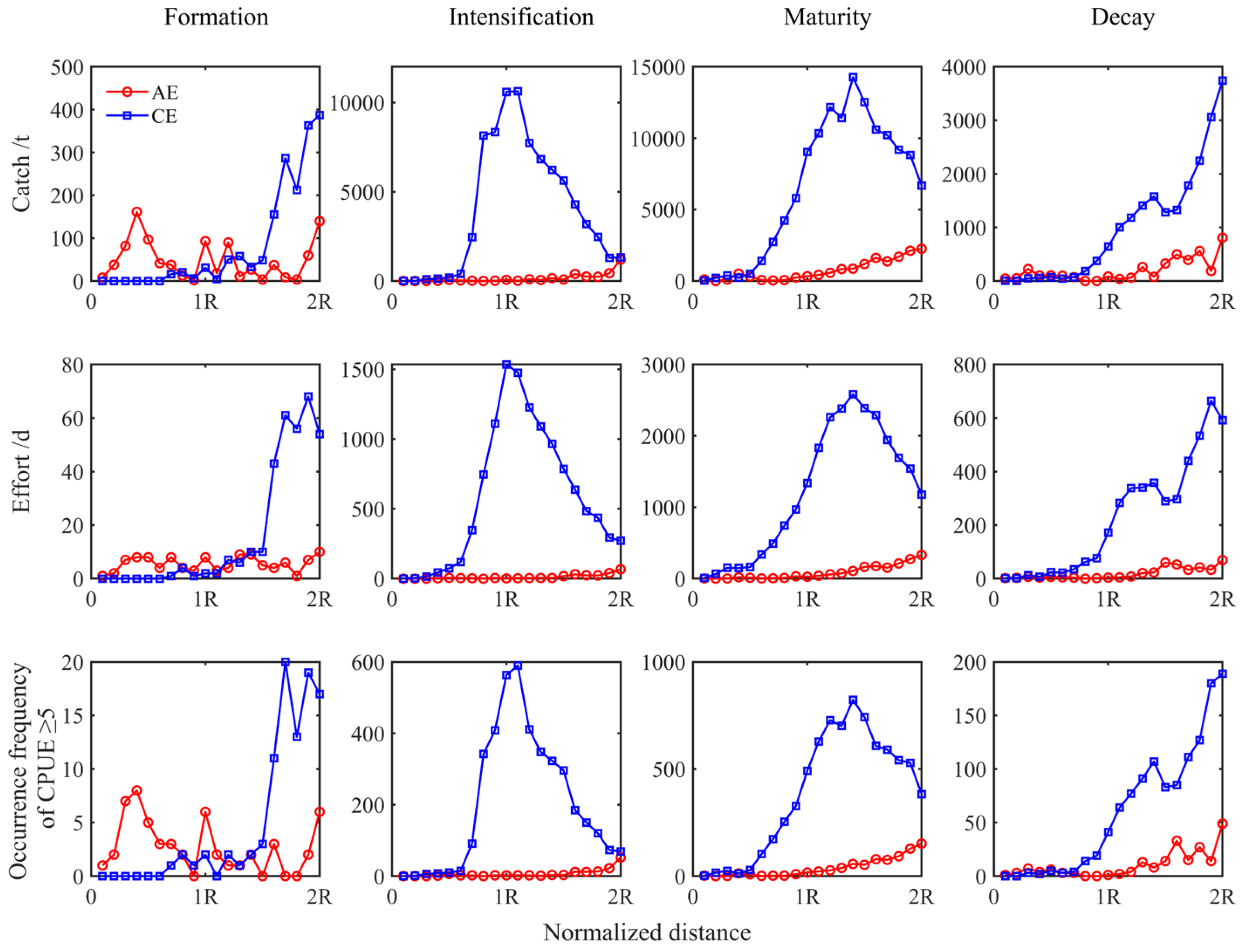
Variations in the abundance of I. argentinus, as indicated by the cumulative catch, cumulative fishing effort, and total occurrences of CPUE ≥ 5, from the eddy core to the eddy edge of CEs and AEs during evolution, were analyzed (Figure 5). Squid abundance within two radius intervals was greater in CEs than in AEs, except in the formation stage. In CEs, squid abundance increased and then decreased with increasing distance from the eddy center during the maturation phase and gradually increased during decay. In AEs, squid abundance fluctuated during eddy formation, with a distinctly greater abundance within AEs. From eddy intensification to decay, the trend in squid abundance was consistent, with total catch, total fishing effort, and the frequency of CPUE ≥ 5 gradually increasing with increasing distance from the eddy center and reaching a peak at the peripheral edge of AEs.
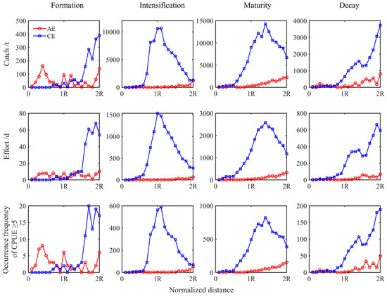
Figure 5.
The relationship between cumulative catch, cumulative fishing effort, and the occurrences of CPUE ≥ 5 with the distance from the eddy center across eddy life stages.
3.2. Spatial Relationship Between Eddy Centers and CPUE Center of Gravity
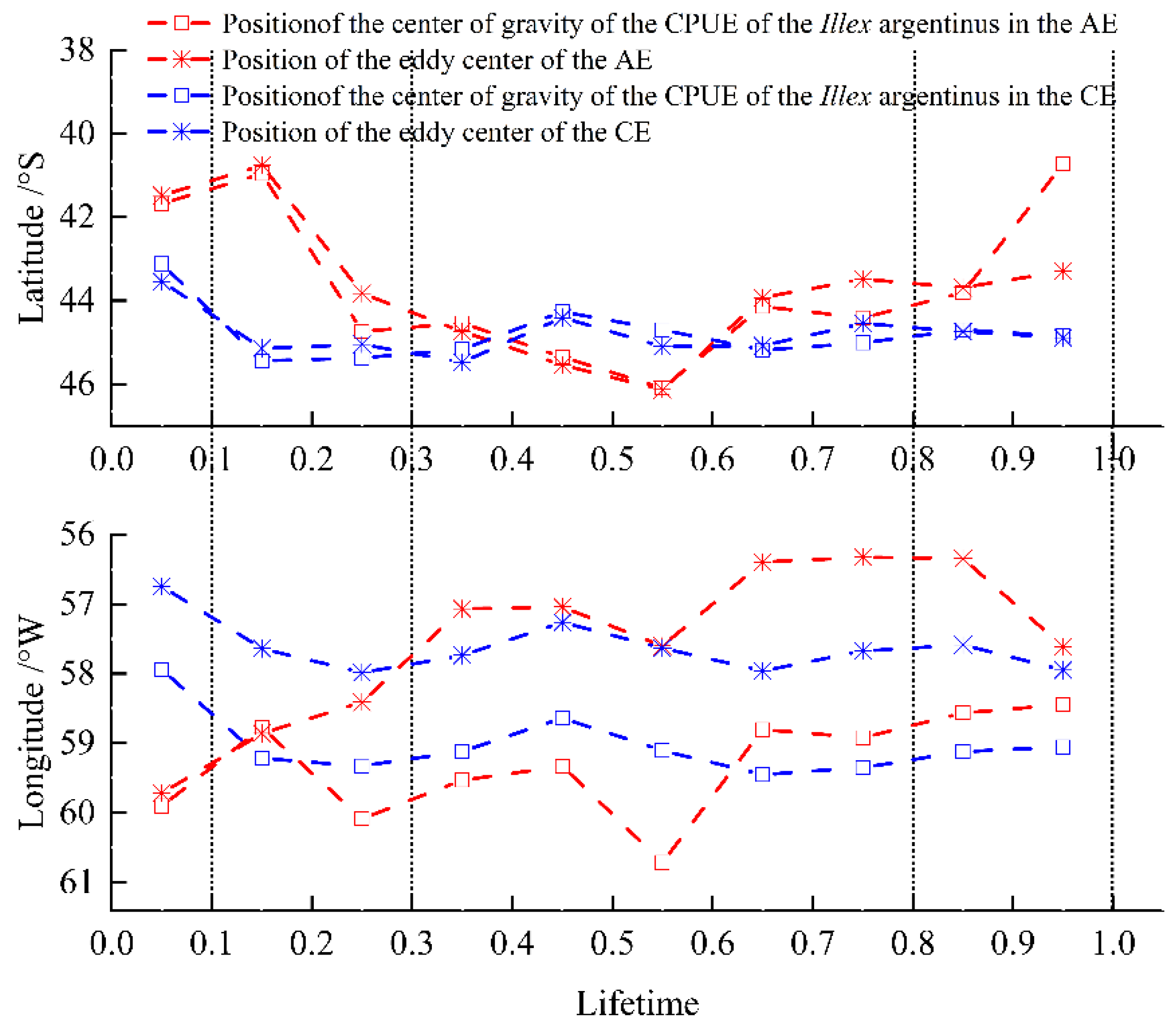
During the life cycles of all fishery eddies, the CPUE center of gravity of I. Argentinus within the eddies followed the changing location of the eddy center (Figure 6). Longitudinally, both the eddy center and the CPUE center of gravity of AEs exhibited eastward movement, while those of CEs moved westward. After initial convergent motion during eddy intensification, the eddy center and the CPUE center of gravity of AEs maintained movement in a consistent direction, with a pronounced eastward trend in the movement of the eddy centers. The CPUE center of gravity was consistently west of the eddy center in both CEs and AEs in the longitudinal direction. Latitudinally, the overall movements of the eddy centers and the CPUE center of gravity of AEs trended southward and northward, respectively. These trends were aligned from eddy formation to maturation, but during decay, they diverged. In contrast, the eddy centers and the CPUE center of gravity of CEs shared a consistent southward trend in their movement. The center of gravity of CPUE is almost aligned with the vortex centers of CE and AE in the latitudinal direction.
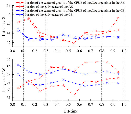
Figure 6.
Variation in the locations of the eddy center and the CPUE center of gravity of I. argentinus across eddy life stages.
3.3. Spatial Distribution Patterns of SST, T200m, and Chl-a Within Eddy Life Stages
Figure 7 examines the spatial distributions of the selected environmental parameters within eddies during their various life stages. Both SST and T200m were higher in the AEs across the eddy life cycle than in CEs. In contrast, Chl-a was higher in CEs from eddy formation to maturation and higher in AEs during eddy decay. Within CEs, SST initially decreased and then increased, with the lowest temperatures occurring during the intensification stage. In contrast, T200m initially increased, then decreased, and then subsequently increased, with the lowest temperatures being recorded during the mature stage. Spatially, both SST and T200m showed lower temperatures on the left periphery of the eddy compared to the interior and the right peripheral regions. Chl-a was higher on the right peripheral region of CEs during the formation stage, with no significant differences observed across the other life stages. In AEs, SST and T200m initially decreased and subsequently increased, with the highest temperatures occurring during the formation stage and the lowest occurring during maturation. Chl-a concentration gradually increased with AE evolution, reaching a peak during eddy decay. SST was lower on the southern periphery; T200m was lower on the western periphery; and Chl-a was higher on the northwest and southeast sides of AEs.
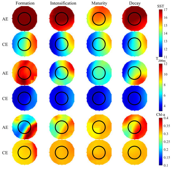
Figure 7.
Spatial distribution of SST, T200m, and Chl-a within eddies across their life cycles.
3.4. Variations in SI and HSI Across Eddy Life Stages
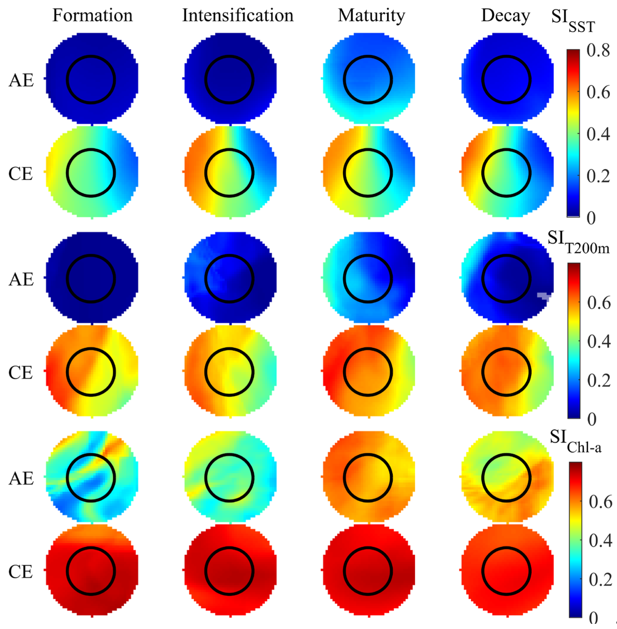
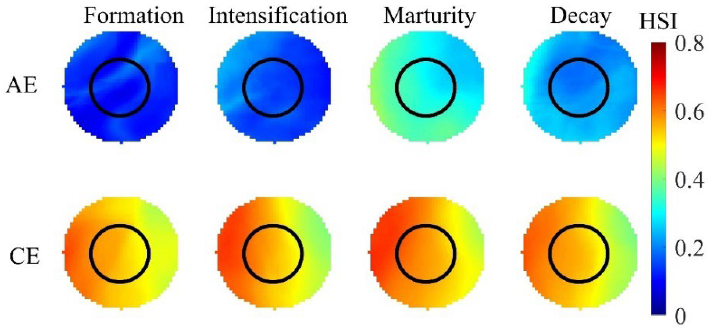
The average distribution patterns of SI and HSI for the three selected environmental factors during eddy evolution are presented in Figure 8 and Figure 9. Both SI and HSI within AEs exhibited a gradual increase from eddy formation to maturation, which was followed by a decline during the decay stage. The optimal SI and HSI values were attained during the intensification and maturation stages of AEs, respectively. Within these eddies, higher SISST, SIT200m, and SIChl-a values were localized in the southern, western peripheral, and northeastern regions, respectively. Higher HSI values were primarily distributed in the northwestern region of the eddy during both the intensification and the decay stages and in the northwestern to southeastern peripheral areas during maturation. Additionally, the suitability of different environmental factors varied across the life stages of CEs. SISST, SIT200m, and HSI all demonstrated an initial increase followed by a decrease, with SISST reaching its peak during CE intensification and SIT200m and HSI peaking during eddy maturation. In contrast, SIChl-a exhibited minimal variation across CE life stages. The SISST, SIT200m, and HSI values in CEs were highest in the western and lower in the eastern regions, with high SIChl-a present throughout the entire influence range of the CEs.

Figure 8.
Distribution of suitability indices (SI) across eddy life stages.

Figure 9.
Distribution of habitat suitability indices (HSI) across eddy life stages.
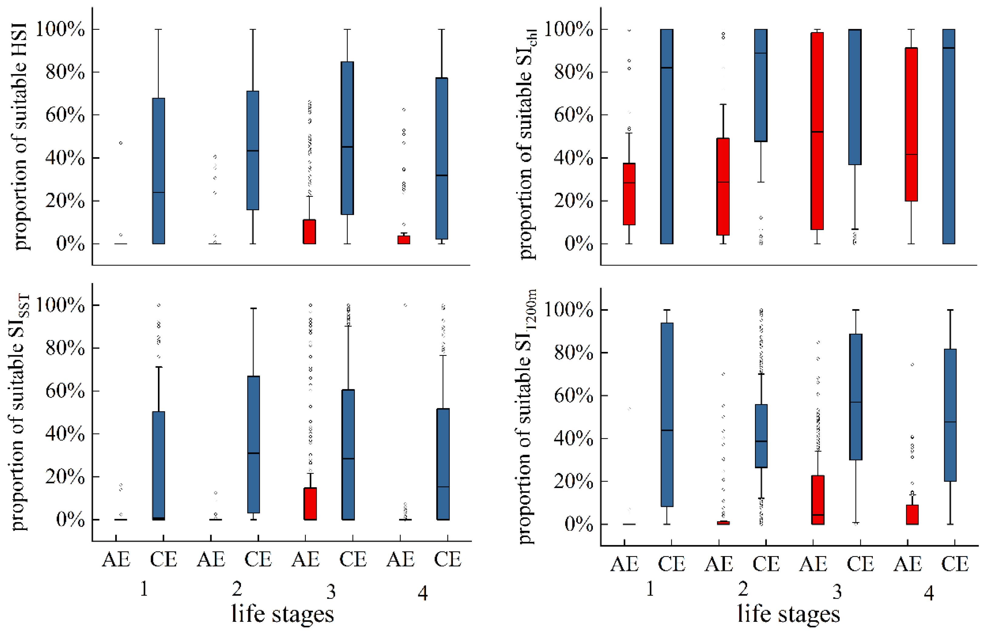
Figure 10 illustrates the variation in the proportion of suitable SIs (SI ≥ 0.6) and suitable HSIs (HSI ≥ 0.6) across eddy evolution. Apart from SIChl-a, the proportions of suitable SISST, SIT200m, and HSI within AEs were relatively low, with a gradual increase from eddy formation to maturation, and significantly decreased during decay. In CEs, the proportions of suitable SISST, SIT200m, SIChl-a, and HSI were comparatively higher across all life stages. The proportions of suitable SISST and HSI gradually increased throughout eddy evolution but decreased during eddy decay. Suitable SIT200m and SIChl-a were detected in distinctly higher proportions during CE formation.
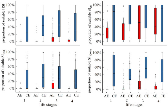
Figure 10.
Proportion of suitable SISST, SIT200m, SIChl-a, and HSI across eddy life stages.
3.5. Variations of HSI Across the Life Cycle of Six Eddies
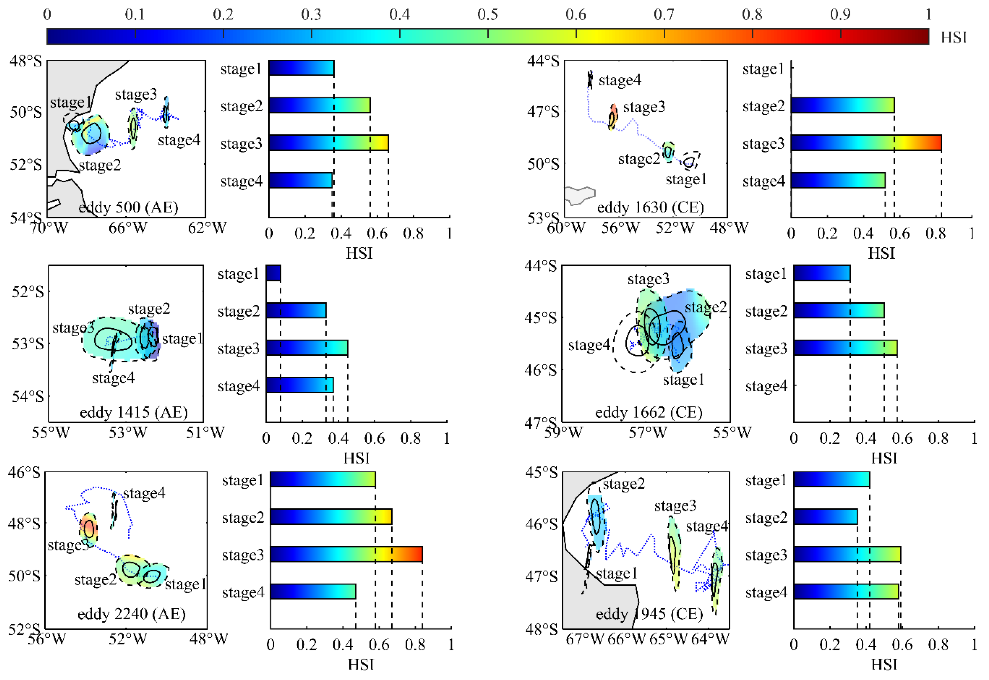
Figure 11 presents the evolutionary trajectories of different types of eddies (AE and CE) across distinct geographical regions (coastal and open seas), including fishery-related eddies (eddies 500, 1630, 1662) and non-fishery eddies (eddies 1415, 1945, 2240). It also illustrates the spatial distribution of HSI within these eddies during their various life cycles and provides statistical summaries of the average HSI levels within the eddies (Figure 11). It is evident that the HSI values within each life stage of the eddies in all cases gradually increase and then decrease as the eddies evolve. The peak HSI levels are consistently reached during the mature stage, aligning with the average HSI distribution results within the eddies, as shown in Figure 9.
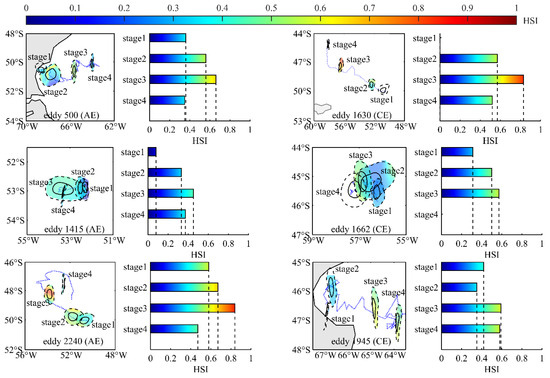
Figure 11.
Eddy case studies: spatial distribution of average HSI values across eddy life stages and bar charts illustrating the average HSI within each stage.
4. Discussion
4.1. Environmental Changes Across Eddy Life Stages
This study reveals the impact of CEs and AEs across eddy evolution on the water temperature structure within Patagonian waters. The results indicate that CEs regulate the hydrological structure of localized seaareas through internal upwelling processes that result in cooler temperatures within the CEs compared to the surrounding waters, while AEs are warmer due to internal downwelling. Regions of low SST and T200m were concentrated in the western region of CEs and the southern region of AEs, aligning with higher temperatures in the north and lower temperatures in the south observed in Patagonian ocean waters [19,39]. In this study, T200m in both CEs and AEs and SST in AEs reached their lowest values during eddy maturation, suggesting that dynamic structural changes within the eddy are most pronounced during this stage. The maximum increase in temperature change induced by intense vertical stratification during the maturation of eddies likely promotes the mixing and transport of heat from the ocean surface downward, achieving maximum cooling within the eddy. It has been documented that the temperature perturbations induced by eddies near the Antarctic Circumpolar Current (ACC) are the strongest where dynamic processes are prominent and seawater temperature variations are significantly influenced by water entrainment caused by the cross-frontal displacement of eddies [40]. There are distinct differences in how CEs and AEs affect Chl-a concentrations across the various life stages. This study found that from the formation to the maturation stage, Chl-a concentrations were slightly higher in CEs than in AEs and were more uniformly distributed throughout eddy evolution. In contrast, AEs had a distinct edge-enhancement phenomenon. This is consistent with previous findings that productivity is higher in CEs compared to AEs [8,40,41]. The distribution of Chl-a both inside and outside mesoscale eddies is regulated by different mechanisms; within the inner region within one radius, Chl-a distribution is primarily influenced by dynamic processes such as eddy pumping, eddy trapping, and eddy-Ekman pumping, whereas in the outer region from one to two radii, Chl-a distribution is mainly controlled by eddy edge advection and frontal dynamics [42,43]. Notably, both I. argentinus and juvenile loggerhead sea turtles (Caretta caretta) prefer low-chlorophyll regions in the Brazil-Malvinas Confluence (BMC). Gaube et al. (2017) attributed this to AEs causing downwelling, which raises sea surface temperatures, inhibits phytoplankton growth, and facilitates the formation of low Chl-a zones. These zones, with higher temperatures and potentially concentrated prey resources, offer advantageous conditions for marine species like loggerhead sea turtles [27].
4.2. Characteristics of I. argentinus Resources Across Eddy Life Stages
This study revealed that there was a higher abundance of I. argentinus in CEs, which provide more suitable habitats for this species in Patagonian waters. The abundance of I. argentinus in both CEs and AEs initially increased and then decreased throughout eddy evolution, with the highest abundance during maturation. Additionally, the distribution of I. argentinus was denser in the edge areas of both CEs and AEs. This may be attributed to the biological aggregation effect at the eddy edges, the frontal structure, and the upwelling and downwelling, which collectively enhance productivity and species diversity in the edge areas [44,45,46], providing more feeding opportunities for I. argentinus. Figure 5 shows that the abundance varies with distance from eddy centers, peaking near R = 1 for CE and R = 2 for AE. R=1 delineates the eddy’s internal region from its ecological influence, while R = 2 marks the eddy’s influence boundary [30]. These zones are characterized by active physical, ecological, and biogeochemical processes. At R = 1, a high geostrophic-to-translational velocity ratio (U/c > 1) [6] and maximum rotational velocity enhance resource aggregation and material exchange, increasing I. argentinus abundance due to physical effects and prey concentration. Conversely, gentle horizontal velocities at R = 2 coincide with optimal environmental conditions for I. argentinus in the eddy boundary (from R to 2R), as shown in Figure 7, suggesting active habitat selection by I. argentinus.
In the Patagonian sea, CEs generally exhibit a westward and southward propagation trend, while AEs tend to move eastward and northward (Figure 6). During their movement, CEs can entrain nutrient-rich waters from the northward-flowing Falkland Current and high-productivity coastal waters on their western side, significantly enhancing the abundance within the eddy. In contrast, AEs propagate through more oligotrophic waters influenced by the Brazil Current and open-ocean regions, making it difficult for them to replenish nutrients effectively. This may be one reason why the abundance of I. argentinus is higher in CEs than in AEs. Notably, the center of CPUE gravity is located farther to the west compared to the eddy center in the longitudinal direction (Figure 6). This phenomenon is considered reasonable. According to the results in Figure 3, the abundance of I. argentinus in CEs is highly concentrated within the range from 0 to R on the western side of the eddy, while the resources in AEs are mainly aggregated within the range from R to 2R on the northwest side of the eddy. These findings not only align with previous analyses but also further confirm that the resource gravity center is indeed located to the west of the eddy center, thereby strengthening our argument.
Mesoscale eddies, as complex marine dynamic processes, play a significant role in regulating ocean biogeochemical cycles and climate change in the southwest Atlantic Ocean [47,48]. This study posits that during eddy evolution in Patagonian waters, eddy structure and intensity are relatively weak in the initial formation stage [49], having a minor impact on the surrounding sea environment and thus not significantly impacting catch. Intensity increases with eddy evolution, potentially triggering strong upwelling or downwelling, bringing deep nutrients to the surface or surface nutrients to the deep, providing a rich food source, and attracting large aggregations of fish near the eddy [50]. Moreover, eddy intensification may gradually change the surrounding seawater temperature and salinity and other environmental factors, further affecting the distribution of fish and thus of catch, which usually increases during this eddy life stage. When the eddy reaches maturation, its structure and intensity are relatively stable [51,52], providing a suitable and stable habitat for Argentine shortfin squid, which in turn promotes large aggregations to form fishing grounds within the eddy during this phase. During eddy decay, its intensity and structure gradually weaken, and it eventually disappears. This results in a decreased impact on the surrounding seawater, which causes the distribution of nutrients and other environmental factors to return to normal, causing a decrease in catch within the eddy [8,53].
4.3. The Impact of Eddy Evolution on SI and HSI
The HSI model is one of the most important tools for species management and fishing-ground prediction and has been widely used to evaluate the habitat and fishing-ground distributions of oceanic cephalopods such as the Humboldt squid Dosidicus gigas [54] and S. oualaniensis [55]. In this study, the impact of CE and AE evolution on the distribution and abundance of I. argentinus showed significant differences related to the squid’s varying mechanisms of response to a changing environment within the eddy. During eddy formation, a higher abundance of I. argentinus corresponded to lower temperatures and Chl-a concentrations. As the eddy evolved, high SI and HSI values were mainly distributed in low-temperature, high-Chl-a regions from intensification to decay. The environmental changes that occur during eddy evolution form a more suitable habitat for I. argentinus. SI, HSI, and squid abundance in both CEs and AEs gradually increased and reached a peak during the formation, intensification, and maturation stages, decreasing during eddy decay. The changes in SI and HSI directly affected the spatial distribution and abundance of I. argentinus.
To validate prior perspectives, this study analyzed six mesoscale eddies of various types in the Patagonian Sea. The objective was to assess how eddy evolution influences the resource distribution and habitat suitability (HSI) of I. argentinus, validating trends observed in resource abundance and HSI changes across eddy life stages (Figure 3 and Figure 9). During the formation stage, all eddies exhibited low HSI for I. argentinus. Conversely, HSI peaked during the mature stage, aligning with the observed trends of initially increasing and then decreasing resource abundance and HSI across different eddy life stages. This confirms that the squid’s distribution and abundance are significantly regulated by mesoscale eddy evolution, with the mature stage having the most significant impact on resource abundance. Importantly, these six eddies, encompassing fishery-related, non-fishery, and geographically distinct types, shared the common trait of HSI increasing and then decreasing around the mature stage. This suggests it may be a ubiquitous characteristic of eddies in this region.
Illex argentinus exhibits pronounced seasonal variation in water-layer habitat selection, preferring deeper and colder layers during winter (from June to August) and warmer, shallower layers during summer (from December to February) [19]. In this study, the increase in the SST during CE maturation resulted in an expansion of less suitable habitat conditions within these eddies. However, this adverse effect is counterbalanced by the high proportion of suitable SST and Chl-a indices within CEs, resulting in a continued increase in the distribution of suitable habitats from formation to maturation. During CE and AE decay, the proportion of suitable SI and HSI areas and squid abundance decrease. However, the decline does not bring the values back to those observed at eddy formation (Figure 3). Multiple factors contribute to this phenomenon. During the decay of mesoscale eddies, internal water movement and vertical exchange weaken, yet prior to this, eddies enrich the upper ocean with nutrients from deep water via Ekman pumping, maintaining high nutrient levels. Even in decay, eddies continue to mix water masses of varying depths, temperatures, and nutrient contents until dissipation, providing favorable conditions for Argentine shortfin squid. Additionally, during decay, the gradual disappearance of "ecological conduits" (facilitating fish downward foraging) and "ecological barriers" (hindering downward movement) [8] alters fish behavior. Deep-diving predators like tuna become more active in upper layers, increasing their susceptibility to capture, while fish constrained by ecological barriers gain expanded foraging and movement ranges, boosting fishing yields.
5. Conclusions
In summary, the study aims to investigate how environmental changes induced by eddies influence the spatial and temporal abundance of I. argentinus and to elucidate the mechanisms underlying these impacts. The mature stage of eddy evolution exhibits the most pronounced influence on the abundance and distribution of I. argentinus in Patagonian waters. During this stage, habitat suitability and resource abundance reach their peak. There is a higher abundance of I. argentinus and greater habitat suitability within CEs compared to AEs. Specifically, squid are primarily concentrated in the peripheral area on the west side of CEs and in the peripheral regions to the northwest and southeast of AEs. Notably, low-temperature environments concurrently enhance the SI and HSI in both CEs and AEs.
This study not only enhances our understanding of how eddy evolution influences the distribution of fishery resources but also provides a scientific basis for optimizing fishing strategies and implementing sustainable resource management. Although this study has made significant strides in revealing the impacts of eddies on squid abundance and distribution, it is constrained by its reliance on remote sensing and fishing data, lacking in situ observational data to validate the ecological processes that occur within the eddies. Furthermore, this study did not fully account for other potential influencing factors such as ocean acidification and climate change. Therefore, future research should integrate in situ observations to further explore the complex impacts of eddies and other environmental factors on the abundance and distribution of I. argentinus and the resulting ecosystem effects. This approach will help address the challenges posed by global changes and promote long-term sustainable use and conservation of fishery resources.
Supplementary Materials
The following supporting information can be downloaded at: https://www.mdpi.com/article/10.3390/jmse13020288/s1, Figure S1: The spatial distribution of the generation and dissipation points of all vortices within and outside the EEZ from 2013 to 2019.; Figure S2: The absolute motion trajectories of all cyclonic and anticyclonic eddies within and outside the EEZ from 2013 to 2019.; Figure S3: Spatial distribution of average SST, T200m, and Chl-a in the Patagonian Sea.; Table S1: Statistics of total catch and total fishing effort in eddies and non-eddy areas; Table S2: Environmental average values of eddies at different life stages and the overall study area in the Patagonian Sea. The modeling process of habitat suitability index (HSI) model can be found in Supplementary File S2.
Author Contributions
Conceptualization, L.Z. and W.Y.; methodology, L.Z., P.Z. and W.Y.; soft-ware, L.Z. and W.Y.; validation, L.Z. and W.Y.; formal analysis, L.Z. and W.Y.; investigation, L.Z. and P.Z.; resources, W.Y.; data curation, L.Z.; writing—original draft preparation, L.Z. and W.Y; writing—review and editing, W.Y.; visualization, L.Z.; supervision, W.Y.; project administration, Z.Z. and W.Y; funding acquisition, Z.Z. and W.Y. All authors have read and agreed to the published version of the manuscript.
Funding
This study was financially supported by the Natural Science Foundation of Shanghai (23ZR1427100), the National Key R&D Program of China (2023YFD0901405), and the Shanghai talent development funding (2021078).
Institutional Review Board Statement
Not applicable.
Informed Consent Statement
Not applicable.
Data Availability Statement
Data would be made available upon request from the corresponding author.
Conflicts of Interest
The authors declare that they have no known competing financial interests or personal relationships that could have appeared to influence the work reported in this paper.
References
- Early, J.J.; Samelson, R.M.; Chelton, D.B. The evolution and propagation of quasigeostrophic ocean eddies. J. Phys. Oceanogr. 2011, 41, 1535–1555. [Google Scholar] [CrossRef]
- Zhang, Z.; Tian, J.; Qiu, B.; Zhao, W.; Chang, P.; Wu, D.; Wan, X. Observed 3D structure, generation, and dissipation of oceanic mesoscale eddies in the South China Sea. Sci. Rep. 2016, 6, 24349. [Google Scholar] [CrossRef] [PubMed]
- Renault, L.; Masson, S.; Oerder, V.; Jullien, S.; Colas, F. Disentangling the mesoscale ocean-atmosphere interactions. J. Geophys. Res. Ocean. 2019, 124, 2164–2178. [Google Scholar] [CrossRef]
- Chelton, D.B.; Schlax, M.G.; Samelson, R.M. Global observations of nonlinear mesoscale eddies. Prog. Oceanogr. 2011, 91, 167–216. [Google Scholar] [CrossRef]
- Garcia, C.A.E.; Sarma, Y.V.B.; Mata, M.M.; Garcia, V.M.T. Chlorophyll variability and eddies in the Brazil–Malvinas Confluence region. Deep Sea Res. Part II Top. Stud. Oceanogr. 2004, 51, 159–172. [Google Scholar] [CrossRef]
- Zhang, Y.C.; Wang, N.; Zhou, L.; Liu, K.F.; Wang, H.D. The surface and three-dimensional characteristics of mesoscale eddies: A review. Adv. Earth Sci. 2020, 35, 568–580. [Google Scholar] [CrossRef]
- Cabrera, M.; Santini, M.; Lima, L.; Carvalho, J.; Rosa, E.; Rodrigue, C.; Pezzi, L. The southwestern Atlantic Ocean mesoscale eddies: A review of their role in the air-sea interaction processes. J. Mar. Syst. 2022, 235, 103785. [Google Scholar] [CrossRef]
- Xing, Q.W.; Yu, H.Q.; Wang, H.; Ito, S.; Chai, F. Mesoscale eddies modulate the dynamics of human fishing activities in the global midlatitude ocean. Fish Fish. 2023, 24, 527–543. [Google Scholar] [CrossRef]
- Zhang, Y.C. The Effects of Mesoscale Eddies on the Abundance and Distribution of Neon Flyings Quid in the Northwest Pacific Ocean. Master’s Thesis, Shanghai Ocean University, Shanghai, China, 2023. [Google Scholar] [CrossRef]
- Hsu, A.C.; Boustany, A.M.; Roberts, J.J.; Chang, J.H.; Halpin, P.N. Tuna and swordfish catch in the US northwest Atlantic longline fishery in relation to mesoscale eddies. Fish. Oceanogr. 2015, 24, 508–520. [Google Scholar] [CrossRef]
- Gaube, P.; Braun, C.D.; Lawson, G.L.; McGillicuddy Jr, D.J.; Penna, A.D.; Skoma, G.B.; Fischer, C.; Thorrold, S.R. Mesoscale eddies influence the movements of mature female white sharks in the Gulf Stream and Sargasso Sea. Sci. Rep. 2018, 8, 7363. [Google Scholar] [CrossRef]
- Mikaelyan, A.S.; Zatsepin, A.G.; Kubryakov, A.A.; Podymov, O.I.; Mosharov, S.A.; Pautov, L.A.; Fedorov, A.V.; Ocherednik, O.A. Case where a mesoscale cyclonic eddy suppresses primary production: A Stratification-Lock hypothesis. Prog. Oceanogr. 2023, 212, 102984. [Google Scholar] [CrossRef]
- Zhang, Z.S.; Xie, L.L.; Li, J.Y.; Li, Q. Comparative analysis of mesoscale eddy evolution during life cycle in marginal seaand open ocean: South China Sea and Kuroshio Extension. J. Trop. Oceanogr. 2023, 42, 63–76. [Google Scholar] [CrossRef]
- Hoerstmann, C.; Aguiar-González, B.; Barrillon, S.; Bastos, C.C.; Grosso, O.; Pérez-Hernández, M.D.; Doglioli, A.M.; Petrenko, A.A.; Carracedo, L.I.; Benavides, M. Nitrogen fixation in the North Atlantic supported by Gulf Stream eddy-borne diazotrophs. Nat. Geosci. 2024, 17, 1141–1147. [Google Scholar] [CrossRef]
- Wu, J.Y.; Chen, X.J.; Fang, X.N. Characteristics of mesoscale eddy in the Eastern Equatorial Pacific Ocean. J. Shanghai Ocean Univ. 2024, 33, 776–785. [Google Scholar] [CrossRef]
- Guo, M.X.; Chai, F.; Xiu, P.; Li, S.Y.; Rao, S. Impacts of mesoscale eddies in the South China Sea on biogeochemical cycles. Ocean Dyn. 2015, 65, 1335–1352. [Google Scholar] [CrossRef]
- Ma, J.Z.; Shi, G.H.; Zhou, T.; Zhen, J.; Yu, C.G.; Cai, X.T. Fishery Biological Properties of Argentine Shortfin Squid in the High Sea of Southwest Atlantic Ocean in 2015. J. Zhejiang Ocean Univ. (Nat. Sci.) 2017, 36, 458–464. [Google Scholar] [CrossRef]
- De la Chesnais, T.; Fulton, E.A.; Tracey, S.R.; Pecl, G.T. The ecological role of cephalopods and their representation in ecosystem models. Rev. Fish Biol. Fish. 2019, 29, 313–334. [Google Scholar] [CrossRef]
- Liu, H.W.; Yu, W.; Chen, X.J.; Zhu, W.B. Construction of habitat suitability index model for Argentine shorfin squid Illex argentinus based on vertical water temperature at different depths. J. Dalian Ocean Univ. 2021, 36, 1035–1043. [Google Scholar] [CrossRef]
- Hou, Q.L.; Chen, X.J.; Wang, J.T. Study on spatio-temporal distribution of Illex argentinus in southwest Atlantic Ocean. Mar. Sci. 2019, 43, 103–109. [Google Scholar] [CrossRef]
- Mason, E.; Pascual, A.; Gaube, P.; Ruiz, S.; Pelegrí, J.L.; Delepoulle, A. Subregional characterization of mesoscale eddies across the Brazil-Malvinas Confluence. J. Geophys. Res. Ocean. 2017, 122, 3329–3357. [Google Scholar] [CrossRef]
- Chiu, T.Y.; Chiu, T.S.; Chen, C.S. Movement patterns determine the availability of Argentine shortfin squid Illex argentinus to fisheries. Fish. Res. 2017, 193, 71–80. [Google Scholar] [CrossRef]
- Liu, H.W.; Yu, W.; Chen, X.J.; Wang, J.T.; Zhang, Z. Influence of Antarctic sea ice variation on abundance and spatial distribution of Argentine shortfin squid Illex argentinus in the southwest Atlantic Ocean. J. Fish. China 2021, 45, 187–199. [Google Scholar] [CrossRef]
- Gaube, P.; Barceló, C.; McGillicuddy, D., Jr.; Doming, A.; Miller, P.; Giffoni, B.; Marcovaldi, N.; Swimmer, Y. The use of mesoscale eddies by juvenile loggerhead sea turtles (Caretta caretta) in the southwestern Atlantic. PLoS ONE 2017, 12, e0172839. [Google Scholar] [CrossRef]
- Lin, D.M. Spawning Strategy of Argentine Shortfin Squid, Illex argentinus (Cephalopoda: Ommastrephidae) in the Southwest Atlantic. Ph.D. Thesis, Shanghai Ocean University, Shanghai, China, 2015. [Google Scholar]
- Liu, Y.; Dong, C.; Guan, Y.; Chen, D.; McWilliams, J.; Nencioli, F. Eddy analysis in the subtropical zonal band of the north Pacific Ocean. Deep Sea Res. Part I Oceanogr. Res. Pap. 2012, 68, 54–67. [Google Scholar] [CrossRef]
- Xu, G.; Dong, C.; Liu, Y.; Gaube, P.; Yang, J. Chlorophyll rings around ocean eddies in the north pacific. Sci. Rep. 2019, 9, 2056. [Google Scholar] [CrossRef]
- Alberto, M.T.; Saraceno, M.; Ivanovic, M.; Acha, E.M. Habitat of Argentine squid (Illex argentinus) paralarvae in the southwestern Atlantic. Mar. Ecol. Prog. Ser. 2022, 688, 69–82. [Google Scholar] [CrossRef]
- Le Vu, B.; Stegner, A.; Arsouze, T. Angular momentum eddy detection and tracking algorithm (AMEDA) and its application to coastal eddy formation. J. Atmos. Ocean. Technol. 2018, 35, 739–762. [Google Scholar] [CrossRef]
- Zhou, K.B.; Benitez-Nelson, C.R.; Huang, J.; Xiu, P.; Sun, Z.Y.; Dai, M.H. Cyclonic eddies modulate temporal and spatial decoupling of particulate carbon, nitrogen, and biogenic silica export in the North Pacific Subtropical Gyre. Limnol. Oceanogr. 2021, 66, 3508–3522. [Google Scholar] [CrossRef]
- Yang, X.; Zhang, Y.C.; Xia, C.S.; Dong, C.M.; Hu, N.; Wang, H.D. Spatiotemporal variations of mesoscale eddies in the Japan Sea. Haiyang Xuebao 2022, 44, 22–36. [Google Scholar]
- Arostegui, M.C.; Gaube, P.; Woodworth-Jefcoats, P.A.; Kobayashi, D.R.; Braun, C.D. Anticyclonic eddies aggregate pelagic predators in a subtropical gyre. Nature 2022, 609, 535–540. [Google Scholar] [CrossRef]
- Tian, S.Q.; Chen, X.J.; Chen, Y.; Xu, L.X.; Dai, X.J. Evaluating habitat suitability indices derived from CPUE and fishing effort data for Ommatrephes bratramii in the northwestern Pacific Ocean. Fish. Res. 2009, 95, 181–188. [Google Scholar] [CrossRef]
- Wen, J.; Lu, X.Y.; Chen, X.J.; Yu, W. Predicting the habitat hot spots of winter-spring cohort of Ommastrephes bartramii in the northwest Pacific Ocean based on the sea surface temperature and photosynthetically active radiation. J. Shanghai Ocean Univ. 2019, 28, 456–463. [Google Scholar] [CrossRef]
- Lei, L.; Wang, J.T.; Chen, X.J.; Lu, J. Standardizing CPUE of Ommastrephes bartramii in the Northwest Pacific Ocean based on environmental factors of habitat. Hai Yang Xue Bao 2019, 41, 134–141. [Google Scholar] [CrossRef]
- Guan, W.J.; Tian, S.Q.; Wang, X.F.; Zhu, J.F.; Chen, X.J. A review of methods and model selection for standardizing CPUE. J. Fish. Sci. China 2014, 852–862. [Google Scholar]
- Yu, W.; Chen, X.; Zhang, Y. Seasonal habitat patterns of jumbo flying squid Dosidicus gigas off Peruvian waters. J. Mar. Systems 2019, 194, 41–51. [Google Scholar] [CrossRef]
- Gong, C.X.; Chen, X.J.; Gao, F.; Guan, W.J.; Lei, L. Review on habitat suitability index in fishery science. J. Shanghai Ocean Univ. 2011, 260–269. [Google Scholar] [CrossRef]
- Liu, Q.L.; Liu, Y.; Li, X. Characteristics of surface physical and biochemical parameters within mesoscale eddies in the southern ocean. Biogeosci. Discuss. 2023, 20, 4857–4874. [Google Scholar] [CrossRef]
- He, Q.Y.; Zhan, W.K.; Cai, S.Q.; Du, Y.; Chen, Z.W.; Tang, S.L.; Zhan, H.G. Enhancing impacts of mesoscale eddies on Southern Ocean temperature variability and extremes. Proc. Natl. Acad. Sci. USA 2023, 120, e2302292120. [Google Scholar] [CrossRef]
- He, Q.Y.; McGillicuddy, D.J., Jr.; Xing, X.G.; Cai, S.Q.; Zhan, W.K.; He, Y.H.; Xu, J.X.; Zhan, H.G. Subsurface phytoplankton responses to ocean eddies can run counter to satellite-based inference from surface properties in subtropical gyres. Prog. Oceanogr. 2023, 218, 103118. [Google Scholar] [CrossRef]
- Wang, Y.; Zhang, H.R.; Chai, F.; Yuan, Y.; Dias, J.M. Impact of Mesoscale Eddies on chlorophyll variability off the coast of Chile. PLoS ONE 2018, 13, e0203598. [Google Scholar] [CrossRef]
- Owen, R.W. Fronts and eddies in the sea: Mechanisms, interactions and biological effects. In Analysis of Marine Ecosystems; Academic: London, UK, 1981; pp. 197–233. [Google Scholar] [CrossRef]
- Penna, D.A.; Gaube, P. Mesoscale eddies structure mesopelagic communities. Front. Mar. Sci. 2020, 7, 454. [Google Scholar] [CrossRef]
- Keates, T.R.; Hazen, E.L.; Holser, R.R.; Fiechter, J.; Bograd, S.J.; Robinson, P.W.; Costa, D.P. Foraging behavior of a mesopelagic predator, the northern elephant seal, in northeastern Pacific eddies. Deep Sea Res. Part I Oceanogr. Res. Pap. 2022, 189, 103866. [Google Scholar] [CrossRef]
- Lima, I.D.; Olson, D.B.; Doney, S.C. Biological response to frontal dynamics and mesoscale variability in oligotrophic environments: Biological production and community structure. J. Geophys. Res. Ocean. 2002, 107, 25-1–25-21. [Google Scholar] [CrossRef]
- Zhou, K.; Dai, M.; Xiu, P.; Wang, L.; Hu, J.Y.; Benitez-Nelson, C.R. Transient enhancement and decoupling of carbon and opal export in cyclonic eddies. J. Geophys. Res. Ocean. 2020, 125, e2020JC016372. [Google Scholar] [CrossRef]
- Liu, L.; Chen, M.; Wan, X.S.; Du, C.; Liu, Z.; Hu, Z.; Jiang, Z.-P.; Zhou, K.; Lin, H.; Shen, H.; et al. Reduced nitrite accumulation at the primary nitrite maximum in the cyclonic eddies in the western North Pacific subtropical gyre. Sci. Adv. 2023, 9, eade2078. [Google Scholar] [CrossRef]
- Zhou, J.L.; Ma, J.X.; Chen, L.S.; Luo, Z.X. Influences of the initial structure and scale on the self-organization of vortices. Acta Meteorol. Sin. 2006, 64, 537–551. [Google Scholar] [CrossRef]
- Xing, Q.W.; Yu, H.Q.; Wang, H.; Ito, S.; Yu, W. Mesoscale eddies exert inverse latitudinal effects on global industrial squid fisheries. Sci. Total Environ. 2024, 950, 175211. [Google Scholar] [CrossRef]
- Mao, F.; Li, Z.; Yao, J.; Wu, J.Z. Vortex dynamics: From formation, structure to evolution. Aerodyn. Res. Exp. 2022, 34, 1–24. [Google Scholar] [CrossRef]
- Liu, S.; Zhong, W.; Liu, Y.D. Impacts of basic state Potential Vorticity (PV) profiles on the evolution of shallow-water vortices Part II: Disturbance development and structural change. Chin. J. Geophys. 2018, 61, 3592–3606. (In Chinese) [Google Scholar] [CrossRef]
- Xing, Q.W.; Yu, H.Q.; Liu, Y.; Li, J.C.; Tian, Y.j.; Bakun, A.; Cao, C.; Tian, H.; Li, W.J. Application of a fish habitat model considering mesoscale oceanographic features in evaluating climatic impact on distribution and abundance of Pacific saury (Cololabis saira). Prog. Oceanogr. 2022, 201, 102743. [Google Scholar] [CrossRef]
- Feng, Z.P.; Yu, W.; Chen, X.J.; Liu, B.L.; Zhang, Z. Analysis of fishing ground of jumbo flying squid Dosidicus gigas in the southeast Pacific Ocean off Peru based on weighting-based habitat suitability index model. J. Shanghai Ocean Univ. 2020, 29, 878–888. [Google Scholar] [CrossRef]
- Fan, J.T.; Yu, W.; Ma, S.W.; Chen, Z.Z. Spatio-temporal variability of habitat distribution of Sthenoteuthis oualaniensis in South China Sea and its interannual variation. South China Fish. Sci. 2022, 18, 1–9. [Google Scholar] [CrossRef]


Disclaimer/Publisher’s Note: The statements, opinions and data contained in all publications are solely those of the individual author(s) and contributor(s) and not of MDPI and/or the editor(s). MDPI and/or the editor(s) disclaim responsibility for any injury to people or property resulting from any ideas, methods, instructions or products referred to in the content. |
© 2025 by the authors. Licensee MDPI, Basel, Switzerland. This article is an open access article distributed under the terms and conditions of the Creative Commons Attribution (CC BY) license (https://creativecommons.org/licenses/by/4.0/).