Abstract
Recent efforts on the decarbonization, autonomy, and safety of the maritime vehicles required comprehensive analyses and prediction of the behavior of the existing vessels and prospective adaptations. To predict the performance of vessels, a better understanding of ship hydrodynamics is necessary. However, it is necessary to conduct dozens of experiments or computational fluid dynamics simulations to characterize the hydrodynamic behavior of the vessels, which require significant amounts of cost and time. Thus, system identification studies to characterize the hydrodynamics of ships have gained attention. The present study proposes a hybrid methodology that combines the existing hydrodynamic databases, and a prediction model of ship hydrodynamics based on motion indexes obtained by turning and zigzag tests. Firstly, singular value decomposition was applied to extract the main hydrodynamic variations, and an artificial yet realistic hydrodynamic behavior generation systematics was developed. Then, turning and zigzag tests were simulated to train artificial neural network models which predict how hydrodynamic behavior varies based on the motion indexes. Finally, the proposed methodology was applied to two vessels to predict the hydrodynamic behaviors of the target ships based on given motion indexes. It was found that the motion obtained via the predicted hydrodynamics showed a high correlation with the given motion indexes.
1. Introduction
Recent regulations regarding greenhouse gas (GHG) emission [1] increased the attention of holistic investigations about ship energy consumption. In order to investigate the effects of various innovations and components such as wind-assisted ship propulsion, air lubrication, weather routing, etc., a mathematical model is required. Previous studies used one-degree-of-freedom resistance models, the three-degrees-of-freedom Maneuvering Modeling Group (MMG) model, or higher-degrees-of-freedom models. Among these models, the one-degree-of-freedom model only considers resistance and the effect of side forces due to environmental effects, and hydrodynamics are not taken into account [2]. Although such an approach gives a good prediction to some extent, the accuracy of the model drops for systems, in particular, which are influenced by side forces significantly such as wind-assisted ships. In this case, the MMG model, which was developed by a group of Japanese naval architects and researchers [3,4,5,6], is a good candidate to understand the effects of such interactions. Although the MMG model is capable of dealing with side forces and yaw moments, it requires a detailed hydrodynamic investigation beforehand to model the motions in the surge, sway, and yaw directions and their interactions with acting forces and moments, which makes it costly. When it comes to higher-degree-of-freedom models [7,8], data availability becomes a stronger barrier for the investigations of such systems.
Another important issue is that the existence of several stakeholders such as shipbuilders, ship owners, component manufacturers, etc. makes the exchange of data and models difficult due to confidentiality. Instead of sharing data or models directly with other stakeholders, system identification approaches can play a significant role in the maritime industry as a black box model. The present study focuses on the identification of ship hydrodynamics using the main particulars of ships and common motion indexes to develop tailored solutions for different ships.
There are several ways to estimate the hydrodynamic characteristics, which can be separated as straight moving resistance and maneuvering resistance. Empirical methods like the Holtrop–Mennen model [9], the captive model test [6,10], full-scale test, and computational fluid dynamic models [10,11,12] are common approaches to calculate hydrodynamic forces. The captive model test uses a model-scaled ship and requires a specially designed tank to understand how hydrodynamic forces vary; therefore, it requires a significant amount of time and money. When it comes to full-scale tests, it can be applied to any ships. However, the ship should stop operating and transferring goods and products for data collection, and the environment should be suitable for accurate measurements. CFD calculations are another alternative without the need for an experimental setup and environmental constraints, but it requires computational infrastructure and a longer time. Therefore, system identification applications regarding ship hydrodynamics are needed for the investigation of ship performance during the quick and iterative design phase within acceptable accuracy.
In mathematical models, the common way to define maneuvering forces is using polynomial functions fitted based on experimental or computational results; thus, the coefficients of polynomials, called hydrodynamics derivatives, do not possess a physical meaning directly. Also, the base functions used in the polynomials are not orthogonal, which may lead to some analytical and numerical errors. Due to the prescribed issues of polynomial expressions, the proposed study, first, uses a database and applies singular value decomposition (SVD) to understand how ship maneuvering forces vary and what kind of variations can be observed more in all directions unlike a polynomial approach. Thus, a physically meaningful and orthonormal set of hydrodynamic variations is obtained by considering the surge, sway, and yaw directions. There are a limited number of studies using SVD on ship hydrodynamics, such as hydrodynamic parameter estimation based on planar motion tests [13], the robust estimation of hydrodynamic coefficients by combining the least square method and SVD [14], etc. On the other hand, the present study proposes SVD as a feature extraction method to express hydrodynamic variability.
In order to understand how maneuvering forces change, different methods have been applied by researchers. Some previous studies [15,16] tried to identify hydrodynamic derivatives using experimental databases based on the main particulars of the ship and block coefficient, etc. In a direct way of obtaining maneuvering characteristics as conducted in previous studies may not lead to similar motion and hydrodynamic patterns. In inverse approaches such as system identification, the difference between simulated behavior and real behavior is minimized. There are several papers regarding the identification of the hydrodynamic characteristics of ships based on inverse methods using time series data. Alexandersson et al. [17] used the time series data of trajectory, thrust, and rudder during zigzag tests to characterize the maneuvering by combining inverse dynamics and an extended Kalman filter. Luo et al. [18] used support vector machines which were tuned by particle swarm optimization using zigzag test results as the time series data and predicted the corresponding hydrodynamic derivatives. Similarly, Wang et al. [19] applied support vector machine regressors to predict the hydrodynamic model based on the time series database of ship speeds in surge, sway, and yaw directions and the rudder angle. Xue et al. [20] trained Gaussian process regression models to predict what velocity components will be in the next time step and what acceleration components are in the current time step based on the velocity components and rudder angle. Apart from the other studies, Kanazawa et al. [21] proposed a knowledge transfer methodology to predict the hydrodynamics of the target ship based on the maneuvering characteristics of a similar source ship. Extending the approach of benefiting from existing similar vessel types, the present study relies on the maneuvering database to extract the hydrodynamic variability as feature vectors and predicts the hydrodynamics of the target ship by determining the weight of each hydrodynamic variation through artificial neural networks.
In the present study, an SVD-based hydrodynamic behavior characterization of several ships was conducted, and what kinds of dominant hydrodynamic variations exist were obtained. Then, an artificial hydrodynamic characteristics generator was defined based on the mean hydrodynamic data and variation vectors obtained via SVD. An artificial neural network model was trained for two different ships using artificially generated hydrodynamics data and motion characteristics obtained via turning and zigzag tests. Finally, the performance of the proposed approach was tested by comparing the desired motion characteristics and simulated motion characteristics to ensure the validity of the approach.
2. Methods
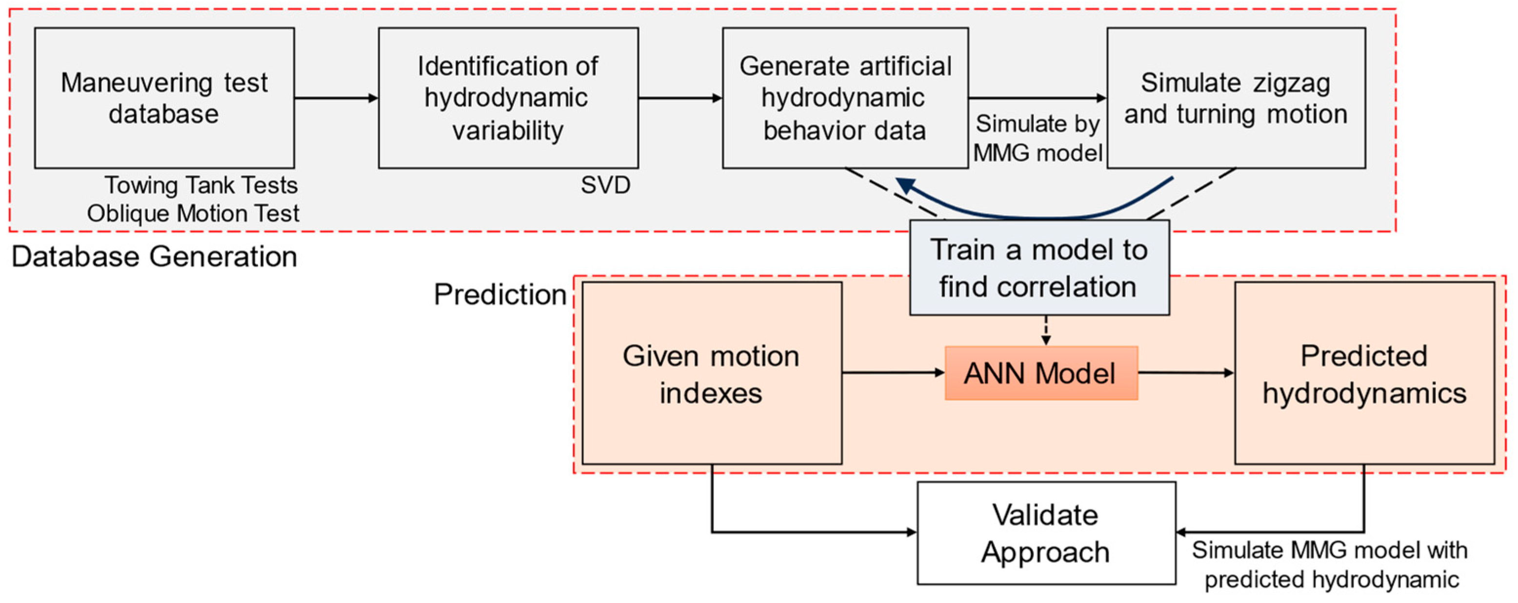
In the present study, a ship hydrodynamic behavior prediction method is proposed to build a ship maneuvering model. The proposed methodology can be considered in three stages. In the first stage, an existing hydrodynamics database was used to extract the hydrodynamic variability of vessels, and artificial hydrodynamic behaviors were generated using hydrodynamic variation vectors. Using the MMG model, the turning and zigzag characteristics of the target ship with artificial hydrodynamic behaviors were obtained. In the second stage, an artificial neural network model was built to predict the weight of each hydrodynamic variation. In the third stage, the performance of the proposed methodology was evaluated by comparing the given turning/zigzag indexes and simulated motion of the target ship, whose hydrodynamic behavior was obtained by using an artificial neural network model. The overview of the presented methodology is given in Figure 1.
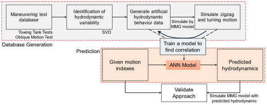
Figure 1.
The workflow of the proposed approach.
2.1. Ship Dynamics Model
First, a ship dynamic model, namely the MMG model, was created to investigate the maneuvering behavior of a ship. The equation of motion is given in Equation (1), where m, mx, and my are the mass and added mass components in the x- and y-directions, Izz and Jzz are the inertia and added inertia term in the yaw direction with respect to the center of gravity, uG, vG, and rG are ship speeds in the surge, sway, and yaw directions, and X, Y, and N are acting forces and moments in relation to a ship.
The resultant forces and moments, X, Y, and N, consist of hull, propeller, and rudder components. Forces regarding hull, propeller, and rudder are denoted by H, P, and R, respectively, as given in Equation (2).
Hull forces, which are the focus of the study, are defined as a summation of straight moving resistance, R0, and maneuvering resistance. Straight moving resistance, R0, can be predicted using empirical formulas with high accuracy. In the present study, straight moving resistance is predicted by using the Holtrop–Mennen model [9] and Schoenherr’s method [22]. On the other hand, maneuvering forces are usually determined by towing tank experiments. The magnitude of forces exerted on a ship is determined via polynomial functions of drift, β = sin−1(vG/U), and nondimensional yaw rate r′ = r(L/U), as given in Equation (3), where ρ is the density of water, L is the length of ship, d is the draft of a ship, U is the resultant speed, m′x and m′y are normalized added mass by (1/2)ρL2d, x′G is the normalized location of the center of gravity by L, and X′ββ, X′βr, X′rr, X′ββββ, Y′β, Y′r, Y′βββ, Y′ββr, Y′βrr, Y′rrr, N′β, N′r, N′βββ, N′ββr, N′βrr, and N′rrr are hydrodynamic derivatives.
The propeller force was calculated as shown in Equation (4) by assuming that the propeller only generates thrust, where t is the thrust reduction factor, nP is the propeller revolution, DP is the propeller diameter, and KT is the thrust coefficient which is determined via the advanced ratio JP.
The rudder force was evaluated by using Equation (5) where xR is the rudder position, tR, aH, and xH are the interaction parameters between the hull and rudder, FN is the normal force of the rudder, and δ is the rudder angle.
Further details of the MMG model can be found in [6].
2.2. Determination of Orthonormal Base Vectors and Generating Artificial Hydrodynamic Characteristics
The present study focuses on the hull hydrodynamic forces and corresponding hydrodynamic derivatives. Hydrodynamic force, as given in Equation (3), is defined in terms of polynomial functions, whose coefficients are determined through experiments. Different hull forms and dimensions lead to various hydrodynamic variations. When hydrodynamic coefficients were defined as independent variables in each direction, the relation between the hull form and hydrodynamic forces was lost. In other words, when the hull form or size of the ship slightly changed, the hydrodynamic forces in each direction varied. Thus, it is essential to evaluate all hydrodynamic coefficients as a whole in system identification problems. Another important point is that hydrodynamic forces are defined as polynomial functions, whose bases are not orthogonal. Thus, the inverse problem of finding hydrodynamic behavior using motion data may fail. The present study proposes new orthogonal base vectors which were obtained using the SVD of an experimental maneuvering database.
In order to understand the hydrodynamic variations, a hydrodynamic parameters database for the MMG model [23] was used. The database contains 32 different hydrodynamic behaviors of the 30 different ships including tankers, bulk carriers, containerships, PCCs, and fishery vessels. The database is a collection of captive model tests conducted by various researchers, and the hydrodynamic parameters were calculated as explained in a previous study [6]. In the present study, 20 hydrodynamic characteristics were used excluding the fishery vessels and ferries, ships with trim, and ships having twin propellers. The main particulars, experimentally obtained hydrodynamic derivatives, and interaction coefficients of the ships in the database are given in Table 1.

Table 1.
Main particulars, hydrodynamic derivatives, and interaction coefficients of the ships. Adapted from [23].
In order to obtain the orthogonal base vectors, the presented data in Table 1 have undergone some mathematical operations. First, X′H, Y′H, and N′H of each ship were calculated without considering R0, which can be calculated using empirical formulas, between ranges of ±20 degrees for β and ±0.8 for r′, as given in Equation (6).
Then, the matrices which describe the hydrodynamic behavior of the ith ship, X′H,i, Y′H,i, and N′H,i, were combined into one vector, hi, by including the interaction coefficients as given in Equation (7). Since the number of interaction coefficients is considerably lower than the number of entries in the matrices given in Equation (6), the interaction coefficients of each ship were repeated 10 times to balance the effects of interaction coefficients and maneuvering behavior.
After defining the hydrodynamics of each ship, the average hydrodynamics of all ships, have, in the database was found. Then, the hydrodynamic variation matrix, , whose columns were obtained as the difference between the hydrodynamic behavior of the ith ship, hi, and the average hydrodynamic behavior, have, was built as given in Equation (8).
The matrix, , explains how each ship varies from the mean hydrodynamic behavior. The SVD of the hydrodynamic variation matrix, , yields three different matrices: U, which shows column wise orthonormal characteristics; Σ, which shows how dominant each vector is; and V which shows the row wise orthonormal characteristics, using Equation (9). Each column of matrix U, ui, is ordered according to dominance. The contribution of each variation, λi, can be found as the ratio of the square of the ith diagonal entry of matrix, Σ, to the summation of the square of each diagonal entry of the matrix, Σ, using Equation (10).
Considering the cumulative contribution of the first nmode modes, which expresses more than 95% of all variations, an artificial hydrodynamic behavior generator was created. For this purpose, a coefficient matrix C was defined as the multiplication of Σ and VT. The average value of each row vector was almost zero, since the mean behavior was subtracted from the hydrodynamic variation matrix, Hvar. Then, standard deviation in each row vector entries, σi, was found, and an artificial hydrodynamic characteristic generator was created as given in Equation (11), where hgen is the generated hydrodynamic behavior, and xi is the weight of the ith mode, ui, which is the ith column of matrix U.
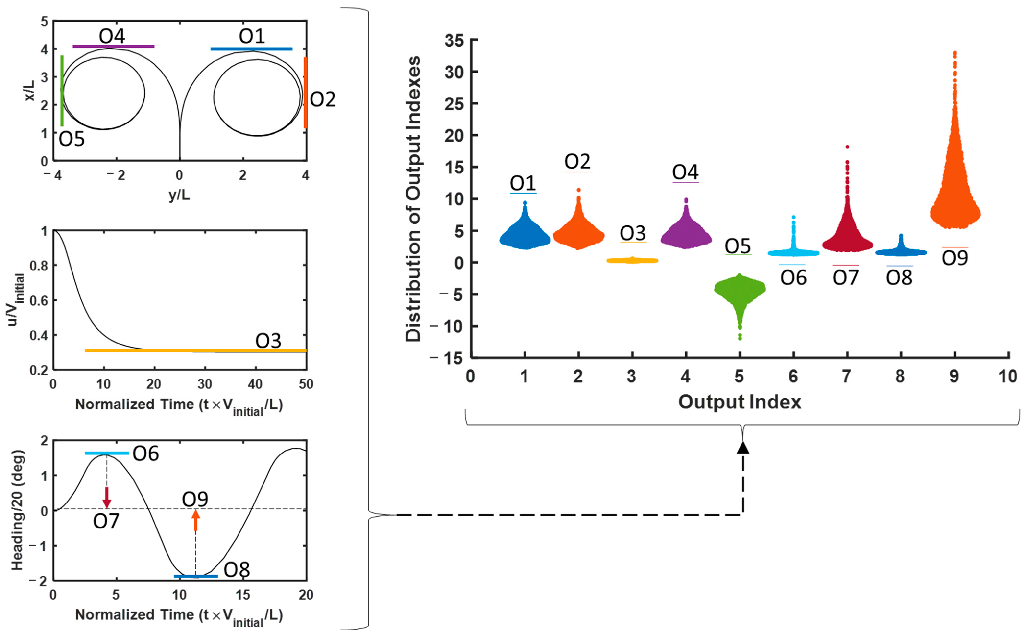
Then, many artificial hydrodynamic behaviors were generated for the target ships by using randomized weights xi within the range of ±3 standard deviations. Using the generated hydrodynamic behaviors and main particulars of the ship, turning tests (±35 degrees) and zigzag tests (+20/−20 degrees) were simulated via the MMG model, and the motion variations were obtained. In order to describe the motion, the motion index, qi, was defined in a normalized manner, as given in Equation (12), where AD is the advance, DT is the tactical diameter, Uinitial and Ufinal are the initial and final steady ship speeds during turning, OS1 and OS2 are the first and second overshoot angles during zigzag maneuvers, and t1 and t2 are the corresponding time of the first and second overshoots.
2.3. Artificial Neural Network Model to Predict Hydrodynamic Characteristics Based on the Motion Index
The next step in the algorithm is to model the relationship between the motion and corresponding coefficients which yields what kind of hydrodynamics can provide such maneuverability. Since the relation between hydrodynamic characteristics and turning/zigzag maneuvering behavior is quite complex and nonlinear, artificial neural network models were used.
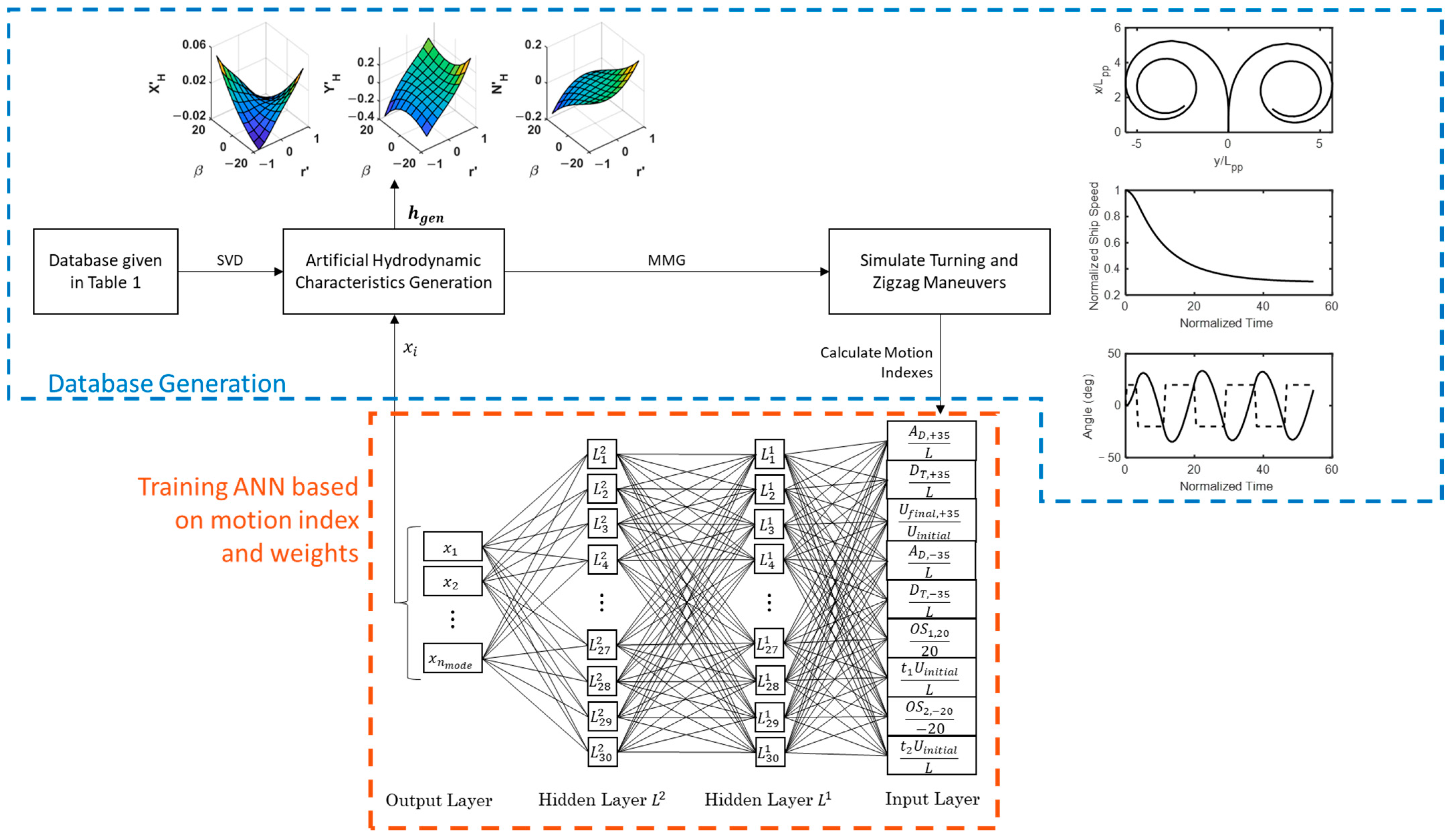
Hydrodynamic characteristics were generated via randomized weights for each mode, xi, forming the output layer of the artificial neural network model. Then, artificial hydrodynamic behavior vector, hgen, was calculated based on Equation (11). Through randomly generating numerous hydrodynamic behaviors, a database of hydrodynamic behavior was formed. Using the hydrodynamic behavior database and target ship specifications, turning and zigzag maneuvering simulations were conducted using the MMG model. Finally, motion indexes, q, were obtained for each simulation, and an artificial neural network model was trained to predict which weight vector, x, corresponds to a given motion index, q. The workflow is given in Figure 2.
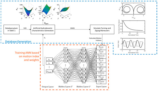
Figure 2.
Database generation and training the artificial neural network model to predict weights for given motion index.
It should be noted that all the indexes except Ufinal,+35/Uinitial were updated using the natural logarithm of their absolute values, since all the motion indexes except Ufinal,+35/Uinitial showed a skewed distribution. An artificial neural network model was trained with inputs of motion index, qi, and outputs of weight vector, x.
3. Results
First of all, the data given in Table 1 were transformed into data points of the maneuvering resistance specified in Equation (3), whose inputs are drift angle, β, and non-dimensional yaw rate, r′ and outputs are non-dimensional force and moment components, (XH + myvGrG − R0)/((ρ/2)LdU2), (YH − mxuGrG)/((ρ/2)LdU2), and NH/((ρ/2)L2dU2). In the generation of datapoints, the sampling points of the drift angle, β, and non-dimensional yaw rate were determined as –20, –15, –10, …, 10, 15, 20 degrees, and –0.8, –0.6, …, 0.6, 0.8, respectively. Then, the hydrodynamic variability matrix, Hvar, was obtained by following the prescribed steps through Equation (3) to Equation (8).
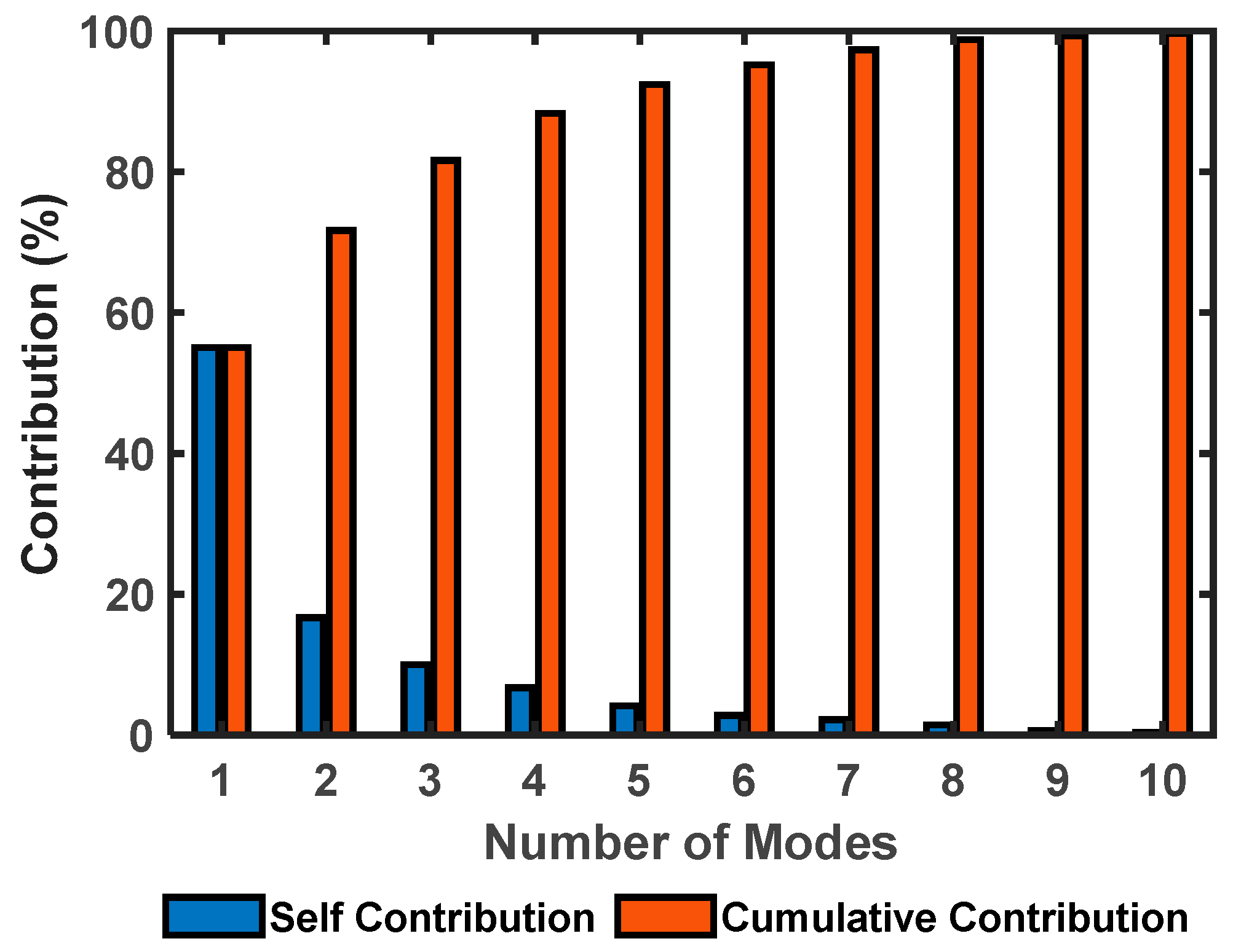
The singular value decomposition of the matrix Hvar led to several orthonormal modes of hydrodynamic variations in a descending order of self-contribution. Figure 3 shows the self and cumulative contributions of each mode. According to Figure 3, only the first mode expresses more than 50% of the hydrodynamic variations, and the cumulative contribution of the first six modes reaches 95%.

Figure 3.
The self and cumulative contribution of each hydrodynamic variation mode.
Then, the mean value and ranges of the minimum and maximum coefficients of each corresponding mode were calculated for the first six modes, as given in Figure 4. Since the mean hydrodynamic behavior was subtracted in the matrix Hvar, the mean values of the coefficients were zero. To determine the upper and lower bounds of the coefficients used in the artificial hydrodynamic behavior generator, the standard deviation of each coefficient was calculated.
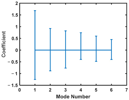
Figure 4.
The mean value and standard deviation of coefficients of each mode.
In order to predict the hydrodynamic behavior of a ship, numerous artificial hydrodynamic behaviors were generated for randomly varying xi values in Equation (11). Since straight moving resistance was not included in the artificial hydrodynamic behavior generator, empirical formulas were used for the straight moving resistance.
3.1. The Prediction of the Hydrodynamic Behavior of KVLCC2
In the first example, the target ship was selected as KVLCC2, whose main particulars are given in Table 2. A total of 2603 artificial hydrodynamic behaviors were generated and straight moving resistance, R0, was added to the X force component. Then, the MMG model was used to simulate how different artificial hydrodynamic behaviors would change the turning and zigzag maneuvering parameters, as given in Figure 5. It was found that the generated hydrodynamic behaviors resulted in a wide range of turning and zigzag motion patterns. As shown in the distribution of the output indexes in Figure 5, all the output indexes (O1–O9) but the third index (O3—yellow) showed a skewed distribution, which may reduce the performance of the generalization capabilities of artificial neural networks. Therefore, all the output indexes except the third index (O3—yellow) were updated using the logarithm of their absolute values, and the skewness of the distribution of output indexes was reduced.
Table 2.
Main particulars and other parameters of KVLCC2.

Figure 5.
Motion indexes of a simulated motion and the distribution of each output index.
After obtaining the updated output indexes, the mean output indexes were stored and subtracted from the output indexes and normalized via standard deviations. Since the purpose of the study was to predict what kind of hydrodynamics the target ship has based on the turning and zigzag maneuvering characteristics, an artificial neural network model was trained to express the behavior between the motion indexes and input coefficients, xi.
First, the dataset was split into training, test, and validation sets with a percentage of 70, 15, and 15, respectively. The input layer and output layer were connected to each other using two hidden layers with 30 neurons for each. The performance of the neural network model was calculated using the metric of mean squared error, and an early stopping technique was adopted to eliminate the overfitting.
The full-scale simulation results conducted by Yasukawa and Yoshimura [6], given in Table 3, were used to predict what kind of hydrodynamic behavior leads to such motion. Since the speed reduction was not given explicitly, it was assumed that Ufinal/Uinitial was 0.3. Then, the given motion indexes were updated for normalization, and the coefficients of hydrodynamic variations were found. Then, the turning and zigzag tests were repeated using the predicted hydrodynamic behavior data.
Table 3.
Motion indexes of the target ship, KVLCC2.
The comparison between the simulated motion by using the predicted hydrodynamic behavior, shown in red solid lines, and the given motion indexes in Table 3, shown in black dashed lines, is given in Figure 6. According to Figure 6, the artificial neural network model provided reasonable hydrodynamic behavior data which resulted in a significantly similar motion with the given motion indexes. Especially, the tactical diameters and speed reduction during turning, and overshoot angles and timing during zigzag maneuvering showed significant similarity. On the other hand, the advances during the turning test exhibited larger values than the given motion index.
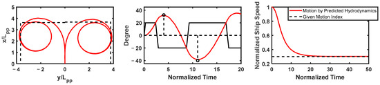
Figure 6.
Comparison of the motion obtained via the predicted hydrodynamics, shown in red solid line, and given motion index parameters, shown by black dashed line.
3.2. The Prediction of the Hydrodynamic Behavior of a Virtual Ship
Since KVLCC2 was in both the training dataset and used for exemplification of the proposed methodology, the performance of the proposed methodology might not be evaluated accurately. Therefore, a virtual ship was considered by assuming the following main particulars given in Table 4, where L, B, and T are the length, breadth, and draft of the virtual ship, D is the diameter of the propeller, H and AR are the rudder height and area, xG is the position of the center of mass according to the mid-ship coordinates, k0, k1, and k2 are the polynomial coefficients of the J (advance ratio)-KT (thrust coefficient), t is the thrust deduction factor, and Vinitial is the initial ship speed.
Table 4.
Main particulars and other parameters of the virtual ship.
The added mass and inertia of the virtual ship were predicted based on the previous study [24,25]. The inertia of the ship was predicted so that the radius of yaw gyration is 0.25 × L. Since it is a virtual ship, its different given motion indexes were assumed, as given in Table 5.
Table 5.
Three examples of the different motion patterns of a virtual ship.
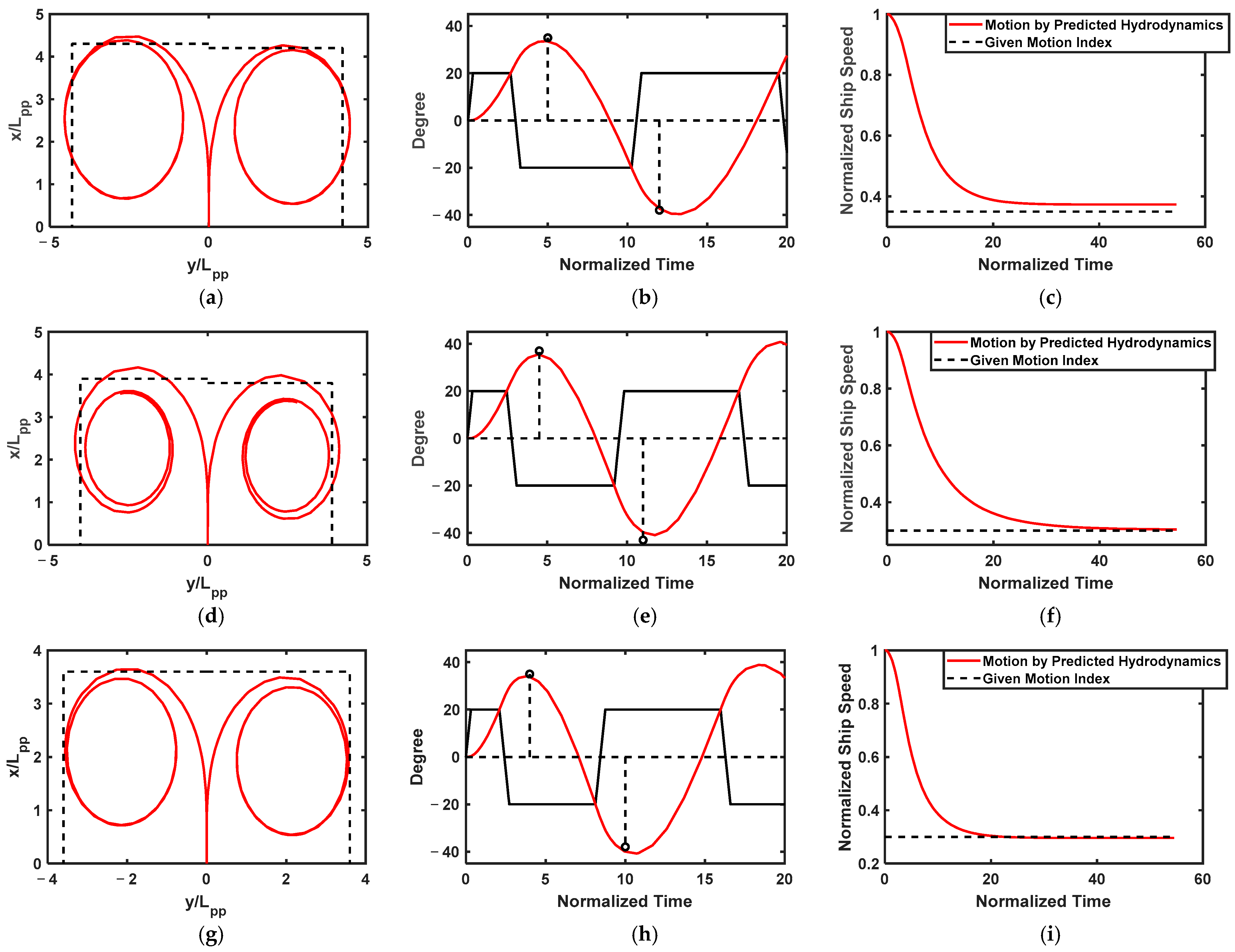
Regarding the virtual ship, a total of 1405 turning and zigzag simulations were conducted, and motion indexes, qi, and input indexes, xi, were obtained. The relation between the input and output layers was modeled by using artificial neural networks with two hidden layers with 30 neurons in each. After training the artificial neural network model, the hydrodynamic behavior of three example turning and zigzag characteristics, given in Table 5, were predicted. Based on the predicted hydrodynamic behavior, the turning and zigzag characteristics were obtained and compared with the given motion indexes, as shown in Figure 7.
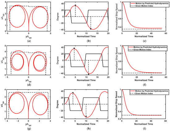
Figure 7.
The performance of the proposed methodology tested by using a virtual ship and given motion indexes (a–c) M01, (d–f) M02, and (g–i) M03.
As shown in Figure 7, the predicted hydrodynamics resulted in a motion which exhibited strong agreement with the given motion indexes. Especially the speed reduction during the turning test and first overshoot angle and timing highly correlated with the given motion indexes. On the other hand, the predicted hydrodynamics in some cases produced a slightly larger advance and tactical diameter compared to the given motion indexes.
4. Discussion
The recent efforts on decarbonization and autonomous shipping in the maritime industry require the digitalization of the industry and simulation-based techniques. To investigate how a ship responds to different kinds of modifications such as wind sails, air lubrication systems, controllable pitch propellers, etc., it is essential to model the ship dynamics. One of the core elements in ship dynamics is the hydrodynamic behavior of the ship. While there are many reliable resistance prediction methods for commercial vessels, the studies on the prediction of maneuvering behavior are limited. The present study proposes a system identification methodology to understand how maneuvering resistance varies depending on the given performance of turning and zigzag tests.
The conventional way of acquiring hydrodynamic behavior is the towing tank experiments, which require a significant amount of time and money. Another methodology used in previous studies relies on the time series data of operating ships. However, the hydrodynamic behaviors and operational data of commercial vessels are usually kept confidential, and this puts a burden on technological development. The present study, for this reason, focuses on the prediction of hydrodynamic behavior using general motion indexes that are investigated by classification societies.
In the proposed methodology, an SVD-based characterization of ship hydrodynamics was utilized instead of the polynomial description used in the existing studies. One of the main reasons for this is to hold the behavioral integrity among the directions in surge, sway, and yaw; in other words, each input coefficient, xi, affects all hydrodynamics unlike the hydrodynamic derivatives, X′ββ, X′βr, X′rr, X′ββββ, Y′β, Y′r, Y′βββ, Y′ββr, Y′βrr, Y′rrr, N′β, N′r, N′βββ, N′ββr, N′βrr, and N′rrr, used in Equation (3). Furthermore, the hydrodynamic derivatives were defined based on the polynomial basis functions, which are not orthogonal. In the SVD-based characterization, all the hydrodynamic variations are expressed in a way that is orthogonal. Therefore, an SVD-based characterization requires less variables to express the hydrodynamics of ships and forms a suitable system to generate artificial yet realistic hydrodynamic behavior. Due to the given reasons, SVD-based hydrodynamic behavior generation provides realistic hydrodynamic behaviors with a unique expression by orthonormal variation modes using less variables over the generation of hydrodynamic characteristics using polynomial-based methods.
Through generating a large number of artificial hydrodynamics data, the connection between motion and the corresponding hydrodynamic behavior can be built using artificial neural networks. In the present study, two examples of the prediction of hydrodynamic behavior were shown based on the given motion indexes. In both examples, the motion obtained by the predicted hydrodynamics data demonstrated a high correlation with the given motion indexes. Although the proposed methodology showed a good performance in general, the prediction accuracy of the advance during turning was relatively lower than the prediction accuracy of the other indexes. The main reason could be the resistance model which was predicted by commonly used empirical methods. Since ship speed is the maximum initially and reduces gradually, the advance is significantly affected by the resistance model. Through improving the resistance model, the prediction accuracy of the proposed model would expect to be increased.
Although many advantages of the proposed methodology were shown, there are some drawbacks as well. The proposed methodology highly depends on the data used in the extraction of orthogonal hydrodynamic variation vectors. As explained in the Methods section, only certain types of ships were selected to extract the features regarding hydrodynamic variability. If all ships were included in the feature extraction, it would be expected that ship type-specific variations would dominate the hydrodynamic variability. In order to capture the hydrodynamic variability within similar ship types, the present study considers certain ships to express ship-specific hydrodynamic variability. Thus, it is essential to use as much hydrodynamic data as possible and to limit the type of ships.
In future studies, the proposed methodology will be expanded to generalize ship hydrodynamics to be used in the decision-making process and design exploration studies. Also, the application of the proposed methodology on the adoption of different systems on existing vessels to determine decarbonization pathway will be demonstrated for different ship designs. Another research direction will be the elimination of the environmental effects on maneuvering performance of full-scale ships to find out the real performance in calm water.
5. Conclusions
Recent regulations in the maritime industry have made digitalization more and more necessary. The performance evaluation of the different vessels is one of the topics regarding digitalization. Up to date, the hydrodynamic behavior of ships was usually predicted based on empirical models, extensive experiments, and computational fluid dynamics simulations. Unlike the existing methodologies, the present study proposes a hybrid approach which combines the existing experimental datasets to understand the hydrodynamic variability, and a prediction methodology of hydrodynamic behavior based on the given motion indexes by generating artificial hydrodynamic characteristics. The proposed methodology can be summarized as follows:
- Create/Use an experimental or computational database for hydrodynamic characteristics of many ships;
- Form the hydrodynamic behavior vectors, hi, for each ship;
- Calculate the mean hydrodynamic behavior vector of all ships, have;
- Create the hydrodynamic variation matrix, Hvar;
- Apply singular value decomposition to the hydrodynamic variation matrix, Hvar;
- Generate artificial hydrodynamic characteristics using the random weight vector, x, standard deviations of each coefficient, σ, mean hydrodynamic behavior vector, have, and orthonormal hydrodynamic variation vector, u;
- Create a simulation-based turning and zigzag maneuvering database which contains random weight vectors, xi, and motion index, qi, using the MMG model;
- Train an artificial neural network for the target ship to predict which weight vector, x, corresponds to the given motion index, q.
The proposed methodology has several advantages and limitations in examining the hydrodynamic behavior of target ships. Since the proposed methodology uses singular value decomposition-based variation modes, it requires fewer parameters than conventional approaches to describe ship hydrodynamics which reduces both the cost and time required compared to experimental investigations and computational fluid dynamics simulations. Also, variation vectors obtained by using SVD are orthonormal and derived from experimental databases; therefore, SVD-based hydrodynamic behavior generation forms uniquely represented artificial and realistic hydrodynamic behaviors. This property allows artificial neural network models to perform better in correlating the motion and hydrodynamic variability. On the other hand, experimental or computational database used in SVD introduces the issue of data dependency. Future studies will be conducted to eliminate the issue of data dependency and expand the idea to find out the relation among hull shape, hydrodynamic behavior, and motion.
Finally, the performance of the proposed method was tested considering two target ships, and the motion using predicted hydrodynamics showed a strong agreement with the given motion indexes. It shows that the proposed methodology allows researchers and engineers in the field to establish digital models of the target ships rapidly.
Funding
This research received no external funding.
Institutional Review Board Statement
Not applicable.
Informed Consent Statement
Not applicable.
Data Availability Statement
Data are contained within the article.
Acknowledgments
I would like to thank Hironori Yasukawa for the support and advice. Also, I would like to thank the Maritime and Ocean Digital Engineering (MODE) Laboratory members at the University of Tokyo for their research advice.
Conflicts of Interest
The author declares no conflicts of interest.
Abbreviations
The following abbreviations are used in this manuscript:
| CFD | Computational fluid dynamics |
| GHG | Greenhouse gases |
| MMG | Maneuvering modeling group |
| SVD | Singular value decomposition |
Symbols
The following abbreviations are used in this manuscript:
| AD | Advance during turning |
| AR | Rudder area |
| B | Breadth of the ship |
| CB | Block coefficient |
| d | Draft of the ship |
| DP | Diameter of the propeller |
| DT | Tactical diameter during turning |
| FN | Rudder normal force |
| H | Height of the rudder |
| have | Average hydrodynamic behavior vector |
| hgen | Generated hydrodynamic behavior vector |
| hi | Hydrodynamic behavior vector of the ith ship |
| Hvar | Hydrodynamic variation matrix |
| Izz | Moment of inertia of the ship around the z-axis |
| Jzz | Added moment of inertia of the ship around the z-axis |
| L | Length of the ship |
| m | Mass of the ship |
| mx, my | Added masses of the ship in the x- and y-directions |
| N | Total acting moment in the z-direction |
| N′βββ, N′ββr, etc. | Nondimensional hydrodynamic derivatives in the z-direction |
| nP | Propeller revolution |
| OS1 | First overshoot angle of the ship during a zigzag maneuver |
| OS2 | Second overshoot angle of the ship during a zigzag maneuver |
| q | Motion index vector |
| r | Yaw rate with respect to the mid-ship reference frame |
| R0 | Straight moving resistance |
| rG | Yaw rate with respect to the center of gravity |
| t | Thrust reduction factor |
| t1 | Corresponding time of the first overshoot during a zigzag maneuver |
| t2 | Corresponding time of the second overshoot during a zigzag maneuver |
| tR, aH, xH | Rudder–hull interaction parameters |
| u | Surge speed with respect to the mid-ship reference frame |
| U | Resultant ship speed |
| Ufinal | Final steady speed of the ship during turning |
| uG | Surge speed with respect to the center of gravity |
| ui | The ith orthonormal hydrodynamic variation vector |
| Uinitial | Initial speed of the ship during turning |
| v | Sway speed with respect to the mid-ship reference frame |
| vG | Sway speed with respect to the center of gravity |
| X | Total acting force in the x-direction |
| x | Weight vector |
| X′H, Y′H, N′H | Hydrodynamic behavior matrices |
| X′ββ, X′βr, etc. | Nondimensional hydrodynamic derivatives in the x-direction |
| xG | The position of the center of gravity with respect to the mid-ship reference frame |
| XH, YH, NH | Hull forces and moments |
| xi | Weight of the ith mode |
| XP, YP, NP | Propeller forces and moments |
| xR | Rudder position |
| XR, YR, NR | Rudder forces and moments |
| Y | Total acting force in the y-direction |
| Y′βββ, Y′ββr, etc. | Nondimensional hydrodynamic derivatives in the y-direction |
| β | Drift |
| γR+, γR− | Flow straightening coefficient |
| δ | Rudder angle |
| ε | The ratio of wake fraction for the propeller and rudder positions |
| ρ | Density of water |
| σi | Standard deviation of the coefficient of the ith mode |
References
- IMO. 2023 IMO Strategy on Reduction of GHG Emissions from Ships. Available online: https://www.imo.org/en/OurWork/Environment/Pages/2023-IMO-Strategy-on-Reduction-of-GHG-Emissions-from-Ships.aspx?refresh=1 (accessed on 5 February 2025).
- Tillig, F.; Ringsberg, J.W.; Mao, W.; Ramne, B. Analysis of Uncertainties in the Prediction of Ships’ Fuel Consumption—From Early Design to Operation Conditions. Ships Offshore Struct. 2018, 13, 13–24. [Google Scholar] [CrossRef]
- Ogawa, A.; Koyama, T.; Kijima, K. MMG report-I, on the mathematical model of ship manoeuvring. Bull. Soc. Nav. Archit. Jpn. 1977, 575, 22–28. [Google Scholar]
- Ogawa, A.; Kasai, H. On the Mathematical Model of Manoeuvring Motion of Ships. Int. Shipbuild. Prog. 1978, 25, 306–319. [Google Scholar] [CrossRef]
- Inoue, S.; Hirano, M.; Kijima, K.; Takashina, J. A practical calculation method of ship maneuvering motion. Int. Shipbuild. Prog. 1981, 28, 207–222. [Google Scholar] [CrossRef]
- Yasukawa, H.; Yoshimura, Y. Introduction of MMG Standard Method for Ship Maneuvering Predictions. J. Mar. Sci. Technol. 2015, 20, 37–52. [Google Scholar] [CrossRef]
- Taimuri, G.; Matusiak, J.; Mikkola, T.; Kujala, P.; Hirdaris, S. A 6-DoF Maneuvering Model for the Rapid Estimation of Hydrodynamic Actions in Deep and Shallow Waters. Ocean Eng. 2020, 218, 108103. [Google Scholar] [CrossRef]
- Ren, Z.; Han, X.; Yu, X.; Skjetne, R.; Leira, B.J.; Sævik, S.; Zhu, M. Data-Driven Simultaneous Identification of the 6DOF Dynamic Model and Wave Load for a Ship in Waves. Mech. Syst. Signal Process. 2023, 184, 109422. [Google Scholar] [CrossRef]
- Holtrop, J.; Mennen, G.G.J. An Approximate Power Prediction Method. Int. Shipbuild. Prog. 1982, 29, 166–170. [Google Scholar] [CrossRef]
- Zhang, C.; Liu, X.; Wan, D.; Wang, J. Experimental and Numerical Investigations of Advancing Speed Effects on Hydrodynamic Derivatives in MMG Model, Part I: Xvv,Yv,Nv. Ocean Eng. 2019, 179, 67–75. [Google Scholar] [CrossRef]
- Yao, J.; Cheng, X.; Liu, Z. Ship manoeuvring prediction based on numerical towing tank technique. Int. J. Marit. Eng. 2018, 160. [Google Scholar] [CrossRef]
- Yao, J.; Liu, Z.; Song, X.; Su, Y. Ship Manoeuvring Prediction with Hydrodynamic Derivatives from RANS: Development and Application. Ocean Eng. 2021, 231, 109036. [Google Scholar] [CrossRef]
- Xu, H.; Soares, C.G. Hydrodynamic Coefficient Estimation for Ship Manoeuvring in Shallow Water Using an Optimal Truncated LS-SVM. Ocean Eng. 2019, 191, 106488. [Google Scholar] [CrossRef]
- Costa, A.C.; Xu, H.; Guedes Soares, C. Robust Parameter Estimation of an Empirical Manoeuvring Model Using Free-Running Model Tests. J. Mar. Sci. Eng. 2021, 9, 1302. [Google Scholar] [CrossRef]
- Yoshimura, Y.; Masumoto, Y. Hydrodynamic Database and Manoeuvring Prediction Method with Medium High-Speed Merchant Ships and Fishing Vessels. In Proceedings of the International MARSIM Conference, Singapore, 23–27 April 2012; pp. 1–9. [Google Scholar]
- Kijima, K.; Katsuno, T.; Nakiri, Y.; Furukawa, Y. On the Manoeuvring Performance of a Ship with Theparameter of Loading Condition. J. Soc. Nav. Archit. Jpn. 1990, 1990, 141–148. [Google Scholar] [CrossRef] [PubMed]
- Alexandersson, M.; Mao, W.; Ringsberg, J.W. System Identification of Vessel Manoeuvring Models. Ocean Eng. 2022, 266, 112940. [Google Scholar] [CrossRef]
- Luo, W.; Guedes Soares, C.; Zou, Z. Parameter Identification of Ship Maneuvering Model Based on Support Vector Machines and Particle Swarm Optimization. J. Offshore Mech. Arct. Eng. 2016, 138, 031101. [Google Scholar] [CrossRef]
- Wang, T.; Li, G.; Wu, B.; Æsøy, V.; Zhang, H. Parameter Identification of Ship Manoeuvring Model under Disturbance Using Support Vector Machine Method. Ships Offshore Struct. 2021, 16, 13–21. [Google Scholar] [CrossRef]
- Xue, Y.; Liu, Y.; Xue, G.; Chen, G. Identification and Prediction of Ship Maneuvering Motion Based on a Gaussian Process with Uncertainty Propagation. J. Mar. Sci. Eng. 2021, 9, 804. [Google Scholar] [CrossRef]
- Kanazawa, M.; Wang, T.; Ichinose, Y.; Skulstad, R.; Li, G.; Zhang, H. Bridging Similar Ships’ Dynamics for Safeguarding the System Identification of Maneuvering Models. Ocean Eng. 2023, 280, 114874. [Google Scholar] [CrossRef]
- Schoenherr, K.E. Resistance of Flat Surfaces Moving Through a Fluid; Johns Hopkins University: Baltimore, MD, USA, 1932. [Google Scholar]
- Yoshimura, Y.; Nakamura, M.; Taniguchi, T.; Yasukawa, H. Empirical Formulas of Hydrodynamic Parameters for Predicting Ship Maneuvering Based in MMG-Model. Ocean Eng. 2025. under review. [Google Scholar]
- Zhou, Z.; Yan, S.; Feng, W. Manoeuvring prediction of multiple-purpose cargo ships. Ship Eng. 1983, 6, 21–36. [Google Scholar]
- Liu, J.; Hekkenberg, R.; Quadvlieg, F.; Hopman, H.; Zhao, B. An Integrated Empirical Manoeuvring Model for Inland Vessels. Ocean Eng. 2017, 137, 287–308. [Google Scholar] [CrossRef]


Disclaimer/Publisher’s Note: The statements, opinions and data contained in all publications are solely those of the individual author(s) and contributor(s) and not of MDPI and/or the editor(s). MDPI and/or the editor(s) disclaim responsibility for any injury to people or property resulting from any ideas, methods, instructions or products referred to in the content. |
© 2025 by the author. Licensee MDPI, Basel, Switzerland. This article is an open access article distributed under the terms and conditions of the Creative Commons Attribution (CC BY) license (https://creativecommons.org/licenses/by/4.0/).