LT-Sync: A Lightweight Time Synchronization Scheme for High-Speed Mobile Underwater Acoustic Sensor Networks

Abstract

Time synchronization is a crucial element of cooperativity among underwater acoustic sensor networks (UWASNs), and it plays an indispensable role in the application of and research into UWASNs. Although plenty of previous studies on time synchronization for UWASNs have been proposed and applied, most of them cannot perform well when the nodes have high mobility, and they are characterized by low energy efficiency. Tri-Message is a scheme proposed for networks in high-latency and resource-constrained environments, but it works unsatisfactorily when the nodes are movable. In that case, there is no such scheme for high-speed UWASNs with low energy consumption. Herein, we propose LT-Sync, a lightweight time synchronization scheme for high-speed mobile UWASNs. This adopts a Doppler-shift-estimating method to derive the propagation delay of high-speed UWASNs when the unsynchronized node moves uniformly in a single direction. In addition, an underwater spread-spectrum method is adopted for signal receiving to obtain the accurate Doppler shift. The simulation results show that LT-Sync is more feasible for high-speed UWASNs compared to existing methods and has high energy efficiency.

1. Introduction

In recent years, underwater acoustic sensor networks (UWASNs) have attracted a significant amount of research due to their great application potential; they are widely used in environmental monitoring, target tracking and disaster prevention [1,2]. Time synchronization plays an important role in UWASN applications [3]. However, the research into and application of time synchronization in UWASNs faces many challenges because of the defects of underwater acoustic (UWA) channels [4]. The greatest difference between the time synchronization of UWASNs and that of terrestrial wireless sensor networks is the huge propagation delay due to the different speeds of signal propagation. Furthermore, the nodes of UWASNs need to have a certain moving speed in some application scenarios [5], which leads to the possibility of the propagation delay changing in every communication process. More importantly, the sensor network energy efficiency directly affects the network performance. The computational capability of underwater node sensors is limited [6]; thus, it is inappropriate to design too-complex algorithms that have high computational demands.

The existing time synchronization algorithms for land-based sensors include fine-grained network time synchronization using reference broadcasts (RBS) [7], the timing-sync protocol for sensor networks (TPSN) [8], and the flooding time synchronization protocol (FTSP) [9]. However, none of them takes into account the special characteristics of the UWA environment, and they ignore the existence of propagation delays. Therefore, such protocols are not applicable to UWASNs.

Some research progress has been made in the time synchronization of UWASNs. TSHL [10] is a time synchronization protocol designed for UWA environments, which incorporates propagation delays into the algorithm design. This reduces the impact of clock drift rates on timing errors during high-latency timing; however, TSHL does not take into account the mutual movement between nodes. It is difficult for nodes of UWASNs to remain stationary, and the movement of nodes will also cause huge errors. MU-Sync [11] considers the relative movement of nodes based on TSHL and assumes the UWA channel as symmetric. However, the round-trip propagation delay in one of the synchronization processes is always different, and this assumption reduces the synchronization accuracy of the scheme.

D-Sync [12], DA-Sync [13], DE-Sync [14], and APE-Sync [15] all incorporate the Doppler shift caused by underwater mobile nodes into the synchronization process. They use it to calculate the propagation delay, thereby improving the accuracy of delay estimation in the case of nodes moving at low speeds. In these schemes, however, one synchronization process requires at least 25 exchanges of information, resulting in high energy consumption for the reference nodes that need to send a large number of synchronization signals. Tri-Message [16] is a lightweight time synchronization protocol, which applies only three messages in one synchronization process to estimate the clock skew and offset. However, it regards the propagation delays of three communication processes to be identical and ignores the existence of relativity between nodes.

Recently there have been some new time synchronization schemes for UWASNs. For example, an underwater network time synchronization method based on probabilistic graphical models [17] is suitable for large-scale networks. DC-Sync [18] is proposed for targeting complex moving underwater sensors, but the energy consumption is too high to be adopted in real-time UWASNs. SFDM [19] utilizes an unscented particle filter algorithm and an improved sound speed stratification effect compensation algorithm to improve the calibration accuracy of the array. All of them are able to improve the accuracy of time synchronization in UWASNs, but they are unable to be applied in UWASNs when sensor nodes are moving at high speeds.

Spread-spectrum communication is a widely adopted technique in underwater acoustic (UWA) channels [20,21,22], particularly through the use of a direct-sequence spread spectrum (DSSS). DSSS signals exhibit strong resilience in UWA communication, effectively mitigating noise and multipath interference [23]. Additionally, the dual differential spread-spectrum (DDSS) approach, implemented within the DSSS framework, enhances communication reliability even under mobile conditions [24]. Another advantage of DSSS is its ability to facilitate Doppler shift estimation during signal acquisition. In this method, a DSSS signal is generated by multiplying the data sequence with a spread-spectrum sequence before modulation onto a carrier wave. At the receiver, the original spread-spectrum sequence is required to successfully de-spread and recover the transmitted signal.

In this paper, based on the characteristics of the UWA channel, we propose LT-Sync, a lightweight time synchronization scheme for high-speed mobile UWASNs which uses the Doppler shift to estimate the node’s moving speed. In addition, it completes time synchronization with high accuracy, while its energy consumption is small. We use a parallel algorithm based on FFT for signal acquisition, and all the simulations are carried out based on BELLHOP.

The remainder of the paper is organized as follows. After introducing previous typical time synchronization schemes for underwater sensor networks, a description of the LT-Sync and system model is presented in Section 2. In Section 3, we introduce an acquisition method for receiving UWA spread-spectrum signals with a composite sequence. The simulation results and evaluation are included in Section 4. Finally, Section 5 concludes this paper.

2. Description of Time Synchronization Scheme

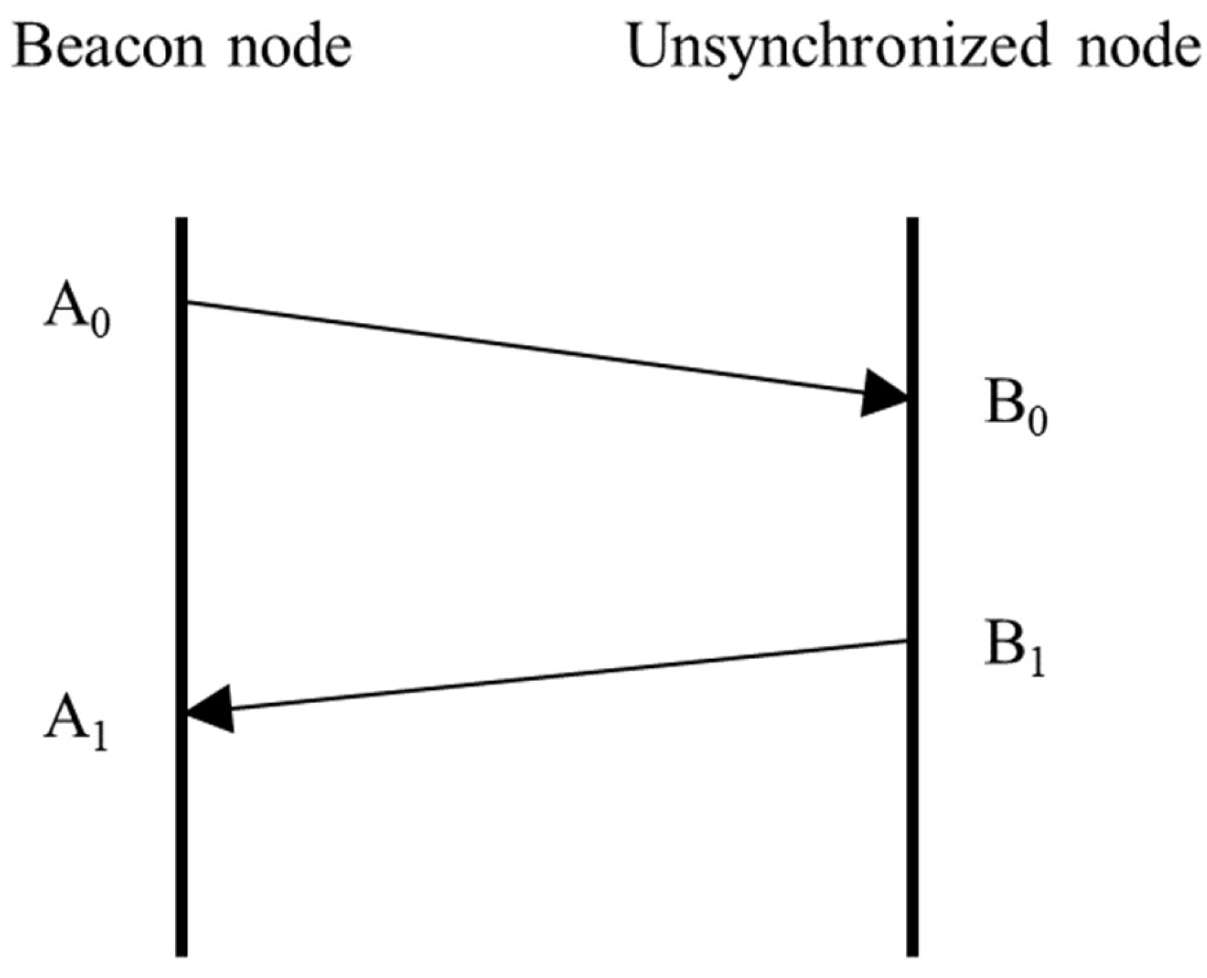
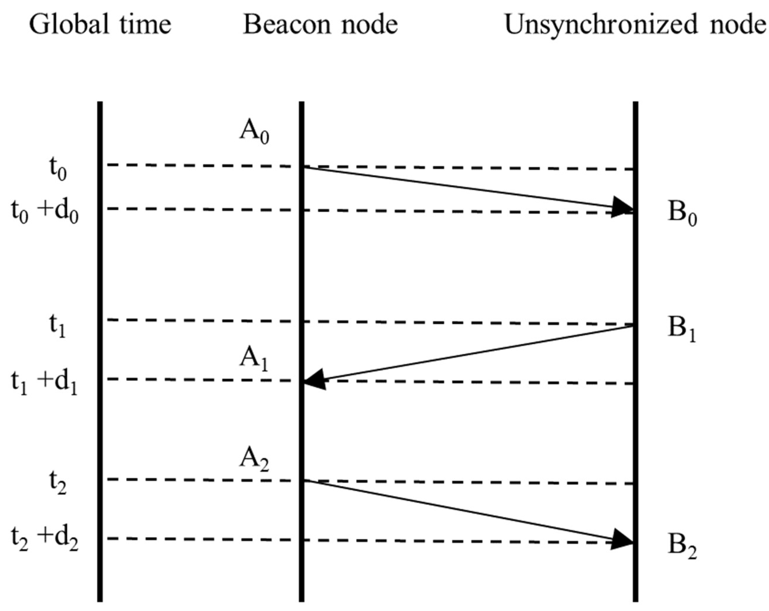
2.1. Synchronization Process

The basic principle of LT-Sync is the Sender–Receiver scheme, shown in Figure 1. A means beacon node and B means unsynchronized node.

We assume that A has no skew and offset error and B has unsynchronized clock skew α and offset β [25]. A first sends a synchronization message to B, and B sends its local time to A after obtaining the reference time. The time of any unsynchronized node is related to the reference time of the beacon node, as shown in (1):

$$B_i=\alpha A_i+\beta$$

(1)

where B_i denotes the local time of nodes at reference time A_i, and A_i represents the reference time of the beacon node. By denoting the delay at the first transmission as d₀ and the delay at the second transmission as d₁, the times of A and B during the two communications can be expressed as:

$$\left\{\begin{array}{c}{A}_0=t_0\\ B_0=\alpha (A_0+d_0)+\beta \\ B_1=\alpha t_1+\beta \\ A_1=t_1+d_1\end{array}\right.$$

(2)

where t₀ and t₁ denote the reference times of the first and second transmissions of the synchronization signal, respectively. The parameters α and β are needed for synchronization, but since four node times are known to calculate α and β, and only three node times are known to B after two communication processes, time synchronization cannot be completed. Therefore, we add another message exchange process and propose the LT-Sync message exchange scheme, shown in Figure 2.

Synchronization starts when the beacon node receives an external wake-up signal. Firstly, beacon node A sends a message to unsynchronized node B, including the captured timestamp A₀. When the synchronization message arrives at B, it captures its own receive timestamp B₀. Then, B saves the transmit timestamp B₁ and sends it to A after the waiting interval, and A records the receive timestamp A₁. Then, they swap their roles again. A sends the third message and puts the transmit timestamp A₂ together with A₁ in the message, and B receives the third message with the transmit timestamp B₂. Finally, all six timestamps are known to B: A₀, A₁, A₂, B₀, B₁, B₂. The relationship between them is given by the following equation:

$$\left\{\begin{array}{c}\begin{array}{c}{A}_0=t_0\\ B_0=\alpha (t_0+d_0)+\beta \\ B_1=\alpha t_1+\beta \end{array}\\ \begin{array}{c}{A}_1=t_1+d_1\\ A_2=t_2\\ B_2=\alpha (t_2+d_2)+\beta \end{array}\end{array}\right.$$

(3)

This yields the following expression for α and β:

$$\alpha ={\displaystyle \frac{B_2-B_0}{A_2-A_0+d_2-d_0}}$$

(4)

$$\beta ={\displaystyle \frac{(B_0+B_1)-\alpha \left(A_0+A_1+d_0-d_1\right)}{2}}$$

(5)

Tri-Message assumes that the three propagation delays are equal, so it is susceptible to obtaining α and β. However, in LT-Sync, the nodes move at high speed and there is a significant gap between three propagation delays, making the estimation of these delays a critical part of time synchronization.

2.2. Propagation Delay Estimation

LT-Sync utilizes the Doppler shift to estimate the movement speed of the unsynchronized node. According to the Doppler effect, when the wave source is stationary and the receiver is moving away from the source, the Doppler shift received at the receiver is related to the speed of the receiver [26], as follows:

$$v={\displaystyle \frac{\Delta f}{f}}c$$

(6)

In the formula, v denotes the speed of the unsynchronized node, c denotes the speed of sound in the UWA environment, f represents the initial frequency of the synchronization signal, and Δf is the Doppler shift obtained at the unsynchronized node.

To achieve accurate propagation delay estimation, we use the underwater node distribution scheme shown in Figure 3. Both of the nodes are distributed in an underwater environment with 10 m of depth, and the unsynchronized node moves in the direction away from the beacon node. When the synchronization process starts, the beacon node sends a synchronization message to the unsynchronized node, and the latter immediately makes a uniform linear motion at the current speed when it receives the synchronization message until the synchronization process is completed. Using this node-distribution scheme, we are able to obtain some significant parameters to calculate the clock skew and offset.

Here, l denotes the distance between two nodes when the beacon node sends the first message, and it can be obtained according to the time when the beacon node receives the first synchronization message echo. The three propagation delays are related to l according to (7):

$$\left\{\begin{array}{c}{d}_0={\displaystyle \frac{l}{c-v}}\\ d_1={\displaystyle \frac{l_1}{c}}\\ d_2={\displaystyle \frac{l+\left(A_2-A_0\right)v}{c-v}}\end{array}\right.$$

(7)

$$l_1=l+[B_1-(\alpha A_0+\beta )]v$$

(8)

In order to simplify the algorithm, we regard (αA₀ + β) as approximately equal to A₀. And from the results in Section 4, this does not significantly affect the accuracy of the algorithm. So, (7) can be simplified as (9):

$$\left\{\begin{array}{c}{d}_0={\displaystyle \frac{l}{c-v}}\\ d_1={\displaystyle \frac{l+(B_1-A_0)v}{c}}\\ d_2={\displaystyle \frac{l+\left(A_2-A_0\right)v}{c-v}}\end{array}\right.$$

(9)

Based on (6) and (9), the relationships between the propagation delays and the Doppler effect are expressed as:

$$\left\{\begin{array}{c}{d}_0={\displaystyle \frac{l}{c(1-\frac{\Delta f}{f})}}\\ d_1={\displaystyle \frac{l+(B_1-A_0)\frac{\Delta f}{f}c}{c}}\\ d_2={\displaystyle \frac{l+\left(A_2-A_0\right)\frac{\Delta f}{f}c}{c(1-\frac{\Delta f}{f})}}\end{array}\right.$$

(10)

The relationship between α, β and the Doppler shift can be obtained by (4) and (5):

$$\alpha ={\displaystyle \frac{\left(B_2-B_0\right)\left(1-\frac{\Delta f}{f}\right)}{\left(A_2-A_0\right)\left(1-\frac{\Delta f}{f}\right)+\left(A_2-A_0\right)\frac{\Delta f}{f}}}$$

(11)

$$\beta ={\displaystyle \frac{(B_0+B_1)-\alpha \left(\left(A_0+A_1\right)+\frac{\Delta f}{f}\left[\frac{l}{c(1-\frac{\Delta f}{f})}-\frac{\left(A_0-B_1\right)}{f}\right]\right)}{2}}$$

(12)

Thus, the process of propagation delay estimation has been completed, which used the Doppler shift to correct the clock skew and offset of the unsynchronized nodes that are moving at high speed. In that case, the whole process of LT-Sync can be summarized as follows:

(1)

To start with, the beacon node sends a wake-up signal, including the captured timestamp A₀, to the unsynchronized node. At the same time, the unsynchronized node immediately moves in a uniform straight line at its current speed and captures its own receive timestamp B₀.

(2)

Then, the unsynchronized node saves the transmit timestamp B₁ and sends it to the beacon node after a waiting interval, and the beacon node records the receive timestamp A₁. At the same time, the beacon node can obtain the Doppler shift by demodulating the signal from the unsynchronized node.

(3)

After that, the beacon node sends the third message and puts the transmit timestamps A₂ and A₁, together with the Doppler shift, into the message, and the unsynchronized node receives the third message with the transmit timestamp B₂.

(4)

Finally, the unsynchronized node has received six timestamps and the Doppler shift, having the conditions to figure out α and β, which means the process of LT-Sync is completed.

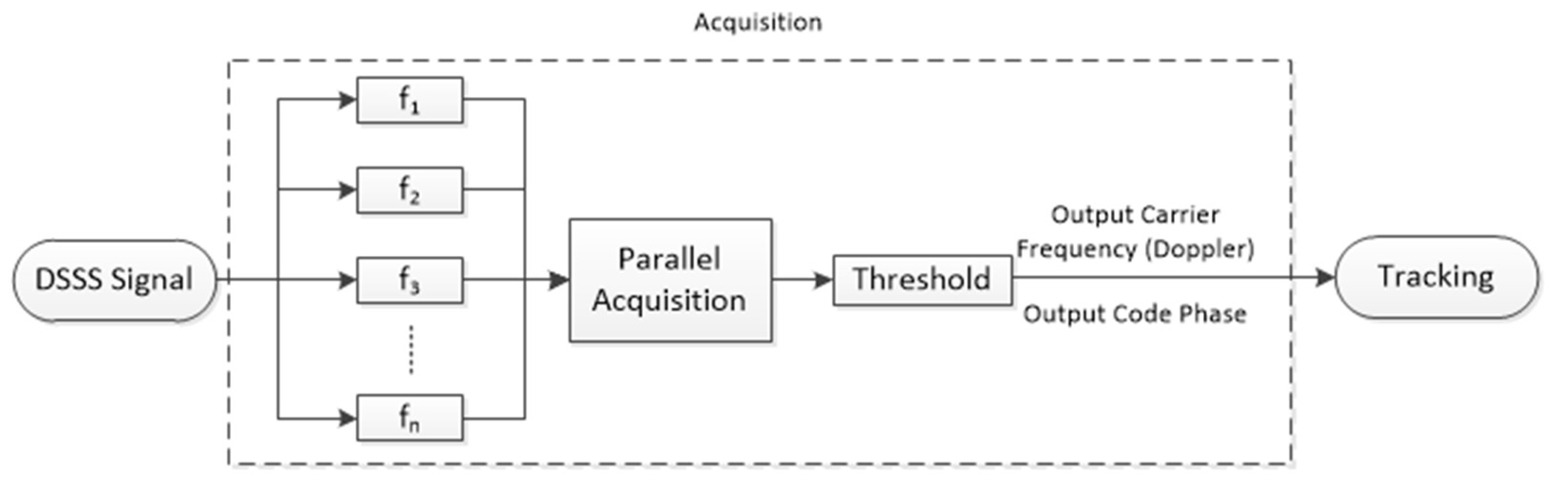
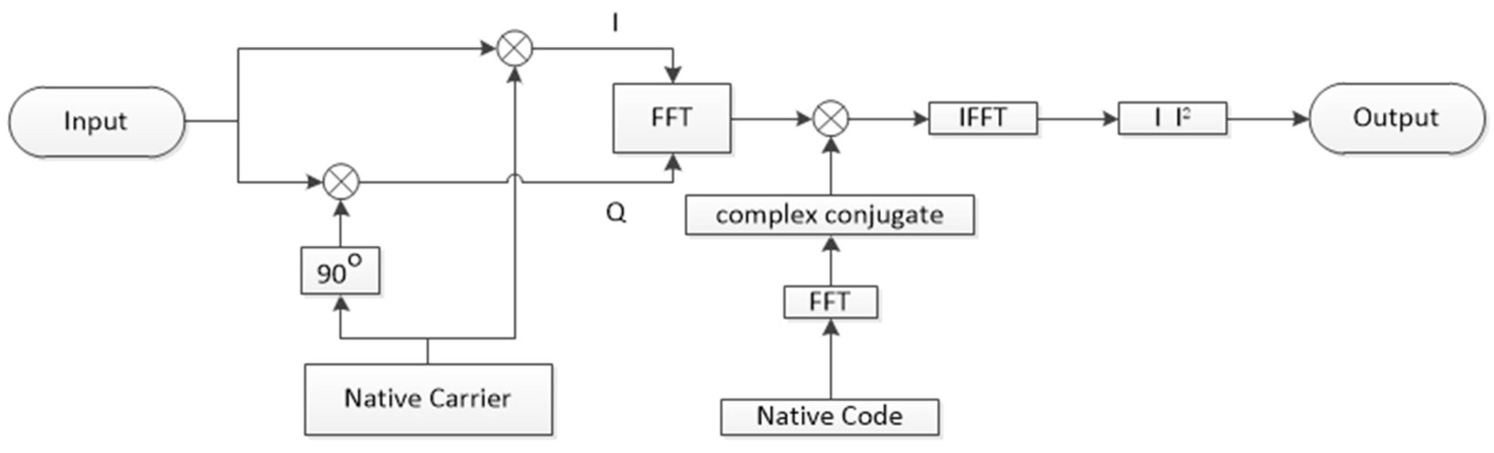
3. UWA Spread-Spectrum Signal Reception Method

3.1. UWA Signal Reception Model

The structure of the receiving system is designed to achieve stable reception of the UWA spread-spectrum signal, as illustrated in Figure 4. The carrier frequency and code phase are detected by the acquisition process [27].

To adapt to the low-frequency characteristics of the underwater acoustic (UWA) channel, a carrier frequency of approximately 20 kHz is used [28], and the Composite Spread Spectrum Sequence (CCOS) is applied for data code modulation.

The generation of CCOS requires a bitwise exclusive OR operation between a Walsh sequence and a logistic chaotic sequence of the same bit length. The structure of the CCOS generator is illustrated in Figure 5, where process L represents the mapping equation of the logistic chaotic sequence [29].

The acquisition process provides a rough estimation of the carrier frequency and code phase, enabling the determination of the Doppler shift and code delay for subsequent tracking. To ensure continuous signal tracking, the receiver must generate a spread-spectrum sequence and carrier signal that accurately match the received signal while keeping the Doppler shift error within half of the frequency search step. Consequently, enhancing acquisition speed has become a critical focus, especially in scenarios where high acquisition precision is not required.

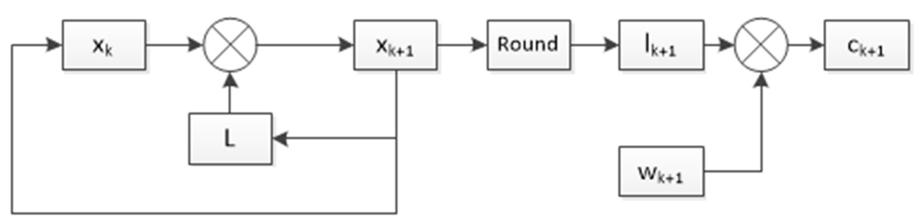
3.2. Acquisition Algorithm

The parallel algorithm based on Fast Fourier Transform (FFT) utilizes digital signal processing to significantly reduce computational complexity and acquisition time by replacing the traditional correlator for performing correlation operations [30]. This approach can be integrated into the acquisition process of UWA spread-spectrum signals. The structure of this algorithm is shown in Figure 6.

First, to extract the in-phase (I) and quadrature (Q) signals, the received signal is multiplied by the carrier signal, separating it into I and Q components. Next, the FFT is applied to convert the I and Q signals into the frequency domain. The same transformation is performed on the complex conjugate of the native spread-spectrum sequence. Finally, the two FFT results are multiplied to facilitate signal processing. The input of the FFT calculator can be written as

$$I+jQ={\displaystyle \sum _{i=1}^{L}r(k)\exp [-j(\omega d-\widehat{\omega }d)(i{T}_s)]}$$

(13)

$$\left[\begin{array}{c}{Y}_1\\ Y_2\\ ⋮\\ Y_L\end{array}\right]=FFT\left[\begin{array}{c}{r}_1\exp [-j(\omega d-\widehat{\omega }d)T_s]\\ r_2\exp [-j(\omega d-\widehat{\omega }d)2T_s]\\ ⋮\\ r_L\exp [-j(\omega d-\widehat{\omega }d)L{T}_s]\end{array}\right]$$

(14)

where r(k) represents the input of the FFT calculator, and ω_d represents the Doppler shift. The output of the FFT calculator can be written as follows:

$$\left[\begin{array}{c}{C}_1\\ C_2\\ ⋮\\ C_L\end{array}\right]=FFT*\left[\begin{array}{c}{C}_{PN1}\\ C_{PN2}\\ ⋮\\ C_{PNL}\end{array}\right]$$

(15)

FFT* represents the complex conjugate of FFT, and the output of the FFT* calculator can be expressed as follows:

$$\left[\begin{array}{c}R(1,\widehat{\omega }d)\\ R(2,\widehat{\omega }d)\\ ⋮\\ R(L-\widehat{\omega }d)\end{array}\right]=IFFT\left[\begin{array}{c}{C}_1{Y}_1\\ C_2{Y}_2\\ ⋮\\ C_L{Y}_L\end{array}\right]$$

(16)

Finally, an acquisition threshold is established and compared with the cyclic correlation values for all code phases using the inverse fast Fourier transform (IFFT). If the correlation peak exceeds the threshold, acquisition is considered successful. The correlation, which serves as the output of the IFFT calculator, is represented by Equation (14). If the peak correlation value surpasses the threshold, the acquisition process is successfully completed.

4. Simulation Results

4.1. Description of BELLHOP

The BELLHOP ray acoustic model was utilized to simulate the UWA channel environment [31,32]. This model employs Gaussian beam ray tracing theory to compute sound field parameters in horizontal and inhomogeneous environments. It is particularly suitable for addressing high-frequency variations in horizontal sound fields, where alternative methods such as normal mode theory, the wavenumber integral method, and the parabolic model may be less effective. The fundamental principle of Gaussian beam ray tracing is to associate each sound ray with a Gaussian intensity distribution.

In this study, the BELLHOP was used to construct the UWA channel model. Prior to simulation, various underwater environmental parameters were defined, including channel geometry, sound velocity profile, submarine topography, interface reflection loss and an ocean current speed model [33]. Based on this input, key channel characteristics, such as the number of multipaths, incident angles, signal amplitude, and time delays, were computed. These parameters are essential for deriving the impulse response of the system, which is the primary objective of employing the BELLHOP ray acoustic model. A schematic representation of the BELLHOP model is provided in Figure 7.

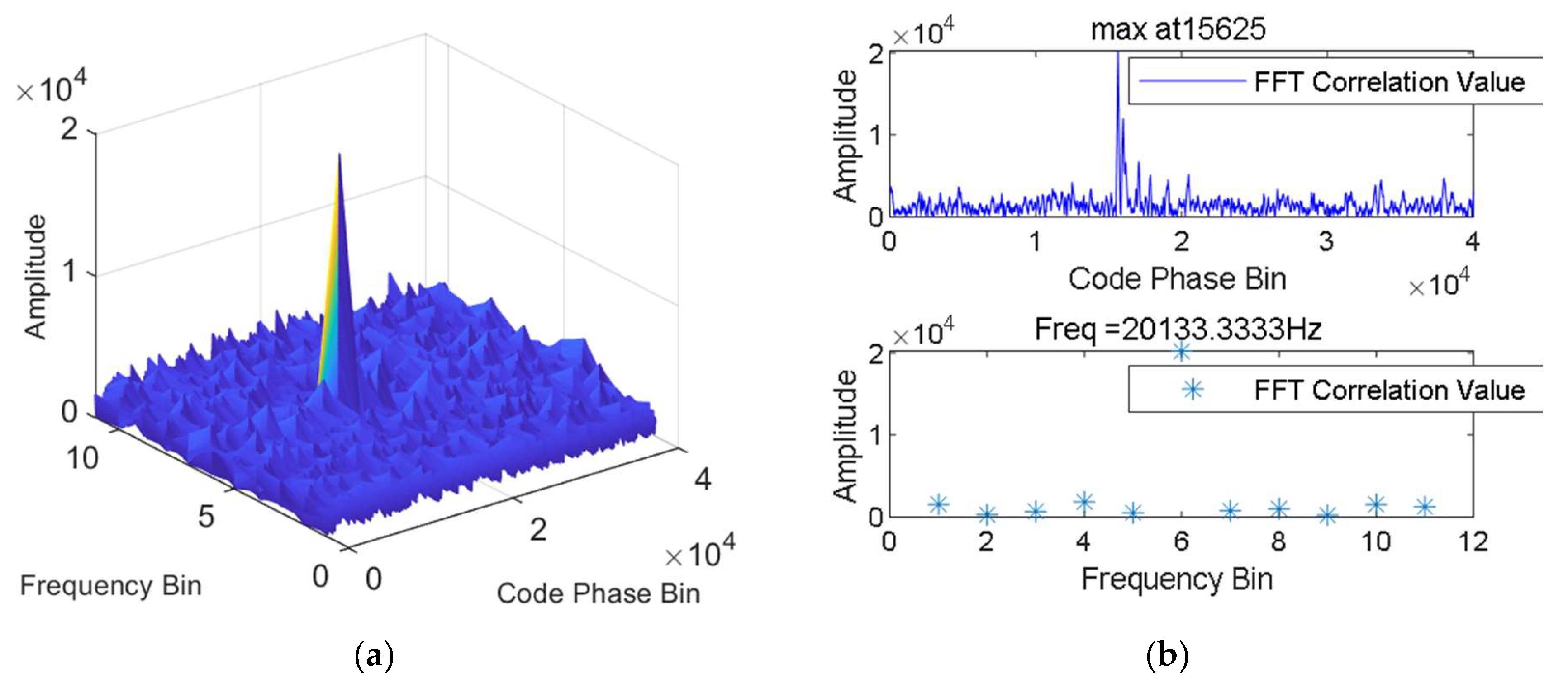
4.2. Acquisition of Underwater Acoustic Spread-Spectrum Signal

Before the acquisition process, specific parameters for frequency searching needed to be defined. Given that the intermediate frequency (IF) was 20 kHz, the frequency search range was set between 19.5 kHz and 20.5 kHz. The frequency search step was set to 100 Hz. Figure 8 illustrates the acquisition results under a signal-to-noise ratio (SNR) of −10 dB, with a CCOS length of 256 bits.

As indicated in Figure 8, the acquisition results reveal a distinct peak, which signifies that the spread-spectrum signal has been successfully received. The ratio between the first peak and second peak is 1.58. The code phase received is 15,625, and the Doppler shift is 133.33 Hz, which is 3.04 Hz greater than the theoretical value and less than half of the frequency-search element, indicating successful acquisition. The error compared to the theoretical value is mainly attributed to the error of relative speed caused by ocean currents.

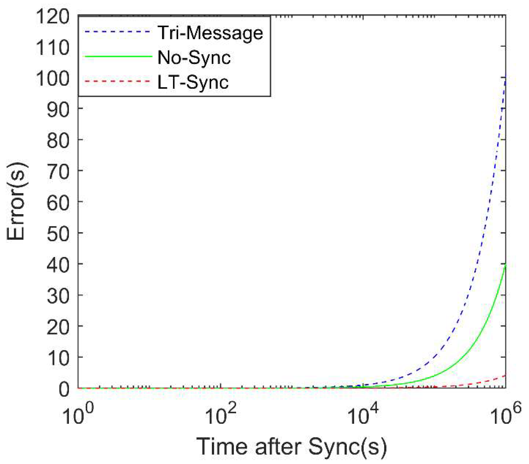
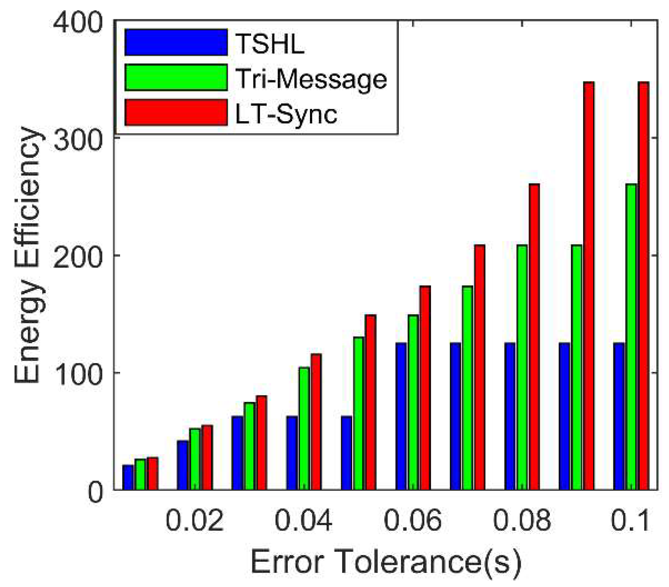
4.3. Performance Evaluation of LT-Sync

In order to validate the scheme proposed in this paper, LT-Sync is evaluated in the simulation environment developed with the underwater node distribution scheme shown in Figure 3. Because there is no scheme for high-speed mobile UWASN and Tri-Message has been the only lightweight time synchronization scheme applied in an UWA environment, we compare the performances of LT-Sync, Tri-Message and a blank control group (No-Sync) under the same simulation environment. All timestamps are obtained from the MAC layer, and other parameters are listed in

Table 1. Parameter setting.

Parameters	Values
Original distance	1485 m
Speed of unsynchronized node	15 m/s
Speed of sound	1500 m/s
Frequency of synchronization signal	100 Hz
Clock skew	40 ppm
Clock offset	80 µs
Interval between two messages	5 s
Clock granularity	1 µs
Reception jitter	15 µs
Number of messages (TSHL)	25

:

Figure 9 displays how the synchronization errors increase after time synchronization is completed with these schemes. From this figure, we can see that LT-Sync produces only about 5 s error after 10⁶ s of synchronization, outperforming Tri-Message and No-Sync. This is because LT-Sync utilizes the Doppler shift to estimate the speed of the unsynchronized node and obtain high-accuracy propagation delay estimates. On the contrary, the clock error corrected by Tri-Message is even greater than that for No-Sync, which means that it estimates clock skew incorrectly. This is because Tri-Message considers that the three propagation delays are equal, and it ignores the relative speed of the unsynchronized node.

The performances of the three schemes after 10 s of synchronization with different initial skews are shown in Figure 10. The simulation is performed with the range of the initial skew from 10⁻⁴ to 10⁻⁵ ppm. As can be seen from this figure, LT-Sync has consistent performance across different skews, and it obviously outperforms Tri-Message and No-Sync when there is a large initial skew. On the contrary, Tri-Message incorrectly estimates clock skew because it cannot obtain accurate propagation delays.

Due to the effect of the speed of the unsynchronized node during the process of estimating propagation delays, the performance of LT-Sync under different speeds of the unsynchronized node needs to be evaluated. The range of speed considered is from 11 m/s to 20 m/s. The effect of different speeds of the unsynchronized node on the accuracy of clock skew estimation is shown in Figure 11. LT-Sync reduces the cumulative error of clock skew in high-speed mobile UWASNs when compared to No-Sync by estimating the speed of the unsynchronized node. Tri-Message assumes that the three propagation delays are equal, so the higher the speed of the unsynchronized node, the larger the error in propagation delay estimation. In this case, the estimation error of the clock skew increases with the speed of the unsynchronized node.

The energy efficiency [15] of various synchronization schemes is compared in Figure 12. The energy consumed by the data processing is negligible compared to the energy consumed by the sending and receiving process of packets; hence, only the latter needs to be studied. The formula for energy efficiency is as follows [34]:

$$\rho ={\displaystyle \frac{\vartheta }{\kappa \mu \gamma }}$$

(17)

In this equation, $\vartheta$ is set to 10⁵ s, which denotes the period of time after synchronization is complete. $\mu$ is the number of messages used in the synchronization process. For TSHL, $\mu$ is set to 25, and for Tri-Message and LT-Sync, it is set to 3. $\gamma$ represents the packet size, which is set to 32 bytes. $\kappa$ denotes the number of re-synchronizations required within a certain duration of $\vartheta$, which keeps synchronization error below a certain clock error tolerance $e$, and it is expressed by (18). In the simulation, $e$ is set from 0.01 to 0.1.

$$\kappa ={\displaystyle \frac{\vartheta }{\left(\frac{\widehat{\alpha }e+\left(\widehat{\beta }-\beta \right)}{\alpha -\widehat{\alpha }}\right)}}$$

(18)

From (17) and (18), it can be seen that the energy efficiency of the scheme is determined by the estimation accuracy of clock parameters and the number of packets exchanged. LT-Sync has higher clock drift rate estimation accuracy compared to Tri-Message and TSHL, so it performs fewer synchronizations and has higher energy efficiency.

5. Conclusions

In this paper, we presented LT-Sync, a lightweight time synchronization scheme for high-speed mobile UWASNs. It is the only scheme for high-speed mobile UWASNs with high energy efficiency, and compared to Tri-Message, this scheme utilizes the Doppler shift to estimate the speed of the unsynchronized node and then derives the time delay. It can achieve high accuracy in time synchronization even when the node is moving at high speed in specific underwater conditions. LT-Sync produces only about 5 s error after 10⁶ s of synchronization, and it has consistent performance across different skews and speeds. In addition, it has better energy efficiency than Tri-Message and TSHL. Our simulation results based on the spread-spectrum method with BELLHOP show that this new approach can achieve high accuracy with low message overhead.

However, LT-Sync has some limitations, as follows:

(1)

The approximation from (9) creates a systematic error. Although it does not have a huge impact on synchronization accuracy, as the synchronization interval increases, this error may increase, too.

(2)

The way the unsynchronized node moves is specifically designed. When synchronization starts, the direction and speed of the unsynchronized node will not change until synchronization ends. It is hard to constrain movement of nodes in large-scale UWASNs.

In the future, we will continue to explore other lightweight schemes to improve the accuracy of synchronization and reduce the message overhead for mobile UWASNs. For example, the direction and speed of the unsynchronized node can be changed in real-world experiments, and the error caused by (9) may be revised by a more efficient way of obtaining time delay. And there may be a more accurate method to estimate the speed by the Doppler shift, which can be used for obtaining the variation in relative speed caused by ocean currents in both shallow-water and deep-water environments. In addition, we also plan to study convergence time and overall energy consumption of large-scale, high-speed mobile UWASNs with LT-Sync, because some evaluations may change due to increasing network density.

References

1. Liu, J.; Wang, Z.H.; Cui, J.H.; Zhou, S.L.; Yang, B. A Joint Time Synchronization and Localization Design for Mobile Underwater Sensor Networks. IEEE Trans. Mob. Comput. 2016, 15, 530–543. [Google Scholar] [CrossRef]
2. Luo, H.J.; Wu, K.S.; Ruby, R.; Hong, F.; Guo, Z.W.; Ni, L.M. Simulation and Experimentation Platforms for Underwater Acoustic Sensor Networks: Advancements and Challenges. ACM Comput. Surv. 2017, 50, 1–44. [Google Scholar] [CrossRef]
3. Vermeij, A.; Munafò, A. A Robust, Opportunistic Clock Synchronization Algorithm for Ad Hoc Underwater Acoustic Networks. IEEE J. Ocean. Eng. 2015, 40, 841–852. [Google Scholar] [CrossRef]
4. Tuna, G.; Gungor, V.C. A survey on deployment techniques, localization algorithms, and research challenges for underwater acoustic sensor networks. Int. J. Commun. Syst. 2017, 30, e3350. [Google Scholar] [CrossRef]
5. Gong, Z.J.; Li, C.; Jiang, F. AUV-Aided Joint Localization and Time Synchronization for Underwater Acoustic Sensor Networks. IEEE Signal Process. Lett. 2018, 25, 477–481. [Google Scholar] [CrossRef]
6. Gardner, A.T.; Collins, J.A. A Second Look at Chip Scale Atomic Clocks for Long Term Precision Timing Four Years in the Field. In Proceedings of the MTS/IEEE Oceans Conference, Monterey, CA, USA, 19–23 September 2016. [Google Scholar]
7. Elson, J.; Girod, L.; Estrin, D. Fine-grained network time synchronization using reference broadcasts. In Proceedings of the 5th Symposium on Operation Systems Design and Implementation (OSDI 02), Boston, MA, USA, 9–11 December 2002; pp. 147–163. [Google Scholar]
8. Ganeriwal, S.; Kumar, R.; Srivastava, M.B. Timing-sync protocol for sensor networks. In Proceedings of the 1st International Conference on Embedded Networked Sensor Systems, Los Angeles, CA, USA, 5–7 November 2003. [Google Scholar]
9. Maróti, M.; Kusy, B.; Simon, G.; Lédeczi, Á. The flooding time synchronization protocol. In Proceedings of the 2nd International Conference on Embedded Network Sensor Systems, Baltimore, MD, USA, 3–5 November 2004. [Google Scholar]
10. Syed, A.A.; Heidemann, J. Time Synchronization for High Latency acoustic networks. In Proceedings of the IEEE INFOCOM 2006 Conference/25th IEEE International Conference on Computer Communications, Barcelona, Spain, 23–29 April 2006; pp. 892–903. [Google Scholar]
11. Chirdchoo, N.; Soh, W.-S.; Chua, K.C. MU-Sync: A time synchronization protocol for underwater mobile networks. In Proceedings of the 3rd International Workshop on Underwater Networks, San Francisco, CA, USA, 15 September 2008; pp. 35–42. [Google Scholar]
12. Lu, F.; Mirza, D.; Schurgers, C. D-sync: Doppler-based time synchronization for mobile underwater sensor networks. In Proceedings of the 5th International Workshop on Underwater Networks, Woods Hole, MA, USA, 30 September–1 October 2010. Article 3. [Google Scholar]
13. Liu, J.; Wang, Z.H.; Zuba, M.; Peng, Z.; Cui, J.H.; Zhou, S.L. DA-Sync: A Doppler-Assisted Time-Synchronization Scheme for Mobile Underwater Sensor Networks. IEEE Trans. Mob. Comput. 2014, 13, 582–595. [Google Scholar] [CrossRef]
14. Zhou, F.; Wang, Q.; Nie, D.; Qiao, G. DE-Sync: A Doppler-Enhanced Time Synchronization for Mobile Underwater Sensor Networks. Sensors 2018, 18, 1710. [Google Scholar] [CrossRef] [PubMed]
15. Zhou, F.; Wang, Q.; Han, G.J.; Qiao, G.; Sun, Z.X.; Niaz, A. APE-Sync: An Adaptive Power Efficient Time Synchronization for Mobile Underwater Sensor Networks. IEEE Access 2019, 7, 52379–52389. [Google Scholar] [CrossRef]
16. Tian, C.; Jiang, H.B.; Liu, X.; Wang, X.B.; Liu, W.Y.; Wang, Y. Tri-Message: A Lightweight Time Synchronization Protocol for High Latency and Resource-Constrained Networks. In Proceedings of the 2009 IEEE International Conference on Communications (ICC 2009), Dresden, Germany, 14–18 June 2009; pp. 1–5. [Google Scholar]
17. Ouyang, Y.J.; Han, Y.F.; Wang, Z.Y.; He, Y.F. Underwater Network Time Synchronization Method Based on Probabilistic Graphical Models. J. Mar. Sci. Eng. 2024, 12, 2079. [Google Scholar] [CrossRef]
18. Sun, D.J.; Ouyang, Y.J.; Han, Y.F. DC-Sync: A Doppler-Compensation Time-Synchronization Scheme for Complex Mobile Underwater Sensor Networks. IEEE Access 2024, 12, 94643–94653. [Google Scholar] [CrossRef]
19. Wang, X.R.; Su, Y.S.; Fan, R. SFDM: A time-synchronization-free detection mechanism for mobile underwater acoustic sensor networks. Ocean Eng. 2024, 311, 118983. [Google Scholar] [CrossRef]
20. Zhou, F.; Zhang, W.B.; Zhang, B.S.; Nie, D.H.; Wang, Y.; Liu, B. Underwater Acoustic Spread Spectrum Communications Based on Space-Time Cluster Processing. J. Electron. Inf. Technol. 2022, 44, 2006–2013. [Google Scholar] [CrossRef]
21. Li, Y.; Liu, B.; Jia, N.; Huang, J.C.; Xiao, D.; Guo, S.M. A Study of Mapping Sequences Spread Spectrum Underwater Acoustic Communications Using Gold Codes. In Proceedings of the 15th ACM International Conference on Underwater Networks & Systems, Shenzhen, China, 23–26 November 2021. [Google Scholar]
22. Hu, Y.H.; Han, S.P.; Liu, J.B.; Zhang, Q.; Zhang, Y.H. Combination Differential Direct Sequence Spread Spectrum Algorithm for Mobile Underwater Acoustic Communication. J. Electron. Inf. Technol. 2022, 44, 2024–2034. [Google Scholar] [CrossRef]
23. Shu, X.J.; Wang, J.; Wang, H.B.; Yang, X.X. Chaotic direct sequence spread spectrum for secure underwater acoustic communication. Appl. Acoust. 2016, 104, 57–66. [Google Scholar] [CrossRef]
24. Du, P.Y.; Xiong, S.J.; Wang, C. Research on mobile spread spectrum underwater acoustic communication. In Proceedings of the IEEE International Conference on Signal Processing, Communications and Computing (ICSPCC), Dalian, China, 20–22 September 2019. [Google Scholar]
25. Lasassmeh, S.M.; Conrad, J.M. Time Synchronization in Wireless Sensor Networks: A Survey. In Proceedings of the IEEE SoutheastCon 2010 Conference on Energizing Our Future, Concord, NC, USA, 18–21 March 2010; pp. 242–245. [Google Scholar]
26. Yang, L.; Yang, L.; Ho, K.C. Moving Target Localization in Multistatic Sonar by Differential Delays and Doppler Shifts. IEEE Signal Process. Lett. 2016, 23, 1160–1164. [Google Scholar] [CrossRef]
27. Xiao, L.L.; Xuan, G.X.; Wu, Y.B. Research on an Improved Chaotic Spread Spectrum Sequence. In Proceedings of the 3rd IEEE International Conference on Cloud Computing and Big Data Analysis (ICCCBDA), Chengdu, China, 20–22 April 2018; pp. 420–423. [Google Scholar]
28. Ra, H.; Youn, C.; Kim, K. High-Reliability Underwater Acoustic Communication Using an M-ary Cyclic Spread Spectrum. Electronics 2022, 11, 1698. [Google Scholar] [CrossRef]
29. Sun, K.; Zhou, J.; Mou, J. Design and Performance Analysis of Multi-user Chaotic Sequence Spread-Spectrum Communication System. J. Electron. Inf. Technol. 2007, 29, 2436–2440. [Google Scholar]
30. Kim, B.; Kong, S.H. Design of FFT-Based TDCC for GNSS Acquisition. IEEE Trans. Wirel. Commun. 2014, 13, 2798–2808. [Google Scholar] [CrossRef]
31. Narykov, A.; Wright, M.; García-Fernández, A.F.; Maskell, S.; Ralph, J.F. Poisson multi-Bernoulli mixture filtering with an active sonar using BELLHOP simulation. In Proceedings of the 25th International Conference of Information Fusion (FUSION), Linkoping, Sweden, 4–7 July 2022. [Google Scholar]
32. Ghafoor, H.; Noh, Y.; Koo, I. OFDM-based spectrum-aware routing in underwater cognitive acoustic networks. IET Commun. 2017, 11, 2613–2620. [Google Scholar] [CrossRef]
33. Lin, J.Y.; Feng, G.S.; Wen, X.X.; Wang, H.Q.; Lv, H.W.; Zhao, Q.; Han, J.Z. MM-sync: A Mobility Built-in Model Based Time Synchronization Approach for Underwater Sensor Networks. In Proceedings of the 2016 IEEE International Conferences on Big Data and Cloud Computing (BDCloud), Social Computing and Networking (SocialCom), Sustainable Computing and Communications (SustainCom) (BDCloud-SocialCom-SustainCom), Atlanta, GA, USA, 8–10 October 2016; pp. 338–345. [Google Scholar]
34. Liu, J.; Wang, Z.H.; Peng, Z.; Zuba, M.; Cui, J.H.; Zhou, S.L. TSMU: A Time Synchronization Scheme for Mobile Underwater Sensor Networks. In Proceedings of the 54th Annual IEEE Global Telecommunications Conference (GLOBECOM), Houston, TX, USA, 5–9 December 2011. [Google Scholar]
Figure 1. Sender–receiver two-way synchronization.
Jmse 13 00528 g001
Figure 2. LT-Sync message exchange scheme.
Jmse 13 00528 g002
Figure 3. Underwater node distribution scheme of LT-Sync.
Jmse 13 00528 g003
Figure 4. Structure of the receiving system.
Jmse 13 00528 g004
Figure 5. Structure of CCOS generator.
Jmse 13 00528 g005
Figure 6. Structure of the parallel algorithm based on FFT.
Jmse 13 00528 g006
Figure 7. Schematic of the BELLHOP model.
Jmse 13 00528 g007
Figure 8. (a) Three-dimensional acquisition results; (b) Acquisition results with more details.
Jmse 13 00528 g008
Figure 9. Clock error vs. time after synchronization.
Jmse 13 00528 g009
Figure 10. Performance with initial skew.
Jmse 13 00528 g010
Figure 11. Performance with relative speed.
Jmse 13 00528 g011
Figure 12. Energy efficiency vs. error tolerance.
Jmse 13 00528 g012