Cooperative Formation Control of Multiple Ships with Time Delay Conditions

Abstract

The cooperative control of multiple autonomous surface vehicles (ASVs) is a critical area of research due to its significant applications in maritime operations, such as search and rescue and environmental monitoring. However, challenges such as communication delays and dynamic topologies often hinder stable cooperative control in practical scenarios. This study addresses these challenges by developing a formation control method based on consensus theory, focusing on both formation control and time delay. First, a simplified ASV characteristic model is established, and a basic consensus control algorithm is designed and analyzed for stability, considering different communication topologies. Then, to handle delays, the formation control method is extended, and the stability of the revised algorithm is rigorously proven using the Lyapunov function. Simulation results demonstrate that the proposed control strategy effectively maintains formations, even in the presence of communication delays. In the end, comparative simulations are carried out to demonstrate the effectiveness and robustness of the proposed controller. Simulation results demonstrate that the proposed control strategy effectively maintains formations, even in the presence of communication delays, with a convergence time of approximately 100 s and a formation error stabilizing at around 7 m. This research lays a foundation for more reliable cooperative control systems for ships, with potential applications in a variety of maritime and autonomous systems.

1. Introduction

The collaboration of vessels in waterway transportation systems offers many benefits. First, it can enhance the safety of waterway transport through communication between vessels. Such communication provides additional information, such as data about objects that sensors cannot detect and the intentions of other vessels. This information helps vessel operators collaborate and take effective actions [1]. Second, collaboration can improve transportation efficiency [2]. For example, vessels can coordinate their navigation plans to avoid congestion at ports and locks [3]. Additionally, by integrating route planning with infrastructure scheduling, vessels can adjust their speeds to reach their destinations on time, optimizing the use of infrastructure resources [4]. Finally, collaboration allows a group of vessels to perform tasks more effectively, such as search and rescue, ocean sampling, and hydrographic surveys [5]. Therefore, optimizing waterway transport performance requires not only the automation of individual vessels but also collaboration between them.

Given the advantages of vessel cooperation, recent years have seen increasing research on various cooperative methods [6,7]. For cooperative methods, communication is the premise of formation control. However, communication delays are inevitable in reality. Delays in communication among formation members may lead to inaccuracies in the status of the ship and even lead to invalidation of the whole operation. Thus, communication delays are crucial in ship formation control.

Cooperative control of multiple autonomous surface vehicles has become a crucial area of research due to its potential to revolutionize various maritime applications, including search-and-rescue operations, environmental monitoring, and autonomous transportation [8]. These applications benefit from the cooperative capabilities of multiple ships, leading to enhanced efficiency, safety, and adaptability in dynamic maritime environments. However, the practical implementation of cooperative control for ships is often hindered by challenges such as communication delays, which significantly impact the stability and performance of cooperative behaviors, especially in real-time operations.

This study addresses the challenges of formation control by proposing a novel strategy based on consensus theory. The core methodology involves the design and analysis of a simplified autonomous surface vehicle model, in which a basic consensus algorithm is employed to ensure the stability of formation control under varying communication topologies. Building on this approach, this study also accounts for communication delays, a common issue in practical scenarios, and adapts the formation control method accordingly. The stability of the revised control algorithm is rigorously validated using Lyapunov’s stability theory, providing a solid theoretical foundation for its reliability. Our contributions are as follows:

(1)

Development of a consensus-based formation control algorithm capable of handling various communication topologies, ensuring stability in dynamic environments.

(2)

Extension of the control strategy to accommodate communication delays, with rigorous proof of its stability through Lyapunov’s stability theory.

This article is organized as follows. In Section 1, the introduction presents the importance of cooperative control for ships and outlines the research objectives and contributions of this study. Section 2 defines the core challenges of communication delays and dynamic topologies in multi-ASV coordination and formulates the problem to be addressed. Section 3 discusses the development of a consensus-based formation control strategy for ships, designed to handle communication delays and dynamic topologies. The proposed formation control strategy is verified through simulations in Section 4. Section 5 summarizes the findings and discusses the implications and potential future research directions.

2. Literature Review

Formation control in multi-agent systems, especially for autonomous surface vehicles (ASVs), is crucial for tasks like navigation and coordination in dynamic environments. Several key approaches have shaped the field, focusing on decentralized control and stability. Jadbabaie et al. introduced the nearest neighbor rules for agent coordination, enabling decentralized consensus and stable formations without a central controller [9]. Chung et al. highlighted the challenges of aerial swarm coordination, underscoring the need for adaptive strategies in complex environments [10]. Bunic and Bogdan’s potential-function-based approach ensures formation stability and collision avoidance in 3D space [11]. Chang et al. also contributed with algorithms for collision avoidance, vital for maintaining safe formations in high-density environments [12]. Do’s local potential functions allow for dynamic position adjustments while avoiding obstacles [13]. Anh et al. advanced this by combining rotational and repulsive forces for better obstacle avoidance and formation stability [14]. Optimization-based methods, such as those explored by Piet et al., offer valuable extensions by improving formation efficiency in constrained environments [15].

In recent years, several studies have further expanded the field. For instance, a study on multi-agent systems under external communication disturbances developed new control strategies for formation stability in the presence of unreliable communication [16]. Another work focused on formation control in directed topologies, providing a comprehensive framework for the stability of multi-agent systems [17]. Research on uncertain multi-agent systems addressed formation control under nonlinear constraints, integrating control barrier functions to ensure both safety and stability [18]. A recent paper also explored collision avoidance in multi-agent systems using consensus mechanisms, demonstrating effective formation control and collision avoidance in multi-agent systems [19]. Additionally, a study on discrete-time linear multi-agent systems proposed a control method based on stress matrices, addressing formation stability in both static and dynamic leader scenarios [20]. Another significant contribution is from a neural-network-based approach, which handles uncertainty in nonlinear multi-agent systems, enhancing cooperative formation control [21]. These studies provide the foundation for robust formation control methods. Our work extends these principles by developing a consensus-based algorithm that addresses the unique challenges of communication delays and dynamic topologies in ASV formations.

Many studies have focused on addressing the formation control problem in the presence of communication delays in ASVs, AUVs (Autonomous Underwater Vehicles), and UAVs (Unmanned Aerial Vehicles). Broadly, the existing approaches can be categorized into three main types: data-driven, observer-based, and event-triggered methods, as outlined in

Table 1. Literature review.

Research Article	Type of Vehicles			Number of Vehicles				Communication Constraints		Method
	ASV	AUV	UAV	3	4	5	6	Time-Delay	Packet Dropouts
[22]	●			●				●	●	Auto-regressive model
[23]	●			●				●		Proportional–integral (PI) predictive control
[24]	●				●			●		RBF neural networks
[25]	●						●	●		Rational approximation, based on the Hermite–Feje’r tangential interpolation condition
[26]	●						●	●		Luenberger observer
[27]	●				●			●		Radial basis function (RBF) neural networks, event-triggered
[28]	●						●	●		Consensus theory, adaptive control
[29]		●				●		●		Consensus theory
[30]		●				●		●	●	Consensus theory
[31]		●				●		●		Robust control, observer
[32]			●	●				●		Consensus theory
[33]			●		●			●	●	Consensus theory

The ● represents the objects (including the values of aircraft type, quantity, and communication constraints) studied in the paper.

.

Data-driven approaches primarily aim to develop models that predict communication latency or the states of multi-agent systems at each time step based on historical communication data. Common techniques in this category include auto-regressive models [22], PID control [23], emerging artificial intelligence models [24], and function approximation [25]. These methods are heavily dependent on historical data but can be computationally expensive and are prone to overfitting, especially when large datasets are required for model development.

Observer-based methods involve designing state observers or estimators to estimate the states of neighboring agents in the system. Notable observer models include high-gain observers [26], predictive state observers [27], and Luenberger observers [28]. Despite their strengths, these methods are often challenged by issues related to parameter selection and tuning, and they tend to be sensitive to external disturbances or noise.

Event-triggered methods adjust the communication topology dynamically when communication delays or bandwidth usage exceed predefined thresholds. These strategies often depend on measurable control variables such as rudder angles [29] or the current system state. Event-triggered mechanisms are frequently combined with other approaches, such as neural networks (NNs) [30], to reduce the communication burden among formation members. In addition to the methods mentioned above, consensus-based formation control algorithms have successfully addressed the delay problem due their convenient design [31].

Problems involving consensus-based formation control whilst considering delay have been applied and validated on various intelligent transportation platforms, including underwater [32,33,34] and air vehicles [35,36], though their application in the maritime field remains relatively limited.

On the other hand, current research classifies formation control methods into three primary categories based on formation structure [37]. The leader–follower approach designates one vessel as the leader, which follows a desired trajectory, while the followers adjust their positions relative to the leader using predefined offsets. The behavioral approach assigns different weights to various desired behaviors, such as clustering and formation maintenance, to guide the control process [38]. The virtual structure approach treats the entire formation as a single virtual entity, with the motion of individual vessels governed by the movement of this virtual structure. Formation control focuses on guiding a group of vessels to achieve a specific geometric configuration and follow a predefined path [39]. The majority of research in vessel formation control adopts one of three primary strategies: the leader–follower framework [40], the behavioral approach, or the virtual structure method. These approaches consider vessel-specific characteristics and environmental disturbances, ensuring adaptability to varying operational conditions [41,42,43].

Despite the extensive research on these methods, several critical gaps remain in the literature. Firstly, most existing methods either ignore or only partially account for the impact of communication delays on the stability of multi-agent systems. In maritime applications, where delays are often caused by long communication distances or limited bandwidth, effective compensation for delays is essential to maintaining system stability. Secondly, many studies assume a static communication topology, but in practice, the topology of communication links can change dynamically due to the motion of agents. Methods that can adapt to changing communication topologies while maintaining stable formation control are still lacking.

3. Problem Statement and Formulation

This section addresses the key challenges and formulations necessary for the cooperative control of autonomous surface vehicles in a formation.

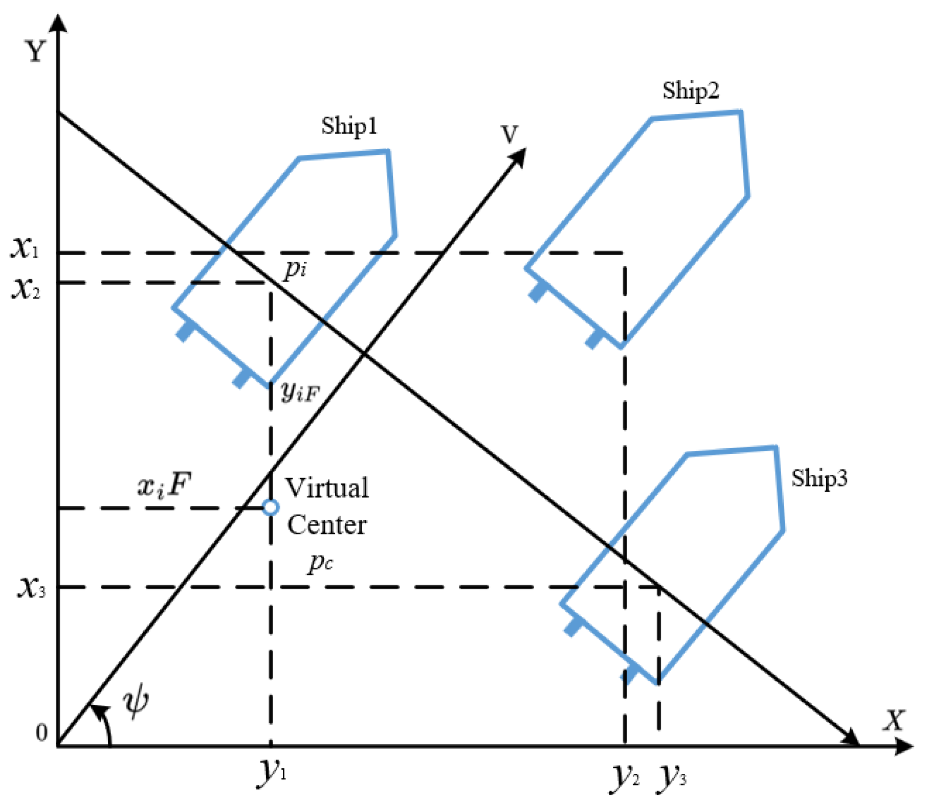
3.1. Formation Matrix Description for Ship Formation

In designing formation control strategies, a matrix capable of describing the ASV formation structure is required. This matrix enables ships positioned at different locations and with varying initial states to converge with the desired formation through control strategies, ensuring that their states become consistent. In real-world scenarios, the formation structure of ships is determined based on the tasks to be executed. Selecting an appropriate formation structure contributes to improved formation stability and enhanced cooperative capabilities.

The formation description method, as shown in Figure 1, directly projects the desired relative distances between the ships and the virtual center of the formation onto the coordinate axes. In this figure, we present a method for describing the formation of autonomous surface vehicles (ASVs) in a two-dimensional plane. The desired relative distances between the ASVs and the virtual center of the formation are projected onto the coordinate axes, simplifying the geometric relationships between the vehicles. Specifically, the virtual center serves as the reference point, and the relative positions of the ships are described in terms of their distance from this center. This approach allows for a straightforward representation of the formation, making it easier to design and implement control strategies. The cooperative variables, including position, velocity, and orientation angle, are key to achieving consensus in the formation control algorithm. These variables are synchronized among the ships to maintain the desired formation and ensure stability. This approach uses the direction coordinate system to represent these projections more straightforwardly. In Figure 1, $p_c$ represents the virtual center of the formation and serves as the reference point for other vehicles. $p_i={\left[x_i,y_i\right]}^T$ denotes the spatial coordinates of ASV i. $p_{iF}={\left[x_{iF},y_{iF}\right]}^T$ represents the desired relative position between ASV i and the virtual center of the formation. In the context of formation control strategies, the information that needs to achieve consensus is referred to as cooperative variables. For example, if the desired outcome is for all ships in the formation to align their orientation angles, then the orientation angle becomes a cooperative variable.

The two-dimensional spatial coordinates of ships are first selected as cooperative variables. The control goal is to ensure that each ASV achieves the desired distance from a reference point, expressed as:

$$‖p_{ic}-p_c‖\to 0$$

(1)

where $p_{ic}=p_i-p_{iF}$. To preserve the formation, it is also necessary to ensure that the velocities and orientation angles of all ships remain consistent. These requirements are expressed as:

$$‖v_i-v_j‖\to 0,‖{\psi }_i-{\psi }_j‖\to 0$$

(2)

where $v_i$ and ${\psi }_i$ denote the linear velocity and angle of ASV i, respectively. To design an effective formation control strategy, it is essential to ensure that each ASV accurately obtains and converges to these cooperative variables, which include position, velocity, and orientation angle.

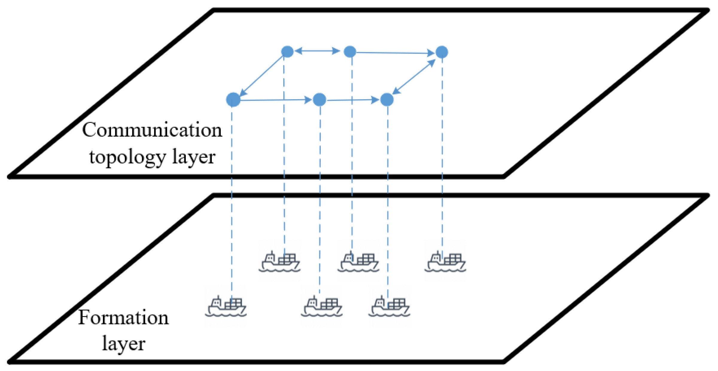
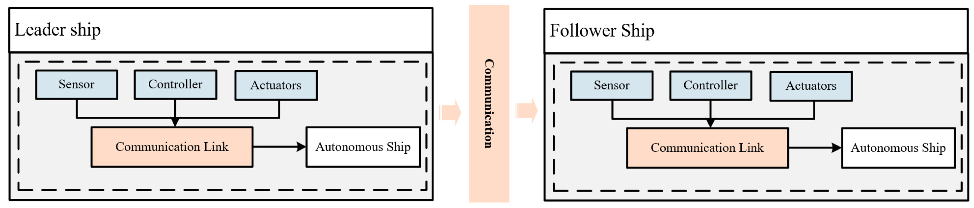
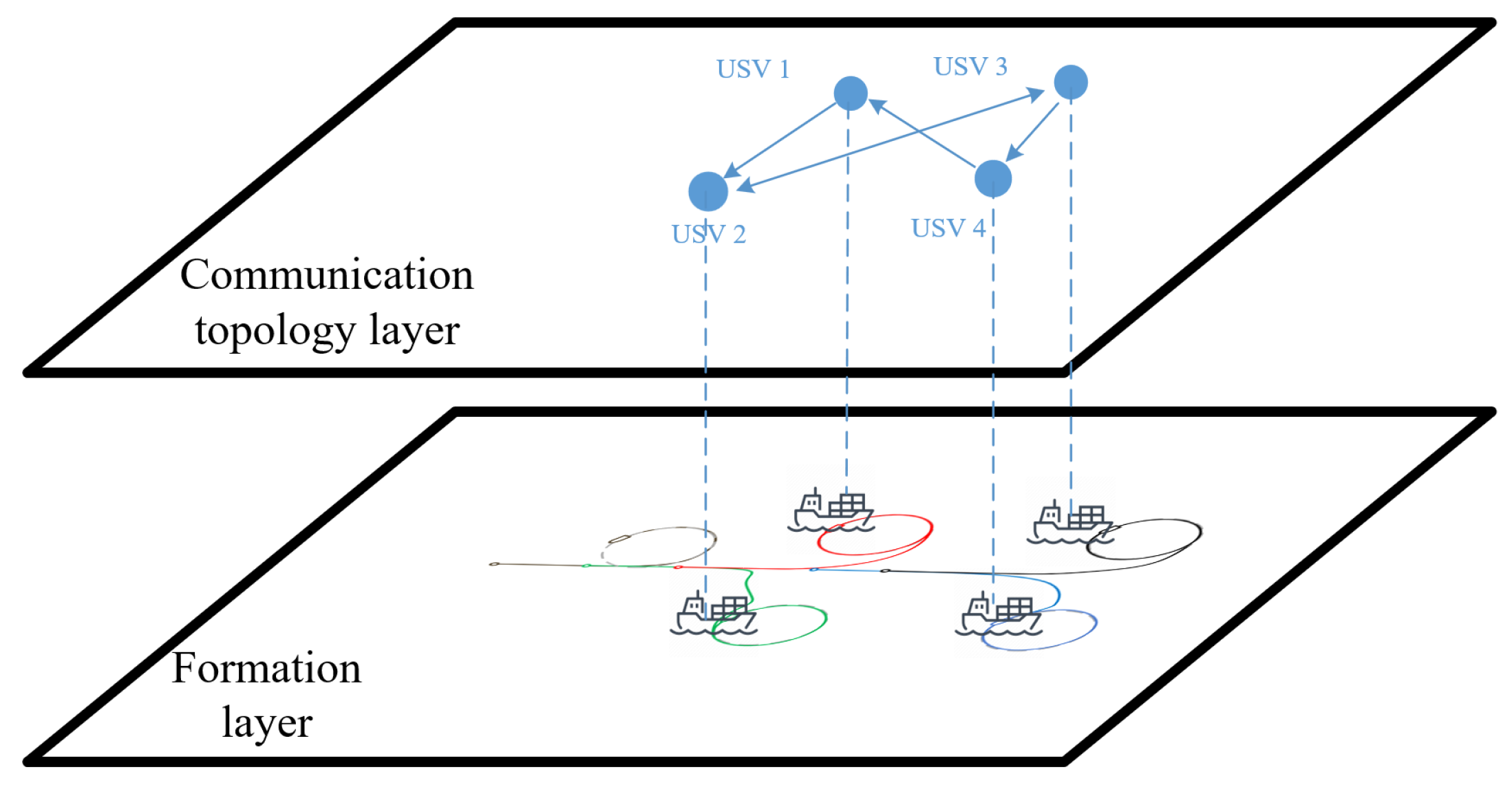
3.2. Construction of Communication Topology Models

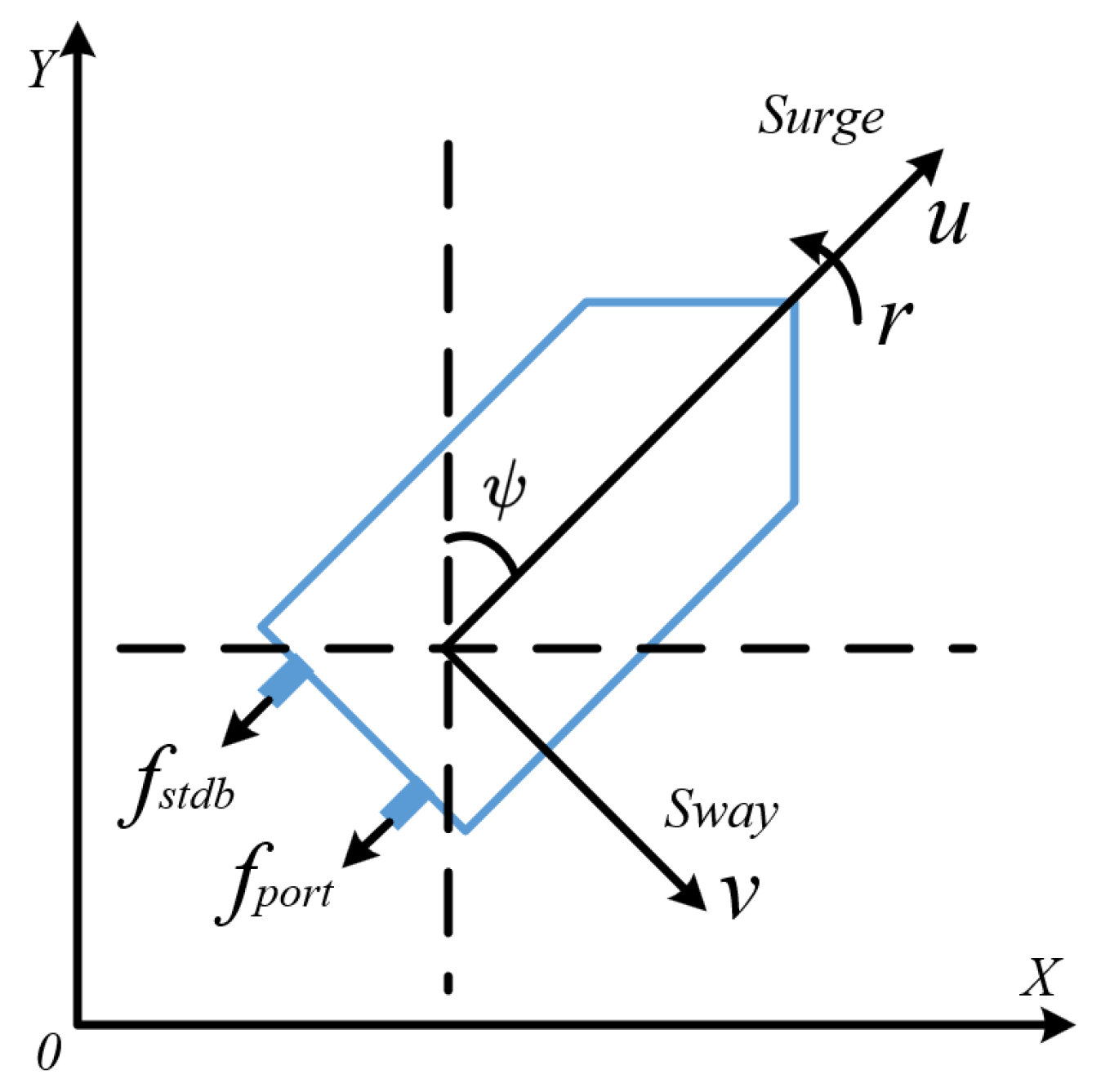
To model and control twin-propulsion ships, graph theory is utilized to establish a communication topology structure that connects individual ships, thereby forming a coordinated formation system. The following discusses the use of mathematical graph theory to describe the information exchange relationships between ships within a group.

In graph theory, graphs are divided into directed graphs and undirected graphs. A directed graph is represented as G = ($v_n$, ${\epsilon }_n$), where $v_n$ = {1, 2, …, n} is the set of nodes (representing the ships). ${\epsilon }_n$ = $v_n$ × $v_n$ is the set of edges (representing communication links between nodes). An edge (i, j) ∈ ε indicates that node j is a neighboring node of node i.

In most practical formation scenarios, directed graphs are typically used to represent the communication topology. In a directed graph, multiple nodes capable of transferring information can be connected, forming a directed path. For instance, in a directed path, information can flow from node 1 to node 4 sequentially.

Some specific communication topology structures in graph theory have significant implications for formation control of ships. During the design process, these structures are often referred to or adapted to optimize the communication topology for the formation system. By leveraging insights from graph theory, the design of robust communication structures enables efficient coordination and control of ASV formations. For a directed graph $\left(v_n,{\epsilon }_n\right)$, the adjacency matrix $A_n=\left[a_{ij}\right]\in R^{n\times n}$ is defined as follows: for any edge $(i,j)\in {\epsilon }_n$, node i can receive information from node j, and $a_{ij}>0$.

For a directed weighted graph with n n nodes, the in-degree of a certain node is defined as $d_{ii}=\sum a_{ij}$ The in-degree matrix is then $D=\mathrm{d}\mathrm{i}\mathrm{a}\mathrm{g}\left\{d_{ii}\right\}$.

The Laplacian matrix $L_n=\left[l_{ij}\right]\in R^{n\times n}$ is defined as:

$$l_{ij}=\left\{\begin{array}{c}-a_{ij}, i\ne j\\ {\sum }_{i\ne j} a_{ij}, i=j\end{array}\right.$$

(3)

Equivalently, $L_n=\left[l_{ij}\right]\in R^{n\times n}$, $L_n=D-A_n$, where $D=\left[d_{ij}\right]\in R^{n\times n}$. By the properties of the matrix, for any $(i,j)\notin {\epsilon }_n$, $l_{ij}=-a_{ij}=0$, the Laplacian matrix $L_n$ satisfies the following:

$$l_{ij}\le 0,i\ne j,{\sum }_{j=1} l_{ij}=0, i=\mathrm{1,2},\cdots n$$

(4)

The Laplacian matrix of a directed graph is asymmetric; it satisfies the property of having a simple zero eigenvalue. For the communication topology shown in Figure 2, using graph theory, we model the communication network between the ships, with nodes representing the ships and edges representing communication links. A directed graph is used to depict the flow of information, ensuring that each ship can receive and transmit data to its neighboring ships. The structure of this communication network is critical for maintaining stable formation control, as it determines how the ships share information with each other. The corresponding matrix representation is as follows:

$$A=\left[\begin{array}{c}0\hspace{0.25em}\hspace{0.25em}\hspace{0.25em}\hspace{0.25em}1\hspace{0.25em}\hspace{0.25em}\hspace{0.25em}\hspace{0.25em}0\hspace{0.25em}\hspace{0.25em}\hspace{0.25em}\hspace{0.25em}0\hspace{0.25em}\hspace{0.25em}\hspace{0.25em}\hspace{0.25em}0\hspace{0.25em}\hspace{0.25em}\hspace{0.25em}\hspace{0.25em}0\\ 1\hspace{0.25em}\hspace{0.25em}\hspace{0.25em}\hspace{0.25em}0\hspace{0.25em}\hspace{0.25em}\hspace{0.25em}\hspace{0.25em}0\hspace{0.25em}\hspace{0.25em}\hspace{0.25em}\hspace{0.25em}0\hspace{0.25em}\hspace{0.25em}\hspace{0.25em}\hspace{0.25em}0\hspace{0.25em}\hspace{0.25em}\hspace{0.25em}\hspace{0.25em}0\\ 1\hspace{0.25em}\hspace{0.25em}\hspace{0.25em}\hspace{0.25em}0\hspace{0.25em}\hspace{0.25em}\hspace{0.25em}\hspace{0.25em}0\hspace{0.25em}\hspace{0.25em}\hspace{0.25em}\hspace{0.25em}0\hspace{0.25em}\hspace{0.25em}\hspace{0.25em}\hspace{0.25em}0\hspace{0.25em}\hspace{0.25em}\hspace{0.25em}\hspace{0.25em}0\\ 0\hspace{0.25em}\hspace{0.25em}\hspace{0.25em}\hspace{0.25em}1\hspace{0.25em}\hspace{0.25em}\hspace{0.25em}\hspace{0.25em}1\hspace{0.25em}\hspace{0.25em}\hspace{0.25em}\hspace{0.25em}0\hspace{0.25em}\hspace{0.25em}\hspace{0.25em}\hspace{0.25em}0\hspace{0.25em}\hspace{0.25em}\hspace{0.25em}\hspace{0.25em}0\\ 0\hspace{0.25em}\hspace{0.25em}\hspace{0.25em}\hspace{0.25em}0\hspace{0.25em}\hspace{0.25em}\hspace{0.25em}\hspace{0.25em}1\hspace{0.25em}\hspace{0.25em}\hspace{0.25em}\hspace{0.25em}0\hspace{0.25em}\hspace{0.25em}\hspace{0.25em}\hspace{0.25em}0\hspace{0.25em}\hspace{0.25em}\hspace{0.25em}\hspace{0.25em}1\\ 0\hspace{0.25em}\hspace{0.25em}\hspace{0.25em}\hspace{0.25em}0\hspace{0.25em}\hspace{0.25em}\hspace{0.25em}\hspace{0.25em}0\hspace{0.25em}\hspace{0.25em}\hspace{0.25em}\hspace{0.25em}1\hspace{0.25em}\hspace{0.25em}\hspace{0.25em}\hspace{0.25em}1\hspace{0.25em}\hspace{0.25em}\hspace{0.25em}\hspace{0.25em}0\end{array}\right], D=\left[\begin{array}{c}1\hspace{0.25em}\hspace{0.25em}\hspace{0.25em}\hspace{0.25em}0\hspace{0.25em}\hspace{0.25em}\hspace{0.25em}\hspace{0.25em}0\hspace{0.25em}\hspace{0.25em}\hspace{0.25em}\hspace{0.25em}0\hspace{0.25em}\hspace{0.25em}\hspace{0.25em}\hspace{0.25em}0\hspace{0.25em}\hspace{0.25em}\hspace{0.25em}\hspace{0.25em}0\\ 0\hspace{0.25em}\hspace{0.25em}\hspace{0.25em}\hspace{0.25em}1\hspace{0.25em}\hspace{0.25em}\hspace{0.25em}\hspace{0.25em}0\hspace{0.25em}\hspace{0.25em}\hspace{0.25em}\hspace{0.25em}0\hspace{0.25em}\hspace{0.25em}\hspace{0.25em}\hspace{0.25em}0\hspace{0.25em}\hspace{0.25em}\hspace{0.25em}\hspace{0.25em}0\\ 0\hspace{0.25em}\hspace{0.25em}\hspace{0.25em}\hspace{0.25em}0\hspace{0.25em}\hspace{0.25em}\hspace{0.25em}\hspace{0.25em}1\hspace{0.25em}\hspace{0.25em}\hspace{0.25em}\hspace{0.25em}0\hspace{0.25em}\hspace{0.25em}\hspace{0.25em}\hspace{0.25em}0\hspace{0.25em}\hspace{0.25em}\hspace{0.25em}\hspace{0.25em}0\\ 0\hspace{0.25em}\hspace{0.25em}\hspace{0.25em}\hspace{0.25em}0\hspace{0.25em}\hspace{0.25em}\hspace{0.25em}\hspace{0.25em}0\hspace{0.25em}\hspace{0.25em}\hspace{0.25em}\hspace{0.25em}2\hspace{0.25em}\hspace{0.25em}\hspace{0.25em}\hspace{0.25em}0\hspace{0.25em}\hspace{0.25em}\hspace{0.25em}\hspace{0.25em}0\\ 0\hspace{0.25em}\hspace{0.25em}\hspace{0.25em}\hspace{0.25em}0\hspace{0.25em}\hspace{0.25em}\hspace{0.25em}\hspace{0.25em}0\hspace{0.25em}\hspace{0.25em}\hspace{0.25em}\hspace{0.25em}0\hspace{0.25em}\hspace{0.25em}\hspace{0.25em}\hspace{0.25em}2\hspace{0.25em}\hspace{0.25em}\hspace{0.25em}\hspace{0.25em}0\\ 0\hspace{0.25em}\hspace{0.25em}\hspace{0.25em}\hspace{0.25em}0\hspace{0.25em}\hspace{0.25em}\hspace{0.25em}\hspace{0.25em}0\hspace{0.25em}\hspace{0.25em}\hspace{0.25em}\hspace{0.25em}0\hspace{0.25em}\hspace{0.25em}\hspace{0.25em}\hspace{0.25em}0\hspace{0.25em}\hspace{0.25em}\hspace{0.25em}\hspace{0.25em}2\end{array}\right], L=\left[\begin{array}{cccccc}1& -1& 0& 0& 0& 0\\ -1& 0& 0& 0& 0& 0\\ -1& 0& 1& 0& 0& 0\\ 0& -1& -1& 2& 0& 0\\ 0& 0& -1& 0& 2& 1\\ 0& 0& 0& -1& -1& 2\end{array}\right]$$

3.3. Dynamic Model

Assuming that the formation consists of multiple ships, according to the literature [44], the kinematic model of the $i^{\mathit{th} }(i=\mathrm{1,2},\cdots N)$ ASV can be represented as:

$${\dot{\eta }}_i=R\left({\phi }_i\right){\mathit{v}}_{\mathit{i}}$$

(5)

where ${\eta }_i={\left[\begin{array}{c}{x}_i\hspace{0.25em}\hspace{0.25em}\hspace{0.25em}\hspace{0.25em}{y}_i\hspace{0.25em}\hspace{0.25em}\hspace{0.25em}\hspace{0.25em}{\phi }_i\end{array}\right]}^T$ is the position and heading vector of the ASV, $x_i$ is the longitudinal position of the ASV, $y_i$ is the lateral position of the ASV, ${\phi }_i$ is the heading angle of the ASV, ${\mathit{v}}_i={\left[\begin{array}{c}{u}_i\hspace{0.25em}\hspace{0.25em}\hspace{0.25em}\hspace{0.25em}{v}_i\hspace{0.25em}\hspace{0.25em}\hspace{0.25em}\hspace{0.25em}{r}_i\end{array}\right]}^T$ is the velocity vector of the ASV, and $R\left({\phi }_i\right)$ is the standard rotation matrix of the ASV, defined as:

$$R\left({\phi }_i\right)=\left[\begin{array}{ccc}\cos \left({\phi }_i\right)& -\sin \left({\phi }_i\right)& 0\\ \sin \left({\phi }_i\right)& \cos \left({\phi }_i\right)& 0\\ 0& 0& 1\end{array}\right]$$

(6)

The research object of this study is a two-propeller-driven unmanned surface vehicle. This type of ASV is equipped with two independently operating propellers, which are controlled by DC motors. The heading angle of the ASV is adjusted by the speed difference between the left and right propellers.

To better analyze the cooperative control problem of ASV formations, a simplified dynamics model was constructed based on a single ASV. A global coordinate system XOY is established in a two-dimensional plane, as shown in Figure 3. A structural diagram of the two-propeller-driven ASV is provided to facilitate the analysis of its dynamics model. According to the literature [45], the nonlinear dynamics model of the i^th ASV can be expressed via a characteristic modeling approach.

Firstly, the relationship between motor commands and thrust on the vessel can be described as a nonlinear equation:

$$T_{\mathrm{thrust}}=f_{\mathrm{thrust}}\left(C_{\mathrm{conmand}}\right)$$

(7)

where $T_{\mathrm{thrust}}$ is the motor’s thrust force, $C_{\mathrm{command}}$ is the thrust command to the motor, and $f_{\mathrm{thrust} }$ is a nonlinear function between thrust force and thrust command. We obtain the model employed for building the characteristic model from Equation (5):

$$X(k+1)=f_1(k)X(k)+f_2(k)X(k-1)+g_0(k)u_i(k)$$

(8)

$$X(k)=[\psi (k),u(k)]$$

(9)

$$u_i(k)={\left[C_{\mathrm{part}\text{-}\mathrm{command} }\cdot C_{\mathrm{stbd}\text{-}\mathrm{command} }\right]}^T$$

(10)

$$f_1(k)=\left[\begin{array}{cc}{f}_{11}(k)& 0\\ 0& f_{22}(k)\end{array}\right] f_2(k)=\left[\begin{array}{cc}{f}_{12}(k)& 0\\ 0& f_{21}(k)\end{array}\right]$$

(11)

$$g_0(k)=\left[\begin{array}{c}{g}_{11}(k)\hspace{0.25em}\hspace{0.25em}\hspace{0.25em}\hspace{0.25em}{g}_{12}(k)\\ g_{13}(k)\hspace{0.25em}\hspace{0.25em}\hspace{0.25em}\hspace{0.25em}{g}_{14}(k)\end{array}\right]$$

(12)

where $\psi (k)$ is the heading angle of the ASV, $X(k)$ is the vector that consists of the heading and surge speed, $u_i(k)$ is the linear speed in surge direction, $u_i(k)$ is the control vector, and the parameters $f_1(k)$, $f_2(k)$, $g_0(k)$ are the time-varying characteristic parameters.

4. Cooperative Formation Control Strategies for Autonomous Surface Vehicles

Formation control refers to enabling a group of ships, initially at different positions and states, to form a specific formation structure that allows for mutual communication and cooperation based on predefined rules. These rules represent cooperative control strategies for the formation. This study focuses on studying the capabilities of multi-ASV systems in formation generation, maintenance, etc. Based on consensus theory, cooperative formation control strategies are designed for conditions with time delays.

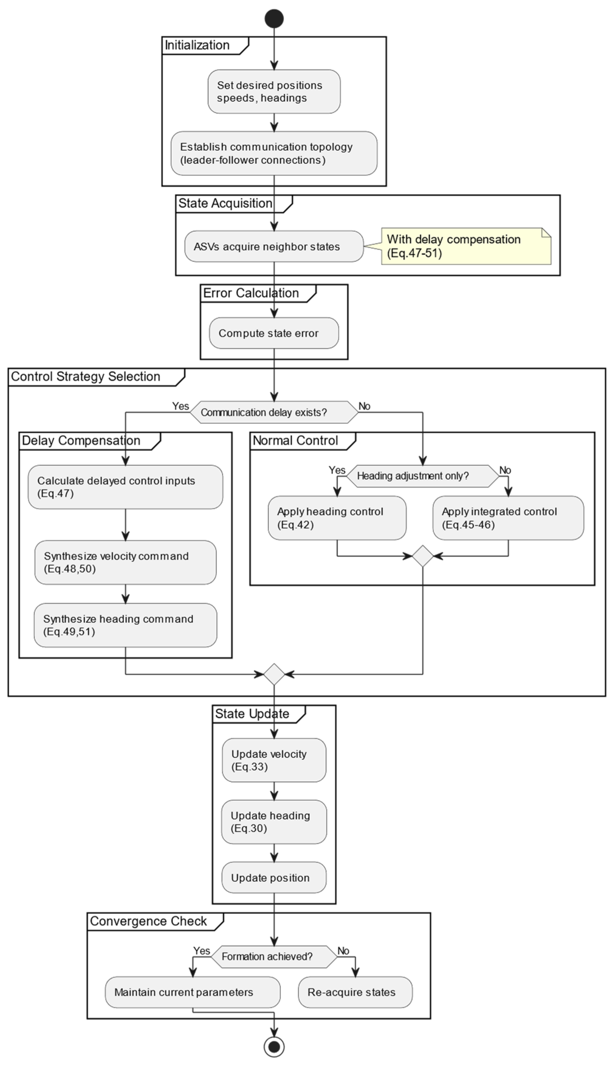
4.1. Cooperative Formation Control Strategy

Before designing cooperative formation control strategies, the stability of consensus under the communication topology is analyzed, and a fundamental consensus-based cooperative control strategy is presented.

4.1.1. Stability Analysis of Consensus Control Strategy

The formation of an ASV group is influenced by the communication topology within the formation. Therefore, it is essential to analyze the stability of the designed control strategies. For the formation communication topology, Ren proposed the consensus conditions for Lagrangian dynamics under a fixed communication topology.

Lemma 1. 

For entities with autonomous decision-making and execution capabilities, their state information equations can be represented using a double-integrator dynamic system, also known as a second-order system. The equations are as follows:

$${\dot{p}}_{\mathrm{i}}=q_{\mathrm{i}}, {\dot{q}}_{\mathrm{i}}=u_i$$

(13)

where  $p_i$  represents the state information of the i-th ASV,  $q_i$  corresponds to the derivative of the state information, representing the velocity, and $u_i$ is the control input for the i-th ASV. For motion systems that can be expressed using Equation (13), a consensus algorithm can be applied during formation control. The consensus algorithm is given as:

$$u_i=-{\sum }_j^n a_{ij}\left[\left(p_i-p_j\right)+\alpha \left(q_i-q_j\right)\right]$$

(14)

where  $\alpha$  is a positive scalar, representing the gain coefficient for the derivative changes between two moving entities.

Further, when directly considering higher-order multi-intelligent systems, the state equations can be represented as:

$$\left\{\begin{array}{c}{\dot{x}}_i^{(0)}=x_i^{(1)}\\ ⋮\\ {\dot{x}}_i^{(l-1)}=u_i\end{array}\right.$$

(15)

where $x_i^l\in R^m$ represents the state variable of information, $x_i^l$ represents the l-th order derivative of x_i, $x_i^{(0)}$ is the original state variable, and u_i is the control input. For the aforementioned higher-order system, a consensus algorithm for higher-order systems can be designed based on the second-order consensus algorithm referenced in the literature. The algorithm is as follows:

$$u_i=-{\sum }_{j\in N_i} a_{ij}\left[{\sum }_{k=0}^{l-1} {\alpha }_k\left(x_i^{(k)}-x_j^k\right)\right]$$

(16)

where ${\alpha }_k\in N,{ \alpha }_k\ne 0$ represent the weights of the state variables, when $x_i^{(k)}\to x_j^k$ indicates that the k-th derivatives of the state variables of agents i and j approach each other as time progresses. The multi-agent system achieves asymptotic stability when the states across agents converge.

Properly setting the state variable weights, α_k, is a critical step in designing the consensus algorithm. To address this, the following theorem is provided.

Lemma 2. 

In a multi-agent system with a minimum spanning tree, if the weights of the state variables α_k ensure that the system is Hurwitz-stable, the information of all agents can achieve consensus stability.

To prove this, control Algorithm (16) is substituted into the system Equation (17). This yields:

$$\left\{\begin{array}{c}{\dot{x}}_i^{(0)}=x_i^{(1)}\\ {\dot{x}}_i^{(1)}=x_i^{(2)}\\ ⋮\\ {\dot{x}}_i^{(l-1)}=-\sum _{j\in N_i} a_{ij}\left[\sum _{k=0}^{l-1} {\alpha }_k\left(x_i^{(k)}-x_j^k\right)\right]\end{array}\right.$$

(17)

where $x_i={\left[x_i^{(0)},x_i^{(1)},\cdots ,x_i^{(l-1)}\right]}^T$. To represent the system in state-space form, let $y_i=x_i$. The state-space matrix equation for the multi-agent system can be expressed as follows:

$$\left\{\begin{array}{c}{\dot{x}}_i=A^{\prime }{x}_i+B^l{u}_i\\ y_i=C^{\prime }{x}_i+D^{\prime }{u}_i\end{array}\right.$$

(18)

If $u_i$ is represented in matrix form, it can be expressed as follows:

$$u_i=\left[\begin{array}{c}-\sum _{j=1}^n l_{11}\left(x_i^{(0)}-x_j^{(0)}\right)\\ -\sum _{j=1}^n l_{22}\left(x_i^{(1)}-x_j^{(1)}\right)\\ ⋮\\ -\sum _{j=1}^n l_{ll}\left(x_i^{(l-1)}-x_j^{(l-1)}\right)\end{array}\right]$$

(19)

In this case, $l_{11},l_{22},\cdots ,l_n$, refer to the diagonal elements of the Laplacian matrix L, which are defined based on the communication topology. According to the definition of the Laplacian matrix:

$$A^{\prime }={\left[\begin{array}{ccccc}0& 1& 0& \cdots & 0\\ 0& 0& 1& \cdots & 0\\ ⋮& ⋮& ⋮& \ddots & ⋮\\ 0& 0& 0& \cdots & 1\\ 0& 0& 0& \cdots & 0\end{array}\right]}_{l\times l}, B^l={\left[\begin{array}{ccccc}0& 0& 0& \cdots & 0\\ 0& 0& 0& \cdots & 0\\ ⋮& ⋮& ⋮& \ddots & ⋮\\ 0& 0& 0& \cdots & 0\\ {\alpha }_0& {\alpha }_1& {\alpha }_2& \cdots & {\alpha }_{l-1}\end{array}\right]}_{l\times l}$$

(20)

For a high-order system, with $C^l$ as the l-order identity matrix and $D^l$ as the zero matrix, the stability analysis of the closed-loop system can be conducted. According to modern control theory, the open-loop transfer function of the system can be derived as follows:

$$G^l(s)=C^l\left(sI-A^l\right)B^l$$

(21)

After simplification, the matrix form of the open-loop transfer function for the high-order system can be expressed as:

$$G^l(s)=\left[\begin{array}{cccc}{\displaystyle \frac{{\alpha }_0}{s^l}}& {\displaystyle \frac{{\alpha }_1}{s^l}}& \dots & {\displaystyle \frac{{\alpha }_{l-1}}{s^l}}\\ {\displaystyle \frac{{\alpha }_0}{s^{l-1}}}& {\displaystyle \frac{{\alpha }_1}{s^{l-1}}}& \dots & {\displaystyle \frac{{\alpha }_{l-1}}{s^{l-1}}}\\ ⋮& ⋮& \ddots & ⋮\\ {\displaystyle \frac{{\alpha }_0}{s}}& {\displaystyle \frac{{\alpha }_1}{s}}& \dots & {\displaystyle \frac{{\alpha }_{l-1}}{s}}\end{array}\right]$$

(22)

The closed-loop transfer function matrix ${\varphi }^L(s)$ for the system satisfies the following form:

$${\varphi }^L(s)=G^l(s){\left(I_l+G^l(s)\right)}^{-1}$$

(23)

The characteristic polynomial of the closed-loop transfer function, which determines the eigenvalues of the system, satisfies the following relationship:

$$\mathrm{d}\mathrm{e}\mathrm{t}\left({\varphi }^l\left(s\right)\right)=\mathrm{d}\mathrm{e}\mathrm{t}\left(I_l+G^l\left(s\right)\right)\cdot \mathrm{d}\mathrm{e}\mathrm{t}\left(s{I}_l-A^l\right)$$

(24)

To compute the characteristic polynomial for the closed-loop system, we derive the determinants $\mathrm{d}\mathrm{e}\mathrm{t}\left(I_l+G^l(s)\right)$ and $\mathrm{d}\mathrm{e}\mathrm{t}\left(s{I}_l-A^l\right)$ as follows:

$$I_l+G^l(s)={\left[\begin{array}{cccc}1+{\displaystyle \frac{{\alpha }_0}{s^l}}& {\displaystyle \frac{{\alpha }_1}{s^l}}& \cdots & {\displaystyle \frac{{\alpha }_{l-1}}{s^l}}\\ {\displaystyle \frac{{\alpha }_0}{s^{l-1}}}& 1+{\displaystyle \frac{{\alpha }_1}{s^{l-1}}}& \cdots & {\displaystyle \frac{{\alpha }_{l-1}}{s^{l-1}}}\\ ⋮& ⋮& \ddots & ⋮\\ {\displaystyle \frac{{\alpha }_0}{s}}& {\displaystyle \frac{{\alpha }_1}{s}}& \cdots & 1+{\displaystyle \frac{{\alpha }_{l-1}}{s}}\end{array}\right]}_{l\times l}$$

(25)

By performing elementary row and column operations on Equation (25), we obtain:

$$I_l+G^l(s)={\left[\begin{array}{ccccc}1+{\displaystyle \frac{{\alpha }_0}{s^l}}+\cdots +{\displaystyle \frac{{\alpha }_{l-1}}{s}}& {\displaystyle \frac{{\alpha }_1}{s^l}}& {\displaystyle \frac{{\alpha }_2}{s^l}}& \cdots & {\displaystyle \frac{{\alpha }_{l-1}}{s^l}}\\ -s& 1& 0& \cdots & 0\\ 0& -s& 1& \cdots & 0\\ ⋮& ⋮& ⋮& \ddots & ⋮\\ 0& 0& \cdots & -s& 1\end{array}\right]}_{l\times l}$$

(26)

Expanding along the first column yields:

$$\mathrm{d}\mathrm{e}\mathrm{t}\left(I_l+G^l(s)\right)=1+{\displaystyle \frac{{\alpha }_0}{s^l}}+{\displaystyle \frac{{\alpha }_1}{s^{l-1}}}\cdots +{\displaystyle \frac{{\alpha }_{l-1}}{s}}$$

(27)

$$\mathrm{d}\mathrm{e}\mathrm{t}\left(s{I}_l-A^{\prime }\right)={\left[\begin{array}{ccccc}s& -1& 0& \cdots & 0\\ 0& s& -1& \cdots & 0\\ ⋮& & \ddots & & ⋮\\ 0& 0& \cdots & s& -1\\ 0& 0& \cdots & 0& s\end{array}\right]}_{\left|x\right|}=s^l$$

(28)

The closed-loop characteristic polynomial is expressed as:

$$\begin{array}{cc}\det \left({\varphi }^{\prime }(s)\right)& =\det \left(I_l+G^l(s)\right)\cdot det\left(s{I}_l-A^{\prime }\right)\\ & =\left(1+{\displaystyle \frac{{\alpha }_0}{s^l}}+{\displaystyle \frac{{\alpha }_1}{s^{l-1}}}\cdots +{\displaystyle \frac{{\alpha }_{l-1}}{s}}\right)\cdot s^l\end{array}$$

(29)

According to the polynomial stability theorem, the necessary and sufficient condition for the asymptotic stability of the closed-loop system is that all closed-loop poles (roots of the polynomial) lie in the left-half plane of the complex domain. Based on the Routh–Hurwitz criterion, the system is stable if ${\alpha }_0,{\alpha }_1,\cdots ,{\alpha }_{I-1}$ form a Hurwitz polynomial. If ${\alpha }_0,{\alpha }_1,\cdots ,{\alpha }_{I-1}$ satisfy the Hurwitz condition, the control strategy introduced in this section ensures that the state information of all system orders achieves consensus stability.

The subsequent cooperative formation control strategy and encirclement control strategy for unmanned surface vehicles, as discussed in later sections of this paper, are designed based on the principles in Equation (16).

4.1.2. State Control for Cooperative Motion

In the study of cooperative motion for multiple autonomous surface vehicles, state control is a critical factor that cannot be overlooked. The designed cooperative control strategy must ensure the convergence of state information for the ships to have practical significance. As discussed in the mathematical modeling section in Section 2, the heading angle and velocity are the two most important state variables, as they directly affect the motion trajectory of ships. Therefore, this study prioritizes the control of these two state variables.

Heading control is crucial for the state control of ships. The designed formation control strategy must ensure that the heading angles of all individual ships converge to a common value when the formation stabilizes. The simplified formula for the change in heading angle is expressed as:

$${\dot{\psi }}_i={\displaystyle \frac{1}{{\tau }_{\psi }}}\left({\psi }_i^c-{\psi }_i\right)$$

(30)

where ψ_i is the current heading angle of ASV i, ${\psi }_i^c$ is the desired heading angle generated by the formation control strategy, and ${\tau }_{\psi }$ is the time constant for heading adjustment.

The next stage heading angle of an ASV is calculated based on its current heading angle ${\psi }_i$ and the control command ${\psi }_i^c$. The control command ${\psi }_i^c$ is generated by the formation control strategy and integrates the heading angles of all ships in the formation at the same time, producing a control adjustment specific to ASV i.

As illustrated in Figure 4, consider three ships with initial heading angles ${\psi }_1>{\psi }_2>{\psi }_3$ through internal communication within the formation and adjustment based on the neighboring ships’ heading angles; the heading angles are gradually aligned, ultimately achieving ${\psi }_1={\psi }_2={\psi }_3$. During the adjustment process, the following constraint must be satisfied: $\left|\Delta {\psi }_i\right|<\pi$.

This ensures smooth convergence and avoids abrupt or excessive heading changes, facilitating stable and cooperative formation behavior. The consensus control strategy for the heading angle is given by:

$$\left\{\begin{array}{c}{\psi }_i^c={\psi }_i+{\displaystyle \frac{1}{1+n_i}}{u}_i\\ u_i=-\sum _{j=1}^n a_{ij}\left({\psi }_i-{\psi }_j\right)\end{array}\right.$$

(31)

where $n_i$ is the number of ships connected to ASV i in the communication topology, $a_{ij}$ is the weight of the adjacency matrix in the communication topology, and $u_i$ is the cooperative control term for the heading angle of ASV i. Traditional methods use Equation (31) for heading control. However, this approach cannot guarantee that the ships reach the desired heading angle, meaning it cannot determine the final attitude. This paper proposes an improved control strategy based on consensus theory to ensure convergence of the ships’ heading angles. The improved method is as follows:

$$\left\{\begin{array}{c}{\psi }_i^c={\psi }_i+{\displaystyle \frac{1}{1+n_i}}{u}_i\\ u_i=-b_i\left({\psi }_i-{\psi }^q\right)-\sum _{j=1}^n a_{ij}\left({\psi }_i-{\psi }_j\right)\end{array}\right.$$

(32)

where $u_i$ is the cooperative control term, composed of two parts, and $b_i$ is the coefficient of the desired tracking term. The velocity variation formula for the formation can be simplified as:

$${\dot{v}}_i={\displaystyle \frac{1}{{\tau }_v}}\left(v_i^c-v_i\right)$$

(33)

The consistency control strategy for speed convergence to the expected value is as follows:

$$\left\{\begin{array}{c}{v}_i^c=v_i+{\displaystyle \frac{1}{1+n_i}}{u}_i\\ u_i=-c_i\left(v_i-v^q\right)-\sum _{j=1}^n a_{ij}\left(v_i-v_j\right)\end{array}\right.$$

(34)

Then, the characteristic model-based intelligent adaptive control of $\psi$ and $\psi$ can be designed based on our research [1], with the controllers involved achieving tracking control of the desired ship state.

4.1.3. Cooperative Formation Control Strategy Based on Consensus Theory

In addition to ensuring that the heading angles and velocities of all ships converge, formation control must also ensure that the positions of all ships form a specific formation. Therefore, under the condition of a communication topology, a cooperative formation control strategy is designed based on consensus theory to enable ships to autonomously form a given formation. Since ships operate in a two-dimensional space, the design of the cooperative formation control strategy only needs to consider the North and East directions.

When the ships have not completed the formation task, the desired spacing between vehicles in the final formation must be obtained from the communication topology structure. For ASV i, the completion of the formation task must satisfy the following conditions, as shown in Equation (35):

$$\begin{array}{c}\left(x_i^{\prime }-x_{iF}^{\prime }\right)-\left(x_j^{\prime }-x_{jF}^{\prime }\right)=0\\ \left(y_i^{\prime }-y_{iF}^{\prime }\right)-\left(y_j^{\prime }-y_{jF}^{\prime }\right)=0\end{array}$$

(35)

Simplifying these equations yields:

$$\begin{array}{c}{x}_i^{\prime }-x_j^{\prime }-x_{ij}^{\prime q}=0\\ y_i^{\prime }-y_j^{\prime }-y_{ij}^{\prime q}=0\end{array}$$

(36)

where $x_{ij}^{\prime q},y_{ij}^{\prime q}$ represent the desired spacing between ASV i and its neighboring ASV j in the communication topology.

Assume the current position of ASV i is p; to achieve the formation, ASV i adjusts its heading angle and velocity to reach position pi′. The velocity components in the X- and Y-axes are given as:

$$v_i^{\prime x}=v_i\cos \Delta {\psi }_i$$

(37)

$$v_i^{\prime y}=v_i\sin \Delta {\psi }_i$$

(38)

During the process of forming the predetermined formation, the heading angle and velocity—two critical state variables—are continuously changing. The cooperative formation control strategy based on consensus theory is expressed as:

$$v_i^c=v_i-{\sum }_{j=1}^n a_{ij}\left[{\tau }_{\mathrm{r}}\left(v_i-v_j\right)+k_i^{\mathrm{v}\mathrm{c}\mathrm{h}}\left(x_i^{\prime }-x_j^{\prime }-x_{ij}^{\prime q}\right)\right]$$

(39)

$${\psi }_i^c={\psi }_i-{\sum }_{j=1}^n a_{ij}\left[{\displaystyle \frac{1}{1+n_i}}\left({\psi }_i-{\psi }_j\right)+k_i^{\psi ch}\left(y_i^{\prime }-y_j^{\prime }-y_{ij}^{\prime q}\right)\right]$$

(40)

where $k_i^{\mathrm{v}ch},k_i^{\psi ch}$ represent the variable gains that measure the influence of the desired formation spacing on the control commands. Their values become 0 when the formation is achieved.

Using Equations (39) and (40), ships with different initial positions and states can form a specified formation, and their heading angles and velocities will converge to a consistent state. During the actual motion of ASV formations, specific motion directions and speeds are assigned based on different task requirements, and different control strategies are adopted accordingly. The following three improved algorithms are proposed:

$$v_i^c=v_i-{\sum }_{j=1}^n a_{ij}\left[{\tau }_v\left(v_i-v_j\right)+k_i^{vch}\left(x_i^{\prime }-x_j^{\prime }-x_{ij}^{\prime q}\right)\right]$$

(41)

$${\psi }_i^c={\psi }_i-b_i^{ch}\left({\psi }_i-{\psi }^q\right)-{\sum }_{j=1}^n a_{ij}\left[{\displaystyle \frac{1}{1+n_i}}\left({\psi }_i-{\psi }_j\right)+k_i^{\psi ch}\left(y_i^{\prime }-y_j^{\prime }-y_{ij}^{\prime q}\right)\right]$$

(42)

By using Equations (40)–(42), the direction of convergence of the formation can be made to reach ${\psi }^q$:

$$v_i^c=v_i-c_i^{ch}\left(v_i-v^q\right)-{\sum }_{j=1}^n a_{ij}\left[{\tau }_v\left(v_i-v_j\right)+k_i^{vch}\left(x_i^{\prime }-x_j^{\prime }-x_{ij}^{\prime q}\right)\right]$$

(43)

$${\psi }_i^c={\psi }_i-{\sum }_{j=1}^n a_{ij}\left[{\displaystyle \frac{1}{1+n_i}}\left({\psi }_i-{\psi }_j\right)+k_i^{\psi ch}\left(y_i^{\prime }-y_j^{\prime }-y_{ij}^{\prime q}\right)\right]$$

(44)

By using Equations (43) and (44), the convergence speed of the formation can be set to $v^q$:

$$v_i^c=v_i-c_i^{ch}\left(v_i-v^q\right)-{\sum }_{j=1}^n a_{ij}\left[{\tau }_v\left(v_i-v_j\right)+k_i^{vch}\left(x_i^{\prime }-x_j^{\prime }-x_{ij}^{\prime q}\right)\right]$$

(45)

$${\psi }_i^c={\psi }_i-b_i^{ch}\left({\psi }_i-{\psi }^q\right)-{\sum }_{j=1}^n a_{ij}\left[{\displaystyle \frac{1}{1+n_i}}\left({\psi }_i-{\psi }_j\right)+k_i^{\psi ch}\left(y_i^{\prime }-y_j^{\prime }-y_{ij}^{\prime q}\right)\right]$$

(46)

By constructing a reasonable communication topology within the ASV group and combining the algorithms described in Equations (43) and (44) through (45) and (46), the ASV cluster can effectively achieve the desired formation in a two-dimensional plane. These algorithms ensure that the heading angle, velocity, and relative positions between ships converge to the specified formation parameters, enabling efficient and robust cooperative formation control.

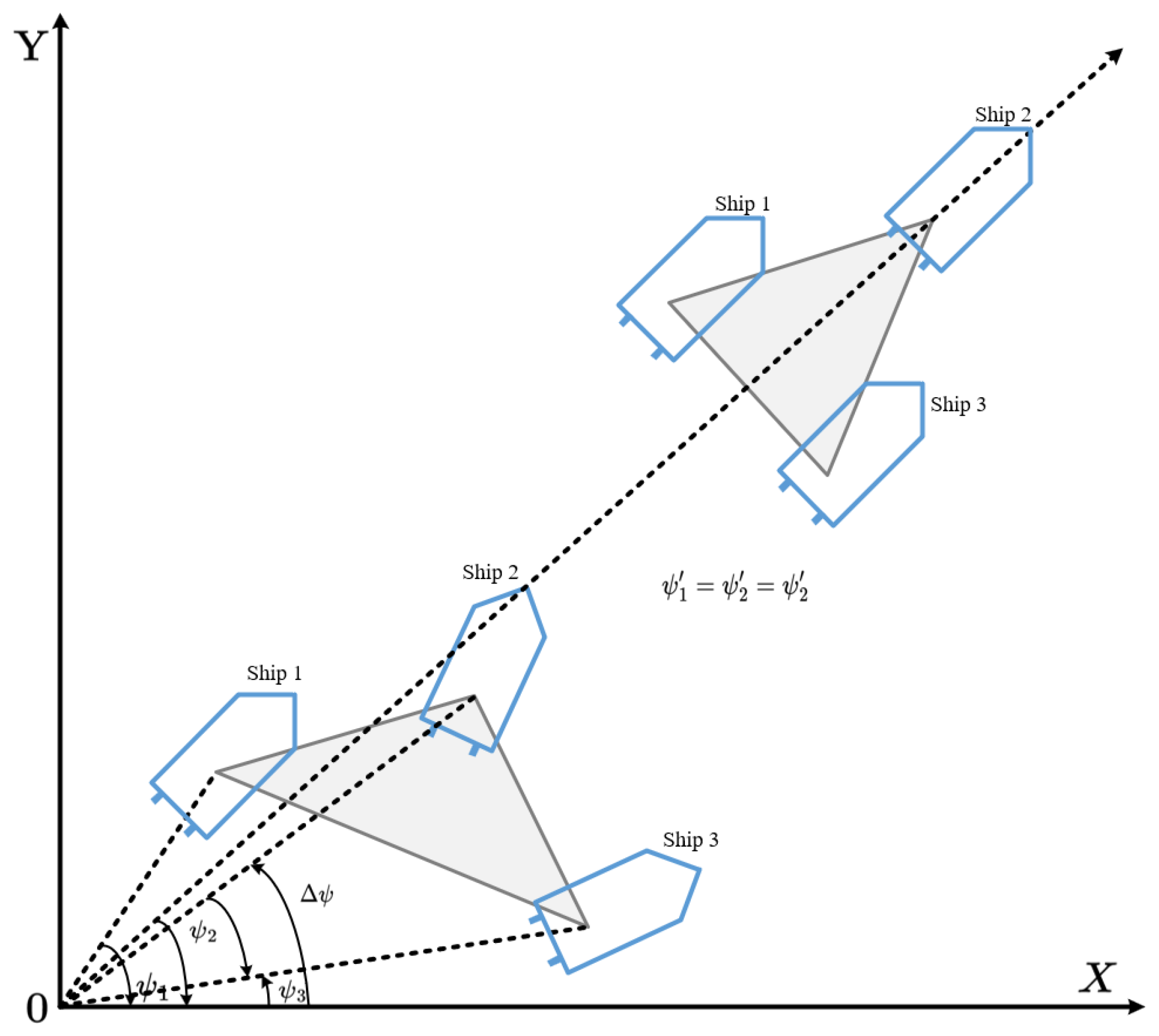
4.1.4. Formation Maintenance and Transformation of ASV Formations

During the execution of tasks by an ASV formation, the formation system may adapt to different tasks by adjusting its heading angles and velocities. Sometimes, only one state variable is adjusted, while at other times, both heading angles and velocities are changed simultaneously. Therefore, it is essential to ensure that the ASV formation can perform autonomous cooperative motion under any circumstance.

The previous section identified that factors influencing computational burden include the complexity of the algorithm and the number of variables. Considering that during ASV formation movement, there are scenarios where only one state variable (heading angle or velocity) needs to change, while in others, both must change simultaneously, different formation control strategies should be adopted accordingly. The following introduces two cases.

During the task execution process, when the task point’s position changes or an obstacle appears in the path ahead, the formation control strategy described in Equations (41) and (42) can be used to reset the heading angle of the ASV formation.

When performing target tracking tasks, where the target’s position and state continuously change, the ASV formation needs to utilize the formation control strategy described in Equations (45) and (46). This enables the ships to adjust their heading angles and velocities in real-time based on the target’s position and state information. By employing the strategies provided above, ASV formations can effectively complete various tasks. Part of these formation control strategies will be validated in the simulation section.

4.2. Cooperative Control Strategies for Formations Under Delay

During the motion of an ASV formation, individual ships must exchange information with others to understand their motion states. However, in practical formation experiments, issues such as communication delay, noise, and packet loss are unavoidable. Therefore, delays must be considered in the design and implementation of formation control strategies.

4.2.1. Sources of Communication Delays

Communication delay is the time required for a signal to travel from one agent to another. It depends on the communication medium and the physical distance between the agents. Longer distances or slower communication mediums result in longer transmission times. The communication diagram and controller diagram of an unmanned ship are shown in Figure 5.

Communication delays can severely impact the performance of formation control algorithms. The key challenges caused by delays include lag in feedback and instability in the formation. When agents rely on outdated information from neighbors, it can result in decisions based on inaccurate positions or velocities, leading to inefficient coordination and delayed responses in formation adjustments. In some cases, long delays can prevent the system from achieving consensus, causing the formation to oscillate or fail to reach a stable state.

The stability of the delay-based consensus formation cooperative control strategy was demonstrated in the previous section. Therefore, it is crucial to study the communication topology structure of ASV formations under delay conditions. The delay communication topology structure increases the number of undirected paths between nodes, reducing the dependence on single sources of information. The structure is shown in Figure 6.

The internal communication topology of ships plays a crucial role in ensuring formation control. Forming a directed spanning tree is a necessary condition for achieving convergence and consensus in the formation. The main advantage of the delay communication model is that while building upon the strong connectivity structure, it increases the feedback among ships, thereby reducing communication delays during the formation process.

Additionally, this topology provides some level of protection for individual ships. For example, if there are differences in the construction costs of various ships, the communication topology architecture can leverage these differences through weight coefficients to influence the formation. Higher-cost ships, often with better communication capabilities, act as primary nodes, and other ships adjust their formation direction relative to these primary nodes.

For addressing the delay issue in ASV formations, adopting the delay communication model offers significant advantages. It ensures formation convergence, enhances feedback, and optimizes the communication structure by prioritizing critical nodes. This approach reduces the maximum directed path threshold, making the formation more robust and efficient.

4.2.2. Control Strategies for Delayed Formations Based on Consensus Theory

Communication delays within an ASV formation mean that the state of an ASV at the next time step is influenced not only by its current state but also by the previous states of other ships. Thus, the control strategy for delayed formations must account for providing control inputs to the ships. Ensuring the stability of the cooperative control strategy under delay conditions. To address the negative effects of communication delays, we developed a consensus mechanism within the control algorithm.

By considering the synchronous coupling method, it is possible to achieve state synchronization among the formation ships. This method is applied to the cooperative control strategy by using the delayed state of the previous time step to construct the control input for the current time step.

The control components for the ASV formation in the X- and Y-plane dimensions are given as:

$$\left\{\begin{array}{c}{u}_i^x=-{\eta }_1{\sum }_{j\in N_i} \left[x_i(t-\tau )-x_j(t-\tau )-d_{ij}^x\right]-{\eta }_2{\sum }_{j\in N_i} \left[v_i^x(t)-v_j^x(t)\right]+{\eta }_2{b}_i\left[v_o(t)-v_i^x(t)\right]\\ u_i^y=-{\eta }_1{\sum }_{j\in N_i} \left[y_i(t-\tau )-y_j(t-\tau )-d_{ij}^y\right]-{\eta }_2{\sum }_{j\in N_i} \left[v_i^y(t)-v_j^y(t)\right]+{\eta }_2{b}_i\left[v_o(t)-v_i^y(t)\right]\end{array}\right.$$

(47)

To combine the control components in the X- and Y-directions, the velocity and heading angle control commands for formation ships are derived based on the ASV kinematic model:

$$v_i^c=v_i+{\tau }_v\left(u_i^x\cos {\psi }_i+u_i^y\sin {\psi }_i\right)$$

(48)

$${\psi }_i^c={\psi }_i+{\displaystyle \frac{{\tau }_{\psi }}{v}}\left(u_i^y\cos {\psi }_i-u_i^x\sin {\psi }_i\right)$$

(49)

Further, the precise control commands with added desired convergence values are given as:

$$v_i^c=v_i-c_i\left(v_i-v^q\right)+{\tau }_v\left(u_i^x\cos {\psi }_i+u_i^y\sin {\psi }_i\right)$$

(50)

$${\psi }_i^c={\psi }_i-b_i\left({\psi }_i-{\psi }^q\right)+{\displaystyle \frac{{\tau }_{\psi }}{v}}\left(u_i^y\cos {\psi }_i-u_i^x\sin {\psi }_i\right)$$

(51)

The above strategy enables the effective cooperative control of multi-ASV formations under delayed conditions. By combining kinematic modeling with precise control adjustments for the velocity and heading angle, the strategy ensures the formation can achieve the desired configuration while compensating for communication delays.

The following block diagrams shown in Figure 7 illustrate the steps involved in the proposed consensus-based formation control strategy. The diagrams show the flow of information through the system, from the initial measurement of the relative positions, velocities, and headings of the ASVs to the computation of control inputs. The diagrams also demonstrate how the communication topology and time delays are incorporated into the control process to adjust the control inputs accordingly.

4.2.3. Stability Proof of Cooperative Control Strategies Under Delay

In this subsection, we prove the stability of the cooperative control strategy under delay conditions for ASV formations, as designed in the previous section. Assume the state information of ASV i is represented by $p_i={\left[x_i,y_i\right]}^T,q_i={\left[v_i^x,v_i^y\right]}^T$ For the ASV formation construct $p={\left[p_1,p_2,\cdots p_n\right]}^T$, the formation system is modeled using a double-integrator dynamic system based on the motion characteristics of ASV formations. By substituting the control inputs derived from the delayed formation control strategy into the system equations, we obtain:

$$\left\{\begin{array}{c}\dot{p}(t)=q(t)\\ \dot{q}(t)=-{\eta }_1\left[Lp(t-\tau )-\mathrm{d}\mathrm{i}\mathrm{a}\mathrm{g}\left(A{R}_1\right)\right]-{\eta }_2(L+B)\left[q(t)-v_o(t)\otimes I_n\right]\end{array}\right.$$

(52)

where A is the adjacency matrix, $R_1=\left[{\mathrm{r}}_{ij}\right]$ is the desired formation spacing matrix $r_{ij}={\left[r_{ij}^x,r_{ij}^y\right]}^T$ represents the desired spacing in the x- and y-directions, and $I_n=[1,\cdots ,1{]}^T$ is identity vector.

Let $Lp(t-\tau )-\mathrm{d}\mathrm{i}\mathrm{a}\mathrm{g}\left(A{R}_1\right)=\overline{p}(t),q(t)-v_o(t)\otimes I_n=\overline{q}(t)$; the system then transforms to:

$$\left\{\begin{array}{c}\dot{\overline{p}}(t)=l\overline{q}(t)\\ \dot{q}(t)=-{\eta }_1\overline{p}(t-\tau )-{\eta }_2(L+B)\overline{q}(t)\end{array}\right.$$

(53)

Further, define $[\overline{p}(t),\overline{q}(t)]=w(t)$, and the system becomes:

$$\dot{w}(t)=\left[\begin{array}{cc}0& L\\ 0& -{\eta }_2(B+L)\end{array}\right]w(t)+\left[\begin{array}{cc}0& 0\\ -{\eta }_1{I}_n& 0\end{array}\right]w(t-\tau )$$

(54)

To analyze stability, we construct a Lyapunov–Krasovskii function as follows:

$$V(t)=w^T(t)Pw(t)+{\int }_{t-\tau }^t w(s)Qw(s)ds+{\int }_{-f}^0 {\int }_{t+\theta }^t {\dot{w}}^T(s)R\dot{w}(s)d\theta ds$$

(55)

Taking the derivative of $V(t)$ gives:

$$\begin{array}{c}\dot{V}(t)=2w^T(t)P\dot{w}(t)+w^T(t)Qw(t)-w^T(t-\tau )Qw(t-\tau )\\ +\tau {\dot{w}}^T(t)R\dot{w}(t)-{\int }_{t-\tau }^t {\dot{w}}^T(s)R\dot{w}(s)ds\end{array}$$

(56)

Then, we obtain:

$$\dot{w}(t)=Ew(t)+Fw(t-\tau )$$

(57)

We can obtain the following:

$$2w^T(t)P\dot{w}(t)=2w^T(t)P(Ew(t)+Fw(t-\tau ))$$

(58)

For any $x,y\in R^n$ and positive definite matrix $M\in R^{n\times n}$, the following can be obtained:

$$2x^{T}y\le x^T{M}^{-1}x+y^{T}My$$

(59)

For Equation (59), there are:

$$\begin{array}{cc}2w^T(t)PFw(t-\tau )& =2w^T(t)PF\left[w(t)-{\int }_{t-\tau }^t \dot{w}(s)ds\right]\\ & =2w^T(t)PFw(t)-2w^T(t)PF{\int }_{t-\tau }^t \dot{w}(s)ds\\ & \le 2w^T(t)PFw(t)+\tau w^T(t)PF{R}^{-1}{F}^{T}Pw(T)+{\int }_{t-\mathrm{r}}^t {\dot{w}}^T(s)R\dot{w}(s)ds\end{array}$$

(60)

Furthermore, for the integral terms within Equation (61), there are:

$$\begin{array}{l}{\int }_{1-t}^t {\dot{w}}^T(s)R\dot{w}(s)ds=\tau [Ew(t)+Fw(t-\tau ){]}^{T}R[Ew(t)+Fw\left(t-\tau \right)]\\ =\tau w^T(t)E^{\tau }REw(t)+\tau w^T(t-\tau )F^{\tau }REw(t)+\\ \tau w^T(t)E^{T}RFw(t-\tau )+\tau w^T(t-\tau )F^{T}REw(t-\tau )\end{array}$$

(61)

Furthermore, Equation (57) can be converted into:

$$\begin{array}{l}\dot{V}(t)\le 2w^T(t)PFw(t)+\tau w^T(t)PF{R}^{-1}{F}^{T}Pw(t)+w^T(t)Qw(t)\\ -w^T(t-\tau )Qw(t-\tau )+\tau w^T(t)E^{T}REw(t)+\tau w^T(t-\tau )F^{T}REw(t)\\ +\tau w^T(t)E^{T}RFw(t-\tau )+\tau w(t-\tau )F^{T}REw(t-\tau )\end{array}$$

(62)

Further, extracting the variables from Equation (63) gives:

$$N=(E+F{)}^{T}P+P(E+F)+\tau E^{T}RE+\tau PF{R}^{-1}{F}^{T}P+Q$$

(63)

where

$$\begin{array}{ll}\dot{V}(t)& \le {\left[\begin{array}{c}w(t)\\ w(t-\tau )\end{array}\right]}^T\left[\begin{array}{cc}N& \tau E^{T}RF\\ & \tau F^{T}RF-Q\end{array}\right]\left[\begin{array}{c}w(t)\\ w(t-\tau )\end{array}\right]\\ & \le {\left[\begin{array}{c}w(t)\\ w(t-\tau )\end{array}\right]}^{T}M\left[\begin{array}{c}w(t)\\ w(t-\tau )\end{array}\right]\end{array}$$

(64)

According to the Schur complement lemma, for a given symmetric matrix $X\in R^{n\times n}$, it can be partitioned as follows:

$$X=\left[\begin{array}{c}{x}_{11}\hspace{0.25em}\hspace{0.25em}\hspace{0.25em}\hspace{0.25em}{x}_{12}\\ x_{21}\hspace{0.25em}\hspace{0.25em}\hspace{0.25em}\hspace{0.25em}{x}_{22}\end{array}\right]$$

(65)

where $x_{11}\in R^{m\times m}, x_{22}\in R^{(n-m)\times (n-m)}, x_{12}=x_{21}^T, x_{21}\in R^{(n-m)\times m}, x_{12}\in R^{m\times (n-m)}$.

Then, X < 0 if and only if either of the following conditions are satisfied: $x_{11}<0,x_{22}-x_{21}{x}_{11}^{-1}{x}_{12}<0$ or $x_{22}<0,x_{11}-x_{12}{x}_{22}^{-1}{x}_{21}<0$.

Define $N_1=(E+F{)}^{T}P+P(E+F)+\tau E^{T}RE+Q$. For the matrix M in Equation (65), we have:

$$M=\left[\begin{array}{ccc}{N}_1& PF& \tau E^{\tau }RF\\ \ast & -{\displaystyle \frac{R}{\tau }}& 0\\ \ast & \ast & \tau F^{\tau }RF-Q\end{array}\right]$$

(66)

Using the Schur complement lemma, $M$ < 0 can be determined by ensuring the conditions of the lemma are satisfied. Once $M<0$ is confirmed, Equation (66) yields $\dot{V}(t)<0$.

Based on the Lyapunov stability theorem, $\dot{V}(t)<0$ ensures that the formation control strategy under delay conditions stabilizes the formation. This means that applying the proposed delay-based cooperative control strategy enables the ASV formation to maintain stability and achieve the desired formation even under communication delay conditions. Thus, for formations with a directed spanning tree communication topology and positive definite symmetric matrices satisfying Equation (66), the consensus-based formation control strategy designed in this study ensures that the ASV cluster can complete formation tasks in the presence of communication delays.

5. Simulation Verification of Multi-ASV Cooperative Formation Control Strategy

This section validates the designed cooperative formation control strategy through simulations. In this study, three experiments were conducted to design and validate the consistency-theory-based formation control under the delay of the formation.

5.1. Parameter Selection

The model we used in the simulation experiments was obtained by parameter identification based on a real twin-propulsion ship and real experimental data. Figure 8 shows the real twin-propulsion ASV used in our simulation. This ASV was predeveloped by us (as described in [44]) and a simulation model based on the feature model was built for it. This ASV is equipped with two 24 V thrust motors with a maximum thrust of 55 N. The length, width, and distance of the vessel from the propulsion motors are about 1.7, 0.75, and 0.5 m, respectively.

Based on the above unmanned ship model, three sets of experiments were carried out in this thesis to verify the effectiveness of the formation cooperative control algorithm based on the consistency theory, the cooperative control strategy under the formation time delay, and the comparison of the cooperative control under different control parameters, respectively. For the experiments conducted in this study, the simulation was performed using MATLAB 2023 a for modeling the system dynamics, control algorithm development, and simulation of the formation control strategy. MATLAB 2023 a provided a robust platform for implementing the control laws and performing the necessary computations. Additionally, to simulate real-time communication between the ASVs, we utilized the Robot Operating System 1(ROS 1). ROS 1 facilitated the integration of various system components, including communication between the ASVs and the simulation environment. It also allowed for the simulation of sensor data exchange and actuator control in real time, ensuring a more realistic representation of the cooperative behavior and interactions between the ASVs.

In Case I, the cooperative formation control algorithm based on consensus theory, as designed in the previous section, was applied. The parameter values in the control algorithm were set as $k_i^{wh}=k_i^{zch}=1.1/t, k_i^{ych}=\sqrt{{\displaystyle \frac{1.1}{t}}}, \eta =1.2$. The formation was set to achieve a square formation, with the velocity maintained at 1.5 m/s and the heading angle changing dynamically to enable circular motion. The corresponding formation matrix is as follows:

$$K^x=\left[\begin{array}{cccc}0& 75& 0& 75\\ -75& 0& 0& -75\\ -75& 0& 0& -75\\ 0& 75& 75& 0\end{array}\right], K^y=\left[\begin{array}{cccc}0& 0& 59& 59\\ 0& 0& 59& 59\\ -59& -59& 0& 0\\ -59& -59& 0& 0\end{array}\right]$$

To demonstrate the excellence of designed method for formation control, other algorithms were used to compare with the method in this paper. In the longitudinal direction, two good formation control methods [41,42,43] were selected.

In Case II, the algorithm coefficients were set as ${\eta }_1=0.73,{\eta }_2=1.02,b_i=0.8$. The desired formation was a diamond shape, with a desired heading angle of π/4. The initial position of ASV 1 was [36, −5], the horizontal velocity was 0.8, and the angle of direction was 0.59 rad. The initial position of ASV 2 was [20, 8], the horizontal velocity was 2.8, and the angle of direction was 0.38 rad. The initial position of ASV 3 was [7, −2], the horizontal velocity was 3.8, and the angle of direction was 1.22 rad. The initial position of ASV 4 was [23, −8], the horizontal velocity was 1.8, and the angle of direction was 0.89 rad. The transmission delay caused by data exchange was approximately 220 ms. Considering the high volume of data communication among the four ships, the simulation assumed a random communication delay ranging from 0.7 s to 1.2 s. The communication topology structure is shown in Figure 6. The cooperative control strategy based on consensus theory under delay conditions was applied to control the state variables of the ships within the formation.

In Case III, the experimental trajectory was parameterized as $x_R=t, y_R=20\cdot \mathrm{s}\mathrm{i}\mathrm{n}(0.05t)$. The control method and control parameters of the second group of experiments were adopted, and the control parameters were set as the first group, while the second group of control parameters was set, and the controller under the second group of control parameters was set as the control group to explore the effect of the change in the control parameters on the experimental results. The first set of parameters was set as ${\eta }_1=0.73, {\eta }_2=1.02, b_i=0.8$, and the second set of parameters was set as ${\eta }_1=0.93, {\eta }_2=1.42, b_i=0.8$. The initial position of the leader was [−45, −5, 0]. The initial position of the first follower was [−53, −13, 0], and the relative position of its formation was [−5, −5]. The initial position of the second follower was [−53, −2, 0], and the relative position of its formation was [−5, 5]. The desired speed in the experimental setup was 1.2 m/s. The main parameter settings are shown in

Table 2. Main parameter settings.

Parameter	Value
	Case 1	Case 2	Case 3
$\eta$	1	0.73, 1.02	1st 0.73, 1.02; 2nd 0.93, 1.42.
initial position of ASV 1	[19, 0]	[36, −5]	[−53, −13, 0]
initial position of ASV 2	[8, 0]	[20, 8]	[−5, −5]
initial position of ASV 3	[0, 0]	[7, −2]	[−53, −2, 0]
initial position of ASV 4	[32, 0]	[23, −8]	[−5, 5]

.

5.2. Results and Analysis

The results of our simulations and the analysis of these results are presented in this section. The simulations were designed to test the effectiveness of the cooperative formation control strategy, especially under conditions involving time delays. The experiments were conducted in three cases, each testing different aspects of the control strategy.

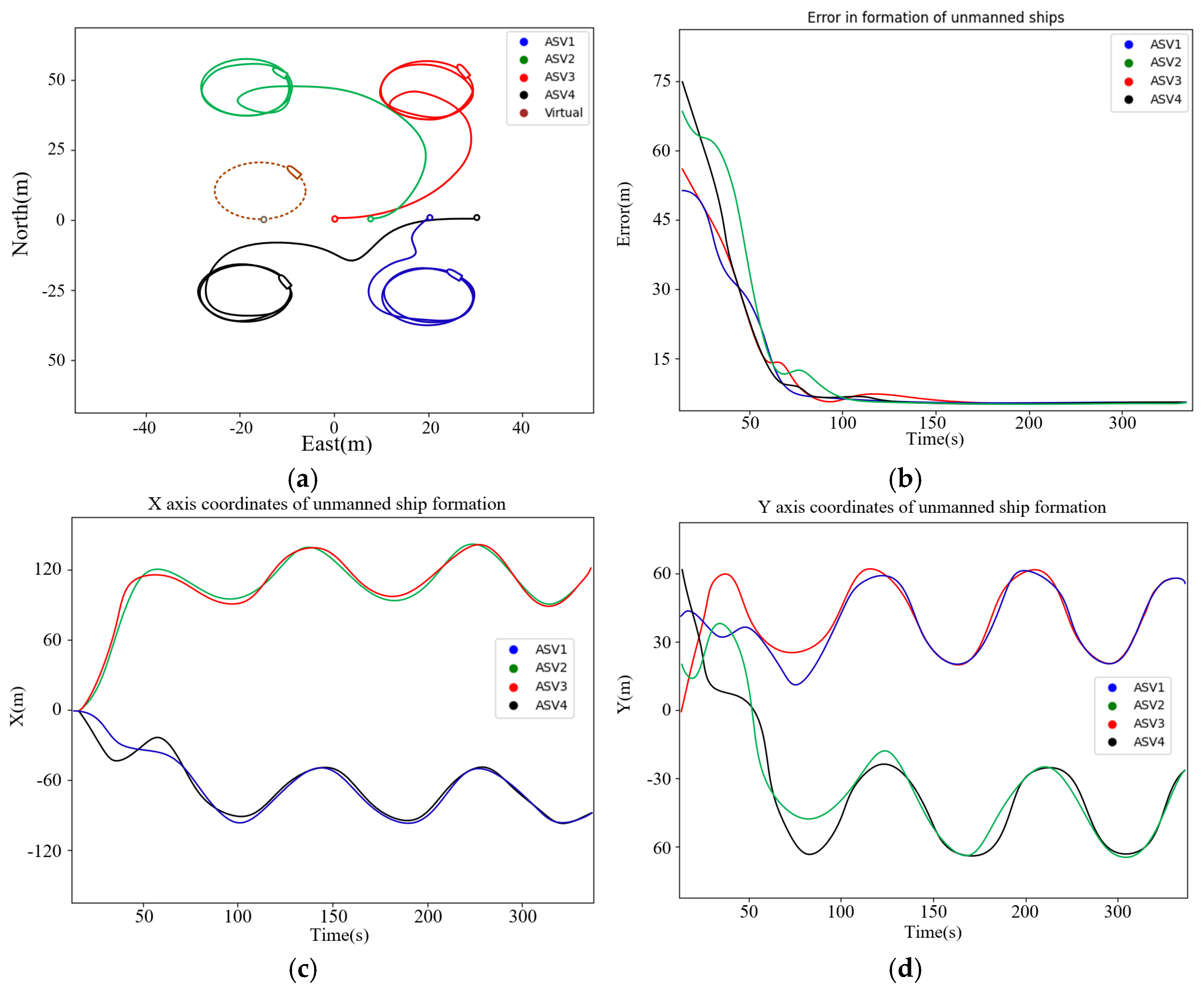
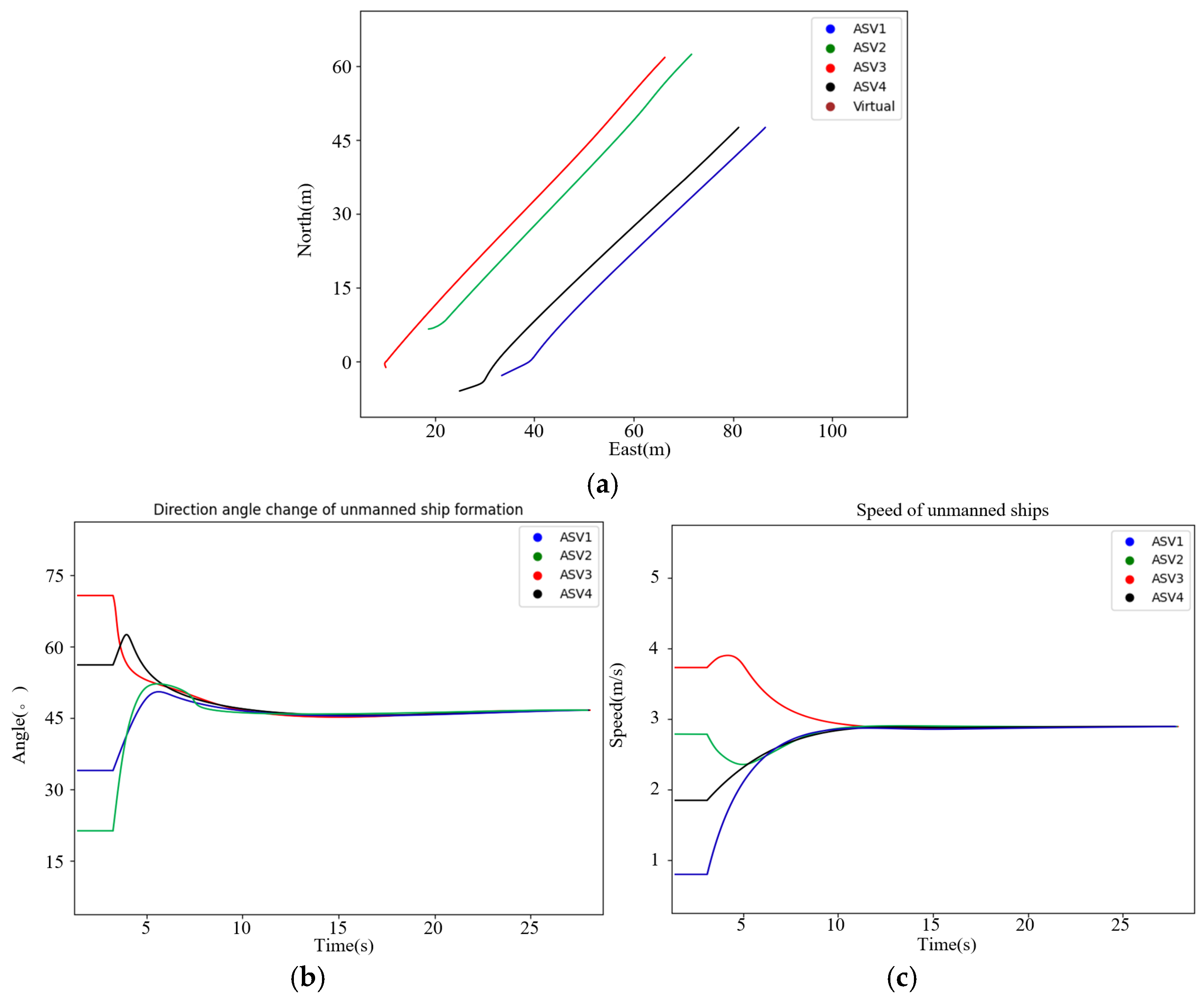
5.2.1. Case I: Circular Cooperative Formation Control

In this experiment, the ships were tasked with forming a square formation while maintaining circular motion. The formation was achieved successfully, as shown in the trajectory results (Figure 9). The results confirm that the proposed consensus-based cooperative formation control strategy effectively guided the ships to their target positions. The virtual ship in Figure 8 served as an idealized reference to evaluate the performance of the actual ASVs in the formation. It was not a physical entity but rather a computational model that represented the perfect trajectory and positioning of the ASVs in the formation, assuming no errors or delays. The inclusion of the virtual ship allowed for a clear comparison between the ideal and real behaviors of the ASVs, helping to highlight the deviations caused by factors such as communication delays, velocity constraints, and heading adjustments.

By comparing the actual ASVs with the virtual ship, we can assess how well the formation control algorithm performed and whether the ASVs maintained the desired formation under realistic conditions. For the formation trajectory, as shown in Figure 9a, the four ships, starting from different initial positions, utilized the proposed control strategy to eventually form a square formation while maintaining circular motion. Although the trajectories intersected in space, ships passed through the same points at different times, preventing collisions. The coordinate system used in Figure 9 is a standard Cartesian coordinate system (X, Y), which allows for a clear representation of the relative positions and movements of the ships. The “ground truth” was defined as the reference system from which these coordinates were derived, ensuring that all position data presented in the figure are based on a consistent frame of reference.

From Figure 9c,d, it can be observed that the final positions of ASV1 and ASV2 converged to the same state in the Y direction, while maintaining the given formation spacing in the X direction. Similarly, ASV2 and ASV4 converged to the same state in the X direction, while maintaining the given formation spacing in the Y direction. This demonstrates that, within a finite time, the four ships with different initial positions and states successfully formed a formation. In our study, the formation error stabilized at approximately 7 m after 100 s of operation. In contrast, previous methods, such as those proposed by [41,42,43], resulted in formation errors of 11 m, 10 m, and 13 m, respectively, under similar conditions. This shows that our approach achieved a more accurate formation with less deviation. Our method converged to the desired formation in about 100 s. Refs. [41,42] achieved convergence in 120 s, while [43] reported a convergence time of 150 s. The shorter convergence time of our approach suggests better efficiency in forming the desired configuration.

Table 3. Comparison of mean trajectory tracking errors for the heterogeneous MSV system.

Error	Proposed	DEFSMFC	NONNS	NOETC
ea(m)	7.605	10.895	10.0975	13.3825
eAsv1(m)	9.73	11.91	11.39	13.51
eAsv2 (m)	8.60	10.63	17.6	14.38
eAsv3 (m)	5.31	9.81	10.31	10.73
eAsv4 (m)	6.78	11.23	1.090	14.91

presents the results of the comparison of the average trajectory tracking error values between the control method used in this paper and the comparison method. As can be seen from the table, the method proposed in this paper had smaller tracking errors.

In conclusion, the consensus-based cooperative formation control strategy designed in the previous sections enables ships with different initial states and positions to effectively form a predetermined formation and achieve circular motion.

5.2.2. Case II: Cooperative Control Strategy Under Delays

This experiment was conducted to evaluate the control strategy under communication delays. The ships were tasked with forming a diamond-shaped formation.

The results of the formation trajectory, shown in Figure 10a, indicate that despite the delays, the ships successfully formed the diamond-shaped formation.

The responses of the heading angle and speed of each ship in the first thirty seconds are presented in Figure 10b,c. The results demonstrate that the delay-based cooperative control strategy enabled the ships to converge in both heading angle and speed. The system remained stable despite the communication delays.

A significant feature of this experiment is that the control strategy could adapt to delays, allowing the ships to achieve consensus in a reasonable time. The 220 ms delay was handled effectively, demonstrating the robustness of the control strategy under real-world conditions. In our simulations, the 220 ms delay was considered acceptable because our method adapted to this delay through the adaptive control strategy and ensured that the system remained stable. The results from our simulations, which show minimal formation errors and stable control under this delay, are provided to substantiate this claim. Our experiment was conducted under ideal conditions in an obstacle-free environment, and with a fixed 220 ms delay, the algorithm of our proposed new framework was effective. The strategy also effectively tracked the desired heading angle and velocity. However, due to the presence of delays and the fact that the control inputs for the next time step depend on the states from the previous time step, the convergence time for heading angle and velocity increased.

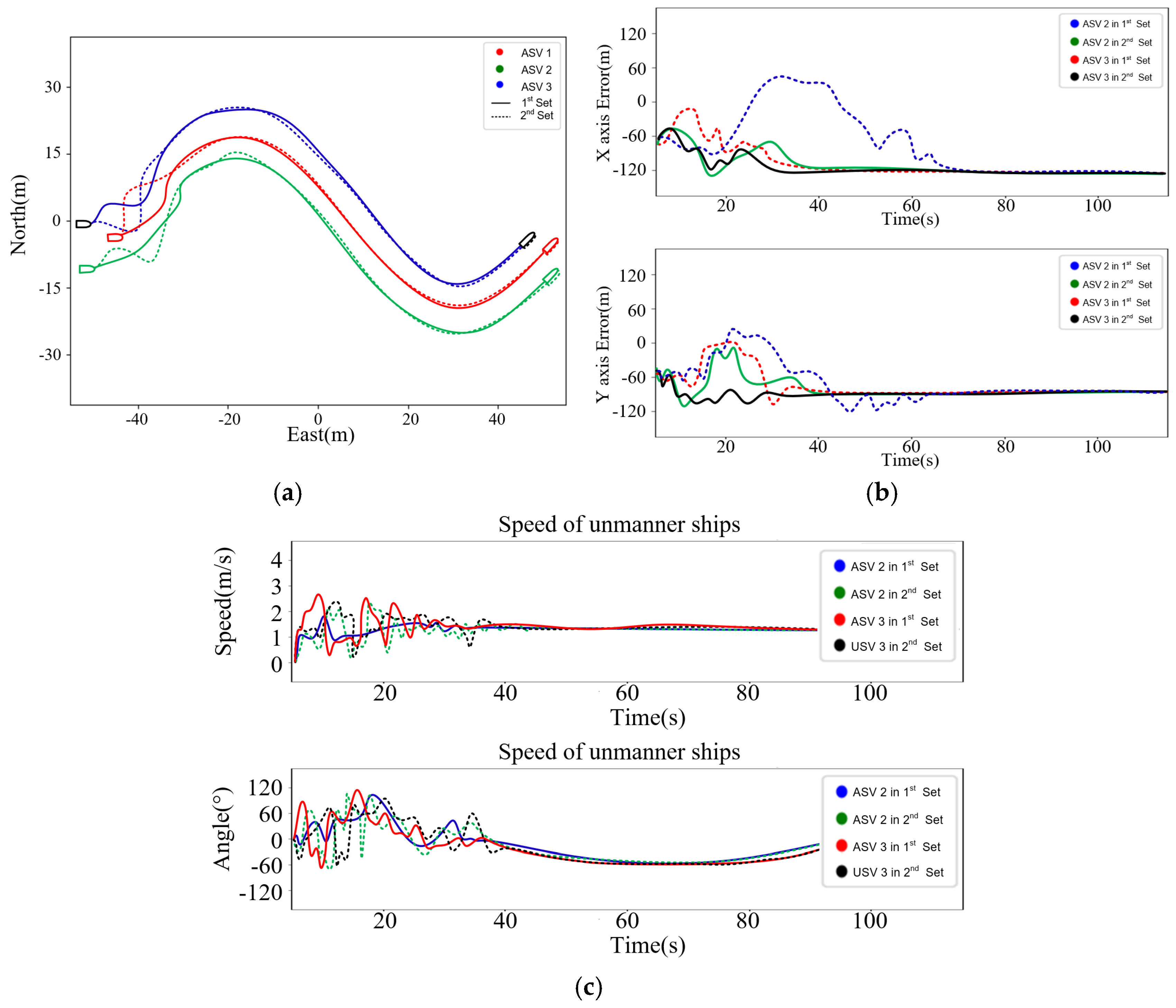
5.2.3. Case III: Sinusoidal Cooperative Formation Control

In this case, the cooperative formation control was tested under sinusoidal trajectory conditions. The goal was to evaluate how well the formation control could handle parameter changes. The effectiveness of the control effect under different parameter setting scenarios was analyzed using the sinusoidal trajectory as an example. Among them, Figure 11a shows the experimental results of the control method under different parameter setting scenarios, i.e., the effectiveness of ASV formation control under delays. The experimental results show that the first set of parameter settings had a better smoothing effect on the reference trajectory generation of the follower, while the smoothed desired trajectory affected the control effect of ASV formation. Combined with Figure 11b, it can be concluded that the desired trajectory smoothing process could effectively improve the convergence speed of the ASV formation. Figure 11c demonstrates the variation in the bow angle and speed of the following ship with different controllers. The experimental results demonstrate that the method proposed in this paper can effectively realize ship formation control and can handle the time delay disturbance.

6. Conclusions

This paper mainly studied the cooperative control strategy of ASV formations. Firstly, a separate state control strategy was designed based on the kinematic model of ships, which can control the speed and direction angle of ships within the formation to converge. Secondly, based on consistency theory, a control strategy for multiple ASV formations in ideal environments was designed, effectively enabling multiple ships to form and maintain a certain formation. Then, in response to the time delay problem that occurs during the formation of ships, a multi-ASV formation cooperative control strategy based on consistency theory under time delay conditions was designed, and the convergence and stability of the control strategy were proven using Lyapunov’s theorem. Finally, simulation verification was conducted on the proposed ASV formation cooperative control strategy. As a direction for future research, we plan to explore the interaction between autonomous vessels and human-operated vessels, particularly in cases where human operators deviate from expected behaviors or regulations. In addition, we will focus on incorporating additional environmental factors, such as ocean currents, and expanding the application scenarios of this method under different tasks.

References

1. Wen, Y.; Tao, W.; Sui, Z.; Piera, M.A.; Song, R. Dynamic model-based method for the analysis of ship behavior in marine traffic situation. Ocean Eng. 2022, 257, 111578. [Google Scholar] [CrossRef]
2. Du, B.; Xie, W.; Zhang, W.; Chen, H. A target tracking guidance for unmanned surface vehicles in the presence of obstacles. IEEE Trans. Intell. Transp. Syst. 2023, 25, 4102–4115. [Google Scholar] [CrossRef]
3. Zhang, M.; Du, L.; Wen, Y.; Guo, L.; Wu, B. Optimization of ship transport capacity structure for traffic congestion alleviation on inland waterways. Ocean Eng. 2024, 311, 118841. [Google Scholar] [CrossRef]
4. Granado, I.; Hernando, L.; Galparsoro, I.; Gabiña, G.; Groba, C.; Prellezo, R.; Fernandes, J.A. Towards a framework for fishing route optimization decision support systems: Review of the state-of-the-art and challenges. J. Clean. Prod. 2021, 320, 128661. [Google Scholar] [CrossRef]
5. Bae, I.; Hong, J. Survey on the developments of unmanned marine vehicles: Intelligence and cooperation. Sensors 2023, 23, 4643. [Google Scholar] [CrossRef]
6. Li, J.; Zhang, G.; Zhang, W.; Zhang, X. Robust control for cooperative path following of marine surface-air vehicles with a constrained inter-vehicles communication. Ocean Eng. 2024, 308, 118240. [Google Scholar] [CrossRef]
7. Tao, W.; Zhu, M.; Chen, S.; Cheng, X.; Wen, Y.; Zhang, W.; Negenborn, R.R.; Pang, Y. Coordination and optimization control framework for vessels platooning in inland waterborne transportation system. IEEE Trans. Intell. Transp. Syst. 2023, 24, 15667–15686. [Google Scholar] [CrossRef]
8. Peng, Z.; Wang, J.; Wang, D.; Han, Q.-L. An overview of recent advances in coordinated control of multiple autonomous surface vehicles. IEEE Trans. Ind. Inform. 2020, 17, 732–745. [Google Scholar] [CrossRef]
9. Jadbabaie, A.; Lin, J.; Morse, A. Coordination of Groups of Mobile Autonomous Agents Using Nearest Neighbor Rules. IEEE Trans. Autom. Control 2003, 48, 988–1001. [Google Scholar] [CrossRef]
10. Chung, S.J.; Paranjape, A.A.; Dames, P.; Shen, S.; Kumar, V. A Survey on Aerial Swarm Robotics. IEEE Trans. Robot. 2018, 34, 837–855. [Google Scholar] [CrossRef]
11. Bunic, M.; Bogdan, S. Potential Function Based Multi-Agent Formation Control in 3D Space. IFAC Proc. Vol. 2012, 45, 682–689. [Google Scholar] [CrossRef]
12. Chang, D.; Shadden, S.; Marsden, J.; Olfati-Saber, R. Collision Avoidance for Multiple Agent Systems. In Proceedings of the 42nd IEEE International Conference on Decision and Control, Maui, HI, USA, 9–12 December 2003. [Google Scholar]
13. Do, K. Formation Control of Mobile Agents Using Local Potential Functions. In Proceedings of the 2006 American Control Conference, Minneapolis, MN, USA, 14–16 June 2006. [Google Scholar]
14. Anh, D.; La, H.; Nguyen, T.; Horn, J. Formation Control for Autonomous Robots with Collision and Obstacle Avoidance Using a Rotational and Repulsive Force–Based Approach. Int. J. Adv. Robot. Syst. 2019, 16, 172988141984789. [Google Scholar]
15. Piet, B.; Ablak, M.; Strub, G.; Changey, S.; Petit, N. Experiments of High-Level Formation Flight of a Medium-Scaled Swarm of Micro UAVs in a Confined Environment with Obstacles. In Proceedings of the 2025 AIAA SciTech, Orlando, FL, USA, 6–10 January 2025. [Google Scholar]
16. Abbasi, M.; Marquez, H.J. Dynamic Event-Triggered Formation Control of Multi-Agent Systems With Non-Uniform Time-Varying Communication Delays. IEEE Trans. Autom. Sci. Eng. 2024; early access. [Google Scholar]
17. Lodhi, Z.A.; Zhang, K. Formation Control of Multi-agent Systems Over Directed Topologies: A Sliding Mode Control Approach With Prescribed-time Convergence. Int. J. Control Autom. Syst. 2024, 22, 3177–3190. [Google Scholar] [CrossRef]
18. Cao, X.; Li, K.; Li, Y. Robust adaptive formation control for nonlinear multi-agent systems with range constraints. Nonlinear Dyn. 2024, 112, 1917–1929. [Google Scholar] [CrossRef]
19. Epp, M.; Molinari, F.; Raisch, J. Exploiting Over-The-Air Consensus for Collision Avoidance and Formation Control in Multi-Agent Systems. arXiv 2024, arXiv:2403.14386. [Google Scholar]
20. Onuoha, O.; Kurawa, S.; Tang, Z.; Dong, Y. Discrete-time stress matrix-based formation control of general linear multi-agent systems. arXiv 2024, arXiv:2401.05083. [Google Scholar]
21. Moeurn, S.K. Distributed Cooperative Formation Control of Nonlinear Multi-Agent System (UGV) Using Neural Network. arXiv 2024, arXiv:2403.13473. [Google Scholar]
22. Liu, G.-P. Predictive control of networked nonlinear multiagent systems with communication constraints. IEEE Trans. Syst. Man Cybern. Syst. 2020, 50, 4447–4457. [Google Scholar] [CrossRef]
23. Zhang, D.-W.; Liu, G.-P.; Cao, L. Proportional integral predictive control of high order fully actuated networked multiagent systems with communication delays. IEEE Trans. Syst. Man Cybern. Syst. 2023, 53, 801–812. [Google Scholar] [CrossRef]
24. Psillakis, H.E. Adaptive NN cooperative control of unknown nonlinear multiagent systems with communication delays. IEEE Access 2021, 51, 5311–5321. [Google Scholar] [CrossRef]
25. Qi, T.; Lu, R.; Chen, J. Consensus of continuous-time multiagent systems via delayed output feedback: Delay versus connectivity. IEEE Trans. Autom. Control 2021, 66, 1329–1336. [Google Scholar] [CrossRef]
26. Pang, Z.H.; Luo, W.C.; Liu, G.P.; Han, Q.L. Observer-based incremental predictive control of networked multi-agent systems with random delays and packet dropouts. IEEE Trans. Circ. Syst. II Express Briefs 2021, 68, 426–430. [Google Scholar] [CrossRef]
27. Liu, G.P. Coordinated control of networked multiagent systems via distributed cloud computing using multistep state predictors. IEEE Trans. Cybern. 2022, 52, 810–820. [Google Scholar] [CrossRef] [PubMed]
28. Su, H.; Chen, J.; Chen, X.; He, H. Adaptive observer-based output regulation of multiagent systems with communication constraints. IEEE Trans. Cybern. 2021, 51, 5259–5268. [Google Scholar] [CrossRef]
29. Zhang, C.; Zhang, G.; Zhang, X. DVSL guidance-based composite neural path following control for underactuated cable-laying vessels using event-triggered inputs. Ocean Eng. 2021, 238, 109713. [Google Scholar] [CrossRef]
30. Chen, C.; Zou, W.; Xiang, Z. Event-triggered connectivity-preserving formation control of heterogeneous multiple USVs. IEEE Trans. Syst. Man Cybern. Syst. 2024, 54, 7746–7755. [Google Scholar] [CrossRef]
31. Chen, Y.; Guo, X.; Luo, G.; Liu, G. A formation control method for AUV group under communication delay. Front. Bioeng. Biotechnol. 2022, 10, 848641. [Google Scholar] [CrossRef]
32. Li, J.; Du, J.; Li, Y.; Xu, G. Distributed robust prescribed performance 3-D time-varying formation control of underactuated AUVs under input saturations and communication delays. IEEE J. Ocean. Eng. 2023, 48, 649–662. [Google Scholar] [CrossRef]
33. Li, J.; Tian, Z.; Zhang, H. Discrete-time AUV formation control with leader-following consensus under time-varying delays. Ocean Eng. 2023, 286, 115678. [Google Scholar] [CrossRef]
34. Sadeghzadeh-Nokhodberiz, N.; Meskin, N. Consensus-based distributed formation control of multi-quadcopter systems: Barrier Lyapunov function approach. IEEE Access 2023, 11, 142916–142930. [Google Scholar] [CrossRef]
35. Du, Z.; Qu, X.; Shi, J.; Lu, J. Formation control of fixed-wing UAVs with communication delay. ISA Trans. 2024, 146, 154–164. [Google Scholar] [CrossRef] [PubMed]
36. Liu, Y.; Bucknall, R. A survey of formation control and motion planning of multiple unmanned vehicles. Robotica 2018, 36, 1019–1047. [Google Scholar] [CrossRef]
37. Cui, Z.; Guan, W.; Zhang, X. ASV formation navigation decision-making through hybrid deep reinforcement learning using self-attention mechanism. Expert Syst. Appl. 2024, 256, 124906. [Google Scholar] [CrossRef]
38. Liu, H.; Weng, P.; Tian, X.; Mai, Q. Distributed adaptive fixed-time formation control for UAV-ASV heterogeneous multi-agent systems. Ocean Eng. 2023, 267, 113240. [Google Scholar] [CrossRef]
39. Lee, J.H.; Jeong, S.K.; Ji, D.H.; Park, H.Y.; Kim, D.Y.; Choo, K.B.; Jung, D.W.; Kim, M.J.; Oh, M.H.; Choi, H.S. Unmanned surface vehicle using a leader–follower swarm control algorithm. Appl. Sci. 2023, 13, 3120. [Google Scholar] [CrossRef]
40. Tan, G.; Zhuang, J.; Zou, J.; Wan, L. Coordination control for multiple autonomous surface vehicles using hybrid behavior-based method. Ocean Eng. 2021, 232, 109147. [Google Scholar] [CrossRef]
41. Wang, S.; Zhu, M.; Wen, Y.; Sun, W.; Zhang, W.; Lei, T. Formation tracking control for networked heterogeneous MSV systems with actuator faults: A distributed optimal event-triggered fixed-time sliding mode fault-tolerant control approach. Ocean Eng. 2024, 313, 119370. [Google Scholar] [CrossRef]
42. Chen, B.; Hu, J.; Zhao, Y.; Ghosh, B.K. Finite-time observer based tracking control of uncertain heterogeneous underwater vehicles using adaptive sliding mode approach. Neurocomputing 2022, 481, 322–332. [Google Scholar] [CrossRef]
43. Meng, C.; Zhang, W.; Du, X. Finite-time extended state observer based collision-free leaderless formation control of multiple AUVs via event-triggered control. Ocean Eng. 2023, 268, 113605. [Google Scholar] [CrossRef]
44. Fossen, T.I. Guidance and Control of Ocean Vehicles; Wiley: Hoboken, NJ, USA, 1999. [Google Scholar]
45. Wen, Y.; Tao, W.; Zhu, M.; Zhou, J.; Xiao, C. Characteristic model-based path following controller design for the unmanned surface vessel. Appl. Ocean Res. 2020, 101, 102293. [Google Scholar] [CrossRef]
Figure 1. Formation description under coordinate axis decomposition.
Jmse 13 00549 g001
Figure 2. Communication topology network of ship formations.
Jmse 13 00549 g002
Figure 3. Kinematics of dual-propulsion ship.
Jmse 13 00549 g003
Figure 4. Schematic diagram of multi-ship formation direction adjustment.
Jmse 13 00549 g004
Figure 5. Communication diagram and controller diagram of unmanned ships.
Jmse 13 00549 g005
Figure 6. Communication network structure considering delay.
Jmse 13 00549 g006
Figure 7. Block diagrams of proposed control strategies.
Jmse 13 00549 g007
Figure 8. The twin-propulsion ASV used for modeling in simulation experiments.
Jmse 13 00549 g008
Figure 9. Results of the experiment. (a) Results of formation trajectory; (b) results of error; (c) results of X direction; (d) results of Y direction.
Jmse 13 00549 g009
Figure 10. Results of cooperative control strategy under delays. (a) Results of formation trajectory; (b) results of heading angle; (c) experimental results of speed.
Jmse 13 00549 g010
Figure 11. Results of cooperative control strategy under different parameters. (a) Results of formation trajectory; (b) experimental results of error; (c) experimental results of heading angle and speed.
Jmse 13 00549 g011