Article

Impact of Coal-Fired Power Plants on Suspended Sediment Concentrations in Coastal Waters

1
Graduate Institute of Hydrological and Oceanic Sciences, National Central University, Taoyuan 320, Taiwan
2
Graduate Institute of Environmental Engineering, National Central University, Taoyuan 320, Taiwan
*
Author to whom correspondence should be addressed.
J. Mar. Sci. Eng. 2025, 13(3), 563; https://doi.org/10.3390/jmse13030563
Submission received: 3 February 2025 / Revised: 5 March 2025 / Accepted: 12 March 2025 / Published: 14 March 2025
(This article belongs to the Special Issue Coastal Hydrodynamic and Morphodynamic Processes)

Abstract

:
Many coastal coal-fired power plants utilize seawater flue gas desulfurization (SWFGD) systems, which may pose risks of heavy metal attachment on suspended sediments. Understanding variations in suspended sediment concentration (SSC) is therefore useful for controlling marine pollution. We studied two power plants as examples of discharging SSC using continuous measurement techniques. Monitoring sites at intake and discharge points and the surrounding coastal areas of the power plants was conducted across seasons. The first case study, Linkou Power Plant, is located in a high-SSC region influenced by monsoon winds and wave activity. Results indicate that SSC levels at all the monitoring sites are correlated with environmental factors of wind and wave conditions, with strong positive correlations observed between the intake and discharge points. In contrast, the Dalin Power Plant is located within an international harbor, where the SSC levels are generally low; however, sudden increases in SSC are observed at the intake point due to disturbances from vessel activities. These sudden increases are not evident at the discharge point, suggesting a sink of SSC may occur within the system. These results demonstrate that the two studied power plants have limited effects on the increase in SSC; the SSC in the discharge point is mainly related to the SSC input at the intake point. Effective management of SSC at the intake may help mitigate coastal pollution caused by SSC discharge and reduce the risk of harmful substances adhering to suspended solids in the discharging wastewater.

1. Introduction

Coal-fired power generation remains one of the central methods of electricity production worldwide. To reduce environmental challenges, power plants have adopted seawater flue gas desulfurization (SWFGD) systems to achieve desulfurization in reducing SO2 emissions [1,2,3,4]. However, the SWFGD systems pose some challenges, such as the release of mercury from coal into seawater. Consequently, research often focuses on the mercury content in the effluent of these systems [5,6,7]. Mercury tends to adsorb onto suspended sediments/solids (SSs), which can transport and spread over time [8,9,10]. If the SSs in the water of the intake are reduced, it is possible to decrease the attachment of pollutants on SSs [11]. Studies have shown that harmful heavy metals can adhere to SSs and are discharged along with wastewater from coal-fired power plants [12]. Coal combustion in power plants produces not only mercury but also SS, which can be found in the discharged wastewater [13]. Understanding variations in suspended sediment concentration (SSC) may help mitigate coastal pollution resulting from wastewater discharged by power plants.
Quantifying SSC is crucial for environmental monitoring and management [14,15]. SSC is a measure of the sediment weight concentration in water and serves as an important indicator for environmental regulation and sediment transport studies [16,17]. Many guidelines were reported as part of their regulations on controlling SSC because high or low SSC levels can harm the environment [18,19,20]. Consequently, standards for discharge SSC limits vary by country: Taiwan allows up to 30 mg/L, the European Union permits 10–30 mg/L, and the United States sets a single-day maximum of 100 mg/L and a 30-day average not exceeding 30 mg/L.
Traditionally, SSC measurement involved collecting on-site water samples and analysis in a laboratory [15,21,22]. This method, though accurate, is not suitable for continuous and long-term monitoring. OBSs have become prevalent for continuous SSC measurement [23]. The sensors are based on the linear relationship between near-infrared backscatter intensity and SSC, allowing the estimation of sediment concentrations [15]. However, OBS measurements can be affected by factors such as particle size and concentration; careful calibration is needed to obtain accurate measurements of SSC [15,23].
Factors influencing SSC include anthropogenic and natural environmental causes. Naturally, the resuspension and transport of SS are primarily driven by waves and cur-rents [24,25,26]. Sediments begin to move when the bed shear stress exceeds a critical threshold, which depends on sediment settling velocity, itself influenced by particle size [27,28]. In general, sediments move when bed shear stress exceeds the settling velocity and settle when the settling velocity is higher than the bed shear stress [29]. However, in coastal environments with artificial facilities, the hydrodynamic driving force and the sediment transport process are not as simple as in a purely natural environment. The coastal jetties, pumps, open channels, and facilities of the power plants complicate the hydrodynamics and sediment transport process and limit the study of the impacts of the SWFGD system.
This study examined two coal-fired power plants with SWFGD systems, using continuous monitoring at intake sites, discharge, and outfall and an environmental reference point to evaluate the influence of the entire waterflow system of the power plants on changes in SSC. The impact of the whole waterflow system of the power plants on SSC is therefore examined through the difference between the input (intake) and output (discharge) points. By analyzing SSC at input and output sites, this study assesses the variation of SSC and understands the factors influencing SSC at the monitoring sites.

2. Methods

2.1. Site Description

Two coal-fired power plants equipped with SWFGD systems were investigated to study the impact of SWFGD systems on the variation of SSC. The Linko power plant (LPP) and Dalin power plant (DPP) are located on the northern and southern sides of the Taiwan Strait, respectively, as shown in Figure 1a. The study area is in the subtropical monsoon region, influenced by the southwest monsoon in summer and the strong northeast monsoon in winter, resulting in temporal and spatial variability in marine meteorological conditions across the northern and southern sides of the strait [30,31,32]. High waves in the LPP during winter make it difficult to deploy and maintain the instruments; therefore, this study was conducted at the end of fall, at the onset of winter winds and waves. Field surveys across seasons were conducted for the two power plants: one in spring (LPP: 17 March to 29 March 2021; DPP: 26 February to 8 March 2021) and another in fall (LPP: 4 November to 29 November 2021; DPP: 21 October to 26 October 2021).
The suspension and transport of SSC in natural environments are primarily influenced by waves and currents [33,34]. Therefore, we collected tidal and wave data from tide stations and wave buoys deployed by the Marine Meteorology Center of the Central Weather Administration near each power plant. These included the Fugui Cape buoy (FC buoy), Zhuwei tide station (ZW tide station), Xiaoliuqiu tide station (XL tide station), and the Xiaoliuqiu buoy (XL buoy). The detailed locations of the tide stations and buoys are shown in Figure 1a.
Based on the annual statistical report on meteorological observation data for harbors and seas published by the Transportation Research Institute of the Ministry of Transportation and Communications in Taiwan, the monthly average wind speed in the LPP oceanic area ranges from 4.0 to 10.3 m/s, with average values of 5.8, 5.3, 7.0, and 10.3 m/s from spring to winter. The significant wave height (Hs) in the LPP varies across seasons, with average values of 0.88, 0.63, 1.19, and 1.46 m from spring to winter. In the DPP, the monthly average wind speed ranges from 2.1 to 2.9 m/s, with average values of 2.4, 2.3, 2.4, and 2.5 m/s from spring to winter. The wind speed and Hs in the DPP show relatively little variation across seasons, with the wave climate remaining mostly stable, except for some extreme typhoon waves in summer. The average significant wave height is 0.58, 1.04, 0.75, and 0.70 m from spring to winter.
In addition to the SWFGD system, other waterflow equipment includes seawater extraction equipment, pipes, circulating water channels, and aeration tanks; the seawater is then discharged back to the ocean through open channels. To understand the SWFGD system’s impact on SSC, we deployed instruments at S1 (intake), S1A (in-take), S2 (discharge), and S3 (outfall) points. Additionally, a survey site was established near the plant to assess the relationship between SSC in the surrounding marine area and the power plant. Figure 1b and Figure 1c illustrate the structural layout and survey points of the LPP and DPP, respectively. During the first survey at LPP, the intake point was positioned far from the seawater pump of the SWFGD system, resulting in a low correlation between SSC measurements at the intake and discharging points. Consequently, the second survey added a survey site near the seawater pump room. We designated the survey sites at each power plant as follows: the intake point is named S1, the discharging point is S2, the outfall point is S3, and the reference marine point is B1. An additional intake point near the seawater pump room was added during the second survey at LPP, as noted as S1A.
LPP is located on the northwest side of the Taiwan Strait, as shown in Figure 1. The water intake of the LPP is situated between two barriers, and the outer and larger breakwater for sheltering the coal unloading dock and the two jetties closer to the land is Lin-Kou Port. The coastlines on both the northern and southern sides of the LPP are sandy beaches. Satellite images have shown the presence of high SSC turbid plumes in the coastal waters in surf zones. In contrast, the DPP is located on the southwest side of the Taiwan Strait, as depicted in Figure 1. The water intake of the DPP is situated within Kaohsiung Port, an international commercial harbor; therefore, the water near the intake is relatively stable. Additionally, there are no significant sand sources in the waters surrounding DPP.

2.2. Suspended Sediment Concentration Measurements

The OBS instrument does not directly measure the weight of suspended particles in the water; instead, it measures the intensity of infrared light reflected by the SS. Therefore, careful calibration is required to accurately estimate the SSC from the OBS [15,23,35]. As each OBS probe may respond differently to various particle sizes and concentrations, we conducted individual calibrations for the OBS measurements at each survey point across different seasons. We collected water samples at each OBS site for calibration in the laboratory. The water depth of the water samples matched the vertical depth at which the OBS was deployed. A specialized water tank was used for calibration, as reported by Ly and Huang [15]. Linear regression relationships between the voltage readings from the OBS and SSC were established for the estimate of SSC. Detailed calibration results are shown in Appendix A, Table A1.
In this study, the OBSs were operated with a sampling rate of 2 Hz, recording for the first 2 min every hour. According to the results of the vertical profiles surveys, the total TVC and particle size distribution at both the intake and outfall were relatively uniform throughout the water column, except for some variations at the bottom and surface layers, as shown later. The TVC reflects a relation with SSC [36,37]. We sampled at a point 2 m from the surface and at another point at the mid-water depth for all surveys. The results showed that the measured values of SSC at the surface are similar to those at the point of mid-water depth. The mean water depths varied among the monitoring sites, and the measured depths also varied due to the tides (Appendix A, Table A1). As a result, we selected the data at mid-water depth as the representative. We tried to avoid biological attachment and human damage; equipment malfunctions still occurred during the field surveys, resulting in missing data for some monitoring sites, as shown in the discontinuity in the time series data.

2.3. Particle Size Distribution Measurement

The sediment size not only affects the estimation of SSC using OBS but also influences the sediment pick-up and suspension conditions [23,27,36,37]. This study employed the LISST 200X, which provides in situ particle size measurements ranging from 1 to 500 μm [38]. Background calibration using pure water was performed for the LISST before the field surveys [39]. In addition to measuring particle size distribution, the LISST 200X can also output the total volumetric concentration (TVC). Vertical profiles of particle size distributions were measured at the water intake and outfall of the two power plants (site S1 and S3), with vertical sampling positions conducted per meter intervals. Surveys were conducted during both the spring and fall seasons [40], and only one profile of flooding and ebbing tides was performed in each season to understand the effect from tides.

2.4. Heavy Metal Compositions of SS

We collected water samples for heavy metal composition analysis of SS at the intake and discharge points of the LPP (12 samples in spring and 6 in fall) and the DPP (12 samples in spring and 4 in fall). The samples were analyzed in accordance with the standard method NIEA M301.00B, as announced by the Environmental Analysis Laboratory of the Ministry of Environment. Water samples from the intake and discharge points were filtered using glass fiber filters (1.0 μm, Pall Corporation, Port Washington, NY, USA), followed by microwave digestion of the filters. The heavy metals, including arsenic, cadmium, chromium, copper, lead, nickel, and selenium, in the SS from both the intake and discharge points were then analyzed using inductively coupled plasma optical emission spectroscopy (ICP-OES, PerkinElmer/Avio 220 Max, Shelton, CT, USA).

3. Results

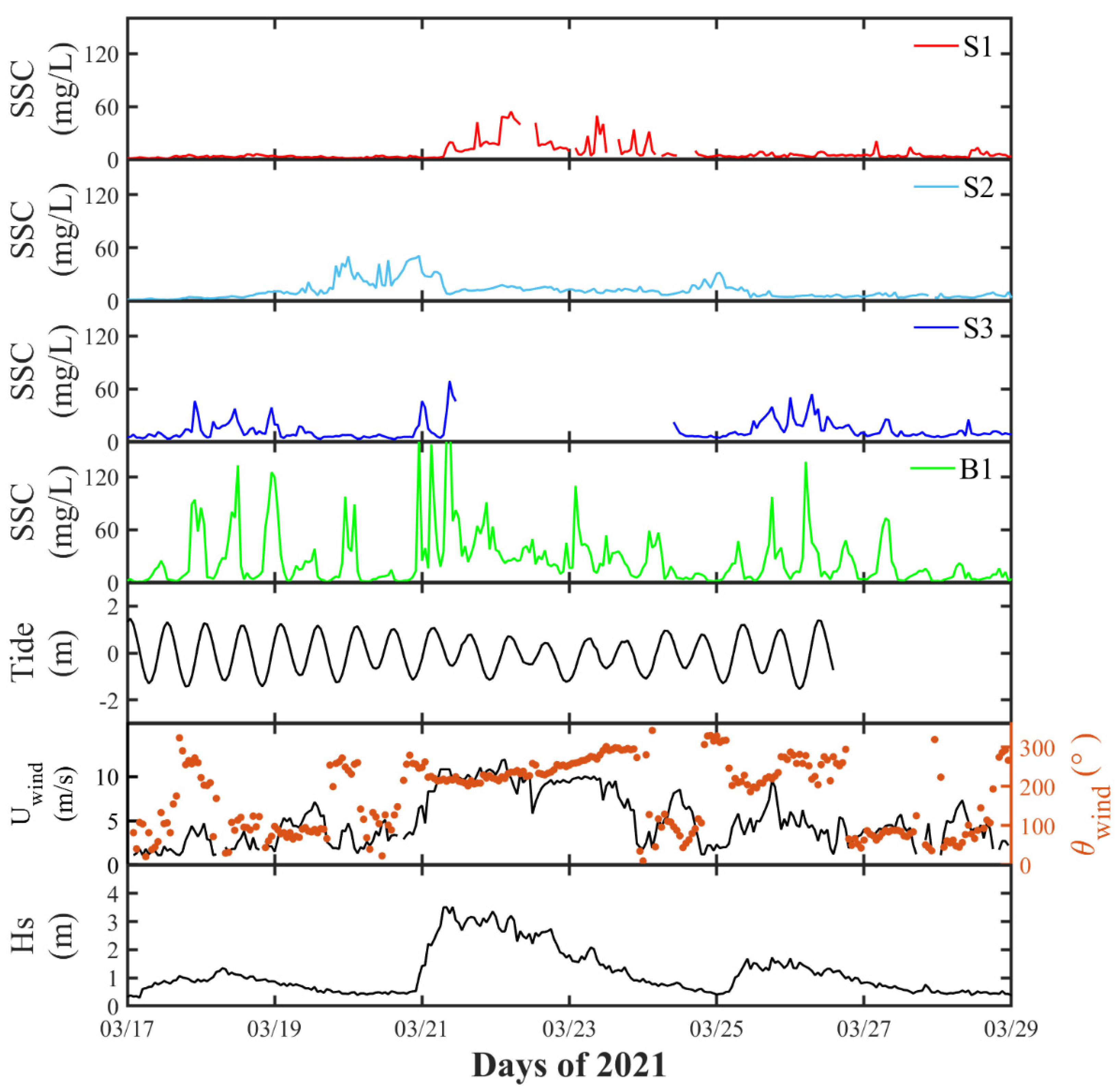
3.1. Linko Power Plant (LPP)

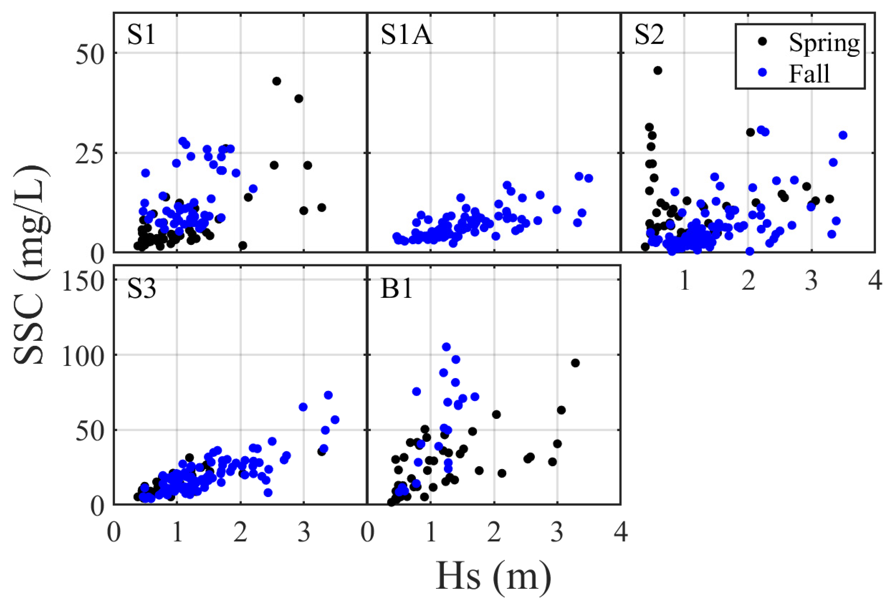
3.1.1. Variation of SSC

The results from the spring survey reveal that the temporal variations of SSC differ between locations S1 and S2 (Figure 2). This disparity is hypothesized to be related to the measurement locations, as the shape of the harbor in this area is complex. The waves are influenced by shielding and refraction effects, which may lead to variations in the hydrodynamics and turbulence at different measurement points, resulting in different SSC readings at those locations.
In addition, we found that there is no correlation in SSC measurements between sites S2, S3, and B1. The periods of high SSC values at S3 and B1 are similar, indicating that the SSC in the vicinity of the discharge point is more influenced by external environmental factors, such as wind and waves. From 21 March to 25 March, when significant wave heights exceeded 2 m, the SSC at sites S1 and B1 increased significantly, while S2, which is sheltered by the harbor, showed no significant change in SSC.
The spatial differences from S1 to the intake point may cause variations in SSC between these locations. Therefore, during the fall season, we established a new monitoring site called S1A near the seawater pump house. Figure 3 shows the temporal hourly data from the fall season survey. The observed SSC at S1A is lower than that at S1, which confirms that SSC variations are influenced by the spatial locations of the measurement points. Notably, there is a strong correlation in SSC between sites S1A and S2. In contrast, the SSC measured at site S3, located outside the discharge point, shows a higher correlation with wave conditions. Although the survey during the fall season at site B1 lasted only about five days, its SSC concentration and variation were significantly higher than those at other sites surrounding the power plant.

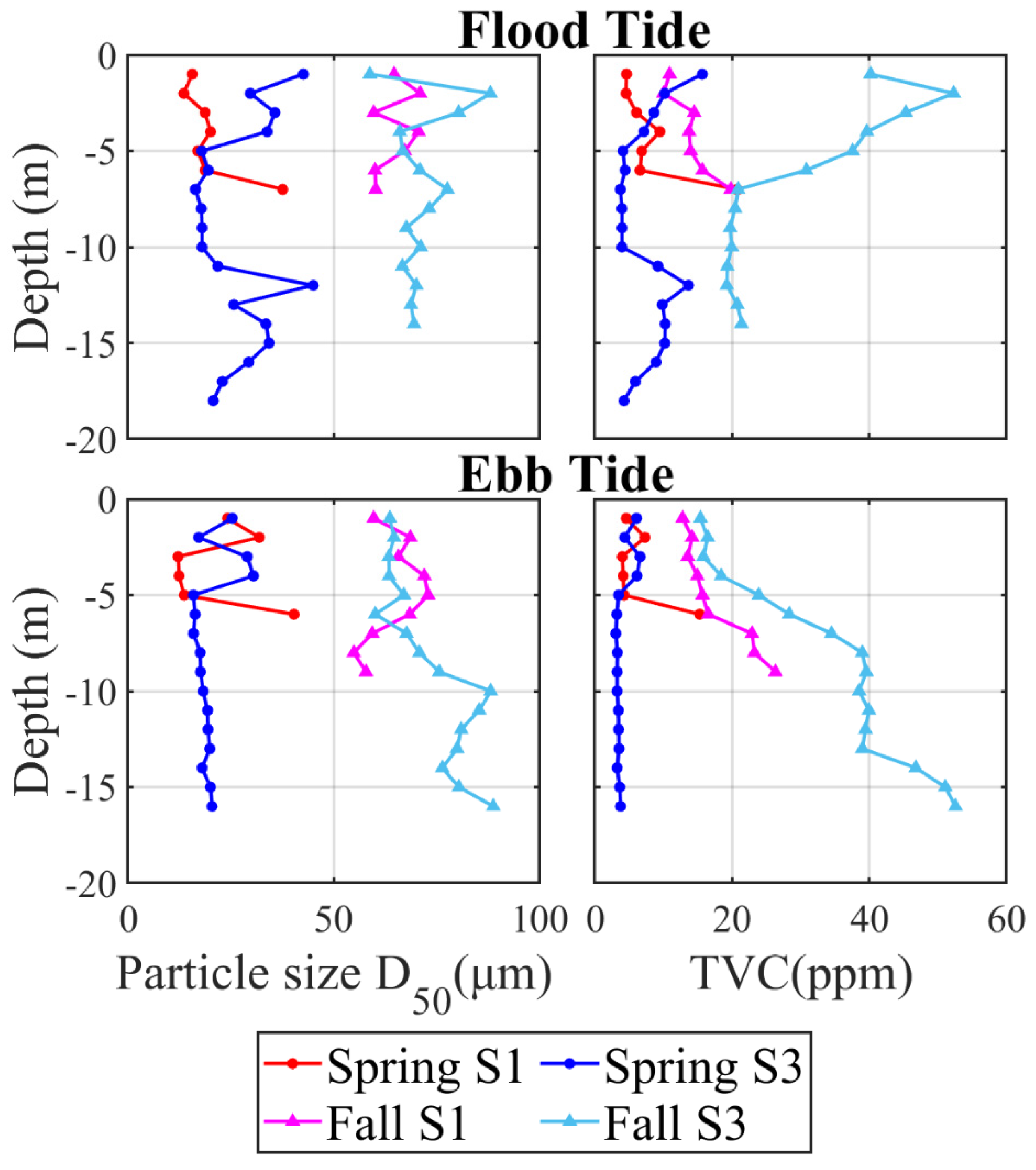
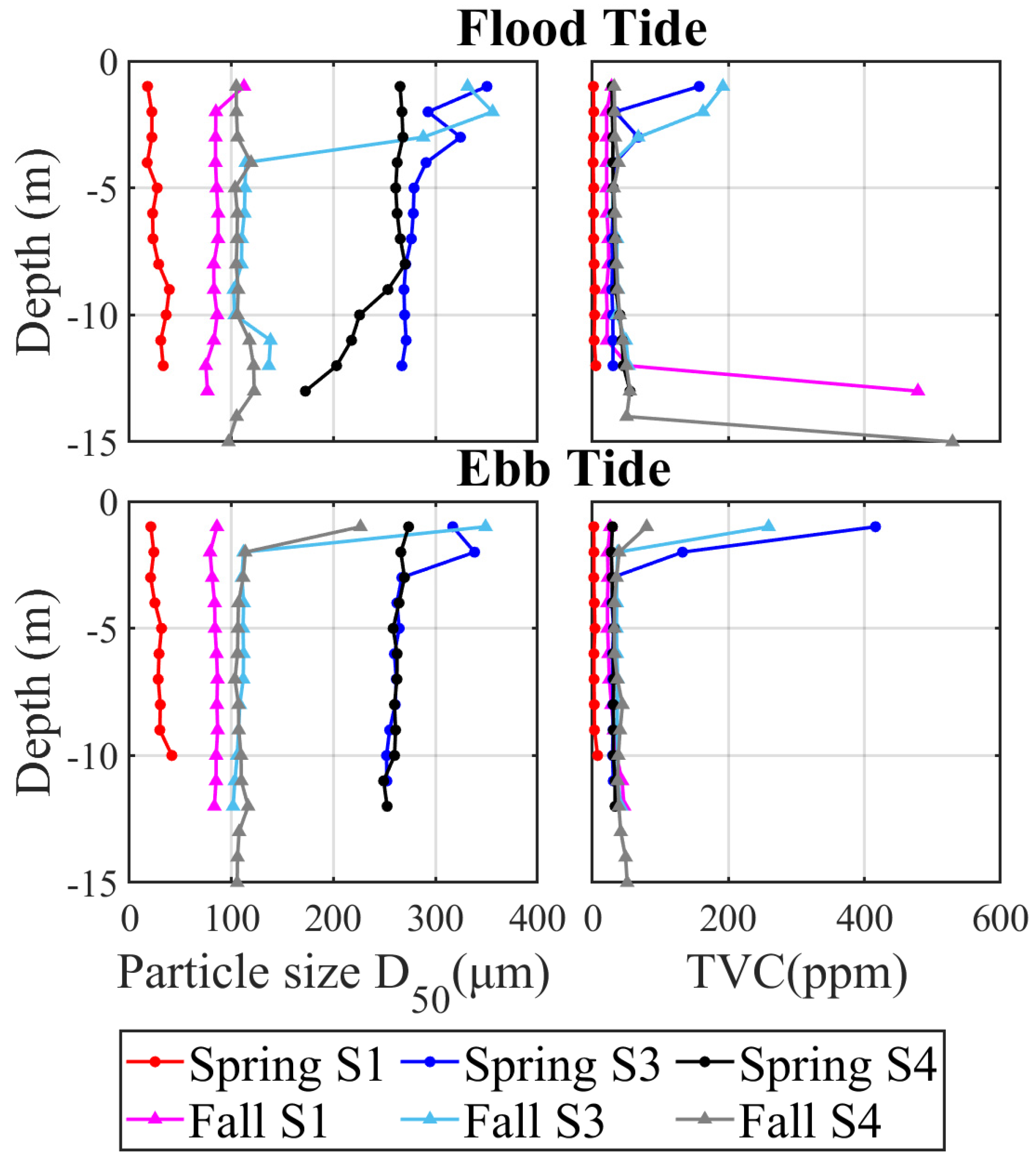
3.1.2. Particle Size and TVC

Figure 4 shows the results of the profiles of the particle size and TVC distribution at the LPP for two seasons. It can be observed that the median particle sizes (D50) for sites of S1 and S3 during both seasons show very similar distributions with water depth, and the data across the entire layer are relatively uniform, with no differences between spring and ebb tides. The D50 ranges from approximately 0 to 50 µm and from 50 to 100 µm during the spring and fall seasons, respectively. The average significant wave height in spring was 0.6 m, whereas it was 1 m in the fall season; the larger wave height leads to greater turbulent shear stress, resulting in larger SS particle sizes [29,37].
The TVC is quite uniform for the whole water column across seasons and tidal conditions at site S1, with values below 30 ppm, although the measured concentrations in the fall season are slightly greater than those measured in spring. At site S3, during the spring survey, the entire water column is also quite uniform, with TVC averaging below 20 ppm.
However, in the fall season survey, there is a noticeable increase in TVC, reaching up to around 60 ppm. Furthermore, at site S3, significant differences between tidal phases are observed in the fall season; during high tide, the upper water column exhibits higher TVC, while the lower water column shows lower concentration, and the opposite occurs during low tide, indicating that site S3 is influenced by the direction of the tidal currents.

3.2. Dalin Power Plant (DPP)

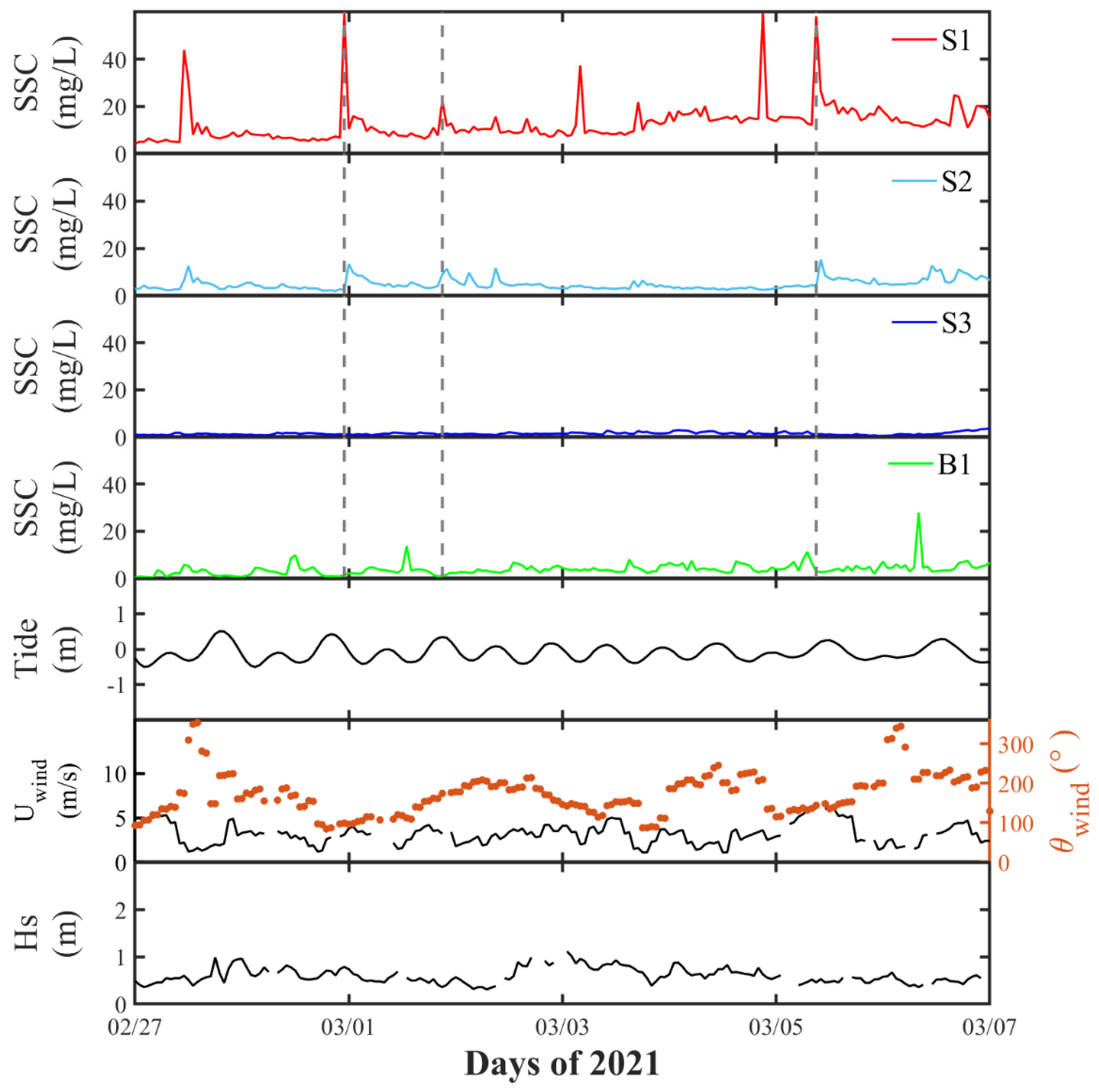
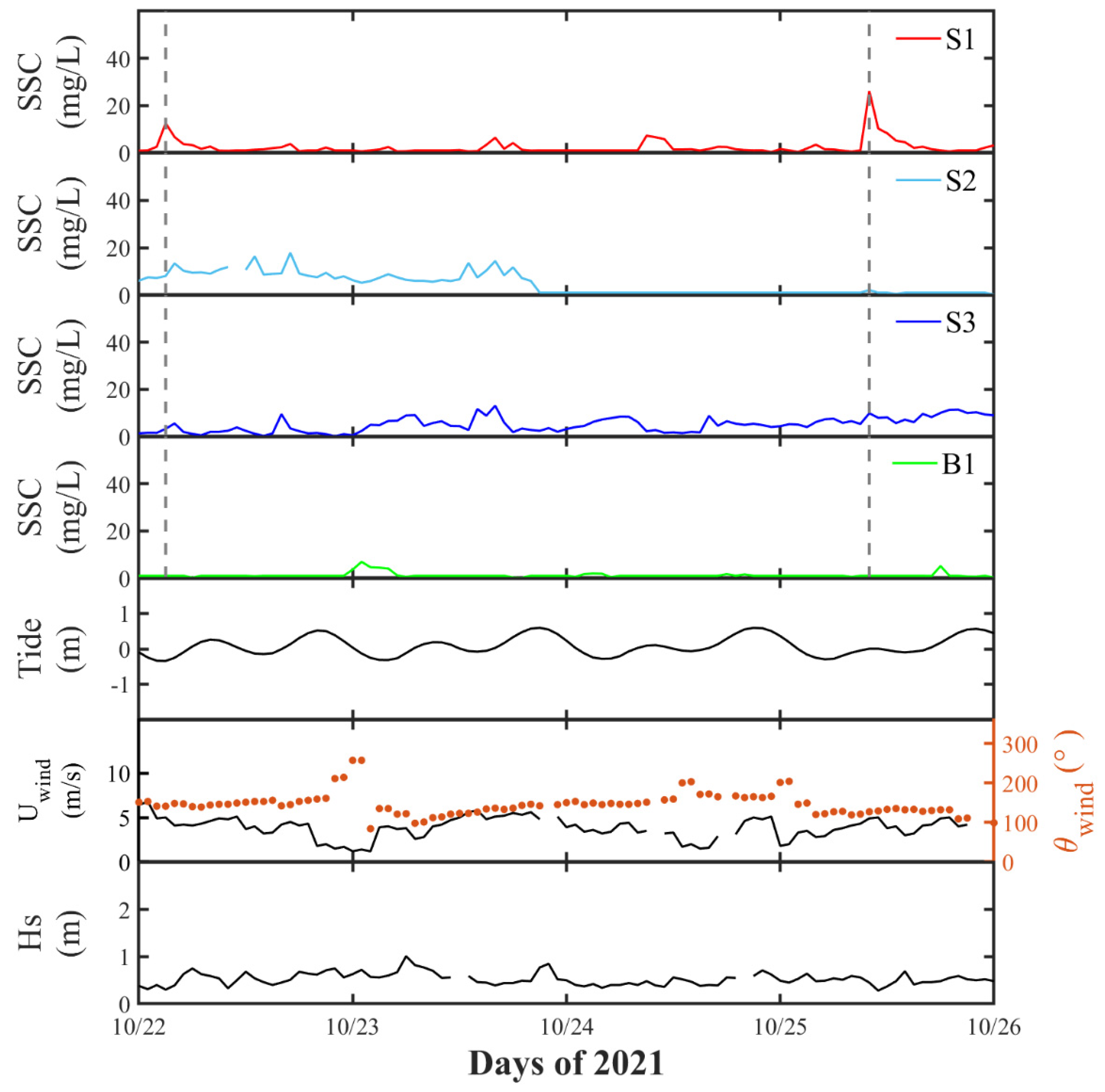
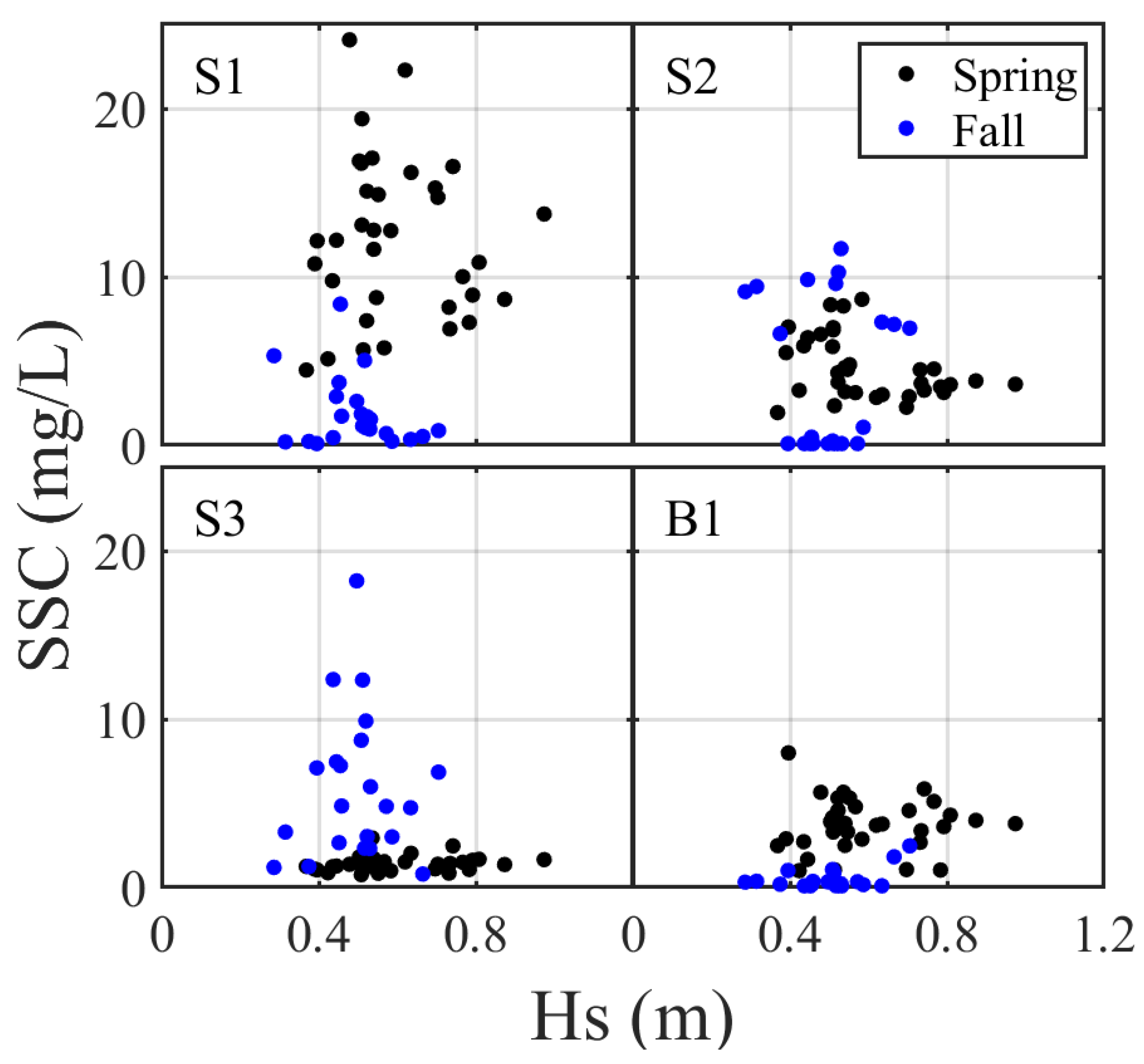
3.2.1. Variation of SSC

Figure 5 and Figure 6 present the time series results of SSC conducted at DPP during the spring and fall seasons; the observations in DPP begin two days before the end of the spring tide. The average significant wave heights during the survey periods for spring and fall were 0.6 m and 0.49 m, respectively. The SSC measurements from the four survey points were all lower than those recorded at LPP, with average concentrations less than 12 mg/L. Sudden increases in SSC are observed at the intake point. However, these increases are not evident at the discharge point. These SSC spikes, lasting only 1–2 h, with peak values occurring simultaneously, are observed for both seasons at the intake point (S1) and discharge point (S2). These sudden increases in SSC are attributed to disturbances caused by vessels at the intake point. In contrast, such increases are not observed at the outfall point (S3), indicating that sedimentation processes (the sink of SSC) may take place within the system.
The trend of the time series of SSC at the nearby environmental reference site B1 was different from those at S1 and S2, suggesting that the SSC inside surrounding coastal waters may not be significantly affected by the discharge water from DPP. In such a location with a distinct flow environment close to the open sea, SSC should be influenced by localized turbulence and resuspension effects [37,40].

3.2.2. Particle Size and TVC

Figure 7 shows the profile survey results of particle size and TVC at DPP for both seasons. At site S1, the D50 distribution trends in both spring and fall seasons vary similarly with depth, exhibiting a uniform distribution throughout the water column. In spring, the D50 range is approximately 0–50 µm, while in the fall season, it increases to 50–100 µm. At site S3, larger D50 values in the upper layer of the water column were observed for both seasons, with values ranging from approximately 275 to 350 µm. The D50 to the bottom measured around 250 to 275 µm in spring and about 100 to 150 µm in the fall season.
At site B1 during spring high tide, the D50 distribution is uniform from the surface to 8 m below, approximately 250–275 µm. Below 8 m, the D50 decreases gradually with depth, reaching about 175 µm at the bottom. During spring low tide, the D50 distribution remains uniform throughout the water column, around 250 to 275 µm. In the fall season, the particle size distribution at site S4 resembles that of S3, with a larger D50 in the surface layer, but the distribution becomes uniform below 2 m, ranging from approximately 100 to 150 µm.
The data are evident that the particle size at S1 is significantly smaller than that at S3. The result reflected the difference in the site location in Kaohsiung Harbor. The TVC at site S1 exhibits remarkably uniform values across both seasons and tidal conditions, consistently below 50 ppm, although there is a greater TVC near the bottom. A higher TVC is observed in the upper layers of the water column at sites S3 and B1 (>79 mg/L), while the TVC remains relatively uniform at approximately 50 ppm or below from 1 to 2 m below the surface.

4. Discussion

4.1. Analysis of Heavy Metal Compositions of SSs

The results of heavy metal compositions for collected SSs in the cases of LPP and DPP are summarized in Table 1. The data indicate that in the LPP case, higher concentrations of heavy metals such as Cr, Cu, Ni, and Se are observed at the discharge point compared to the intake point. In the DPP case, As and Se also show elevated concentrations at the discharge point. In contrast, Pb and Cd exhibit slightly lower concentrations in samples from the discharge point than in those from the intake point for the two power plants. Notably, measurements in fall are significantly higher than those in spring. These findings align with previous research indicating that heavy metals may adhere to SSs and be discharged along with wastewater from coal-fired power plants [6,12,13]. However, the data for the heavy metal analysis in the present study are relatively limited. Future studies that focus on quantifying the potential increase in heavy metals due to adhesion between the inlet and discharge sites are needed.
Elevated SSC levels can enhance the transport potential of heavy metals in aquatic environments [13]. However, water quality guidelines in Taiwan specify separate limits for SSC and heavy metal concentrations in seawater, without official standards for the attachment of heavy metals to SSC. This lack of regulation complicates the determination of harmful SSC levels in relation to metal content. Harmful levels of SSC may vary depending on specific environmental conditions and the types of metals involved. Notably, as SSC increases, the total mass of attached heavy metals is likely to rise. In our study, observations from the LPP case revealed a significant increase in heavy metal levels near the discharge point, whereas the DPP case exhibited minimal change. The differences between the two cases highlight variations in local SSC, pollution control within the power plant, and environmental backgrounds. The quantities of heavy metals attached to SSs detected in this study were minimal and significantly below the heavy metal concentrations in the water quality guidelines in Taiwan. Certain heavy metals were even below detectable levels (N.D.). Consequently, determining the SSC levels containing heavy metals that pose an environmental threat remains a critical area for future research, with the aim of developing more precise assessment criteria.

4.2. Factors Affecting the Variation of SSC

The S3 and B1 sites are similar in spring but show different patterns in fall. The reason may be attributed to the complex interaction between local hydrodynamics (wind, waves, current) and the harbor’s shape [41]. Wind speed is higher in fall than in spring, and the water depth at S3 is greater than that at B1. This could lead to increased mixing and drifting currents that transport SSs from the upstream region to the shallow site of B1 in fall, resulting in higher SS values, as shown in Figure 3, whereas only a brief period of high wind speed occurred between 21 March and 22 March in spring, as illustrated in Figure 2. Figure 6 (fall) indicates a stable SSC trend at the B1 site, showing no correlation with other stations. In contrast, Figure 5 (spring) reveals that the SSC at the B1 site resembles the shape of that at S2. These two results in DPP are likely due to seasonal variations in wind and wave conditions. These results from LPP and DPP demonstrate that SSC is significantly influenced by local suspension conditions and hydrodynamic transport, resulting in spatial variability. Because field observations are often limited in their ability to represent comprehensive spatial differences, future studies could utilize numerical model data to address the limitations of point measurements in field observations [25].
The concentration and particle size distribution of SSs in water are primarily influenced by turbulence and the settling velocity of the sediments themselves. In flow regimes dominated by bottom boundary layers, the profile of SSC can be explained by Rouse’s theory [37,42,43]. However, in complex coastal environments, the movement and dynamics of the boundary layer are affected by driving forces and interactions such as waves, mean flows, and winds [25,44], complicating the turbulence generation. Other mechanisms (e.g., rainfall [45]) that affect turbulence production will consequently impact the physical properties of SSs. In coastal environments, wave-induced bed shear stress is often considered the dominant contributor; therefore, many studies have identified wave height as the most directly related physical parameter affecting SSC variations [15,26].
To reduce the interference of short-term fluctuations on data analysis, we averaged the SSC data every 6 h and computed the correlation coefficients with physical parameters of tides, waves, and wind speeds. The choice of a 6 h average is due to the dominance of semi-diurnal tide in the study site [30,46]. Except for site B1 in DPP, which has a correlation coefficient of −0.5, there is no significant correlation between SSC and tidal water levels at the other monitoring sites. The correlation coefficients between tidal levels and SSC range from −0.3 to −0.2. We found that the SSC at both power plants exhibited a higher correlation with significant wave height, as shown in Figure 8 and Figure 9.
The correlation coefficients of SSC with representative wave heights for the LPP for the data combing from the two seasons for sites of S1, S1A, S3, and B1 are all above 0.5, with S3 exhibiting a particularly high correlation coefficient of 0.86, indicating a significant influence of waves on the SSC. In contrast, the correlation coefficient for S2 is only 0.29. This discrepancy is possibly attributed to some data in spring, in which a notable increase in SSC on two occasions (19 to 21 March and 24 to 26 March) occurred at site S2. However, the wave heights during the two occasions were all below 1 m, indicating other factors may have contributed to the rise in SSC. If we analyze the data in fall alone, the correlation coefficient increases to 0.64. In the study, we found a notable result that the correlation coefficient between sites S2 and S1A is 0.91, where S2 and S1A are monitoring sites within and outside the power plant. This indicates a strong relationship between the SSC within and outside the power plant.
The correlation of SSC at the four monitoring sites for the DPP with data for wind, wave, and tide is low, with correlation coefficients ranging between −0.2 and 0.2, as shown in Figure 9. However, sudden increases in SSC are observed at the intake point (site S1) due to vessel activity. When vessels approach, the SSC concentration, initially below 10 mg/L, can suddenly rise to over 20 mg/L, indicating that vessel movement has a significant impact on the SSC in that area. We cannot fully capture all vessel passages at site S1, but we recorded the activity of the coal unloading ships for the power plant. We found that when coal unloading ships arrived at the port (as indicated by the gray dashed lines in Figure 5 and Figure 6), there was a rapid increase (like spikes) in SSC at site S1. The corresponding occurrence of the spikes is observed for SSC data at site S2. However, these sudden changes in SSC were not observed in sites S3 and S4.
The median grain size of the deposited sediment near the intake of DPP is very small (D50 = 14.8 µm), ranging in mud category. This is because the water body near the intake of DPP is relatively stable and not significantly affected by wind and waves. The resuspension of fine sediment could be anticipated due to the flow disturbance from the vessel activity. In contrast, sites S3 and B1 are in open sea areas, where the flow is comparatively easily affected by waves and currents, making the measured particle sizes (D50 = 150.3 µm) much larger at sites S3 and B1.

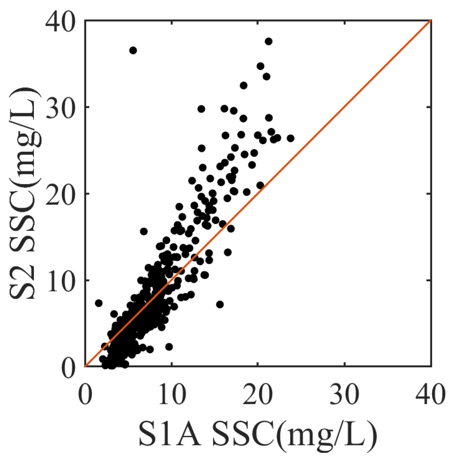
4.3. Change in SSC Between the Intake and Discharge Points

The extracted seawater enters the power plant through the intake points (S1, S1A) and then flows to the discharge point (S2) before being released into the outfall (S3). This study aims to investigate whether the whole system within the power plant increases or decreases SSC. We compute the differences in SSC obtained from the intake points (S1, S1A) and the discharge point (S2). Because the OBSs have been well calibrated and the accuracy of the OBS is less than 4%, the differences in SSC values between the inflow and outflow should allow the elimination of possible system errors, thereby allowing us to examine the change in SSC due to the impact of the power plant systems.
The data distribution analysis for one-to-one correlation is conducted only for the LPP data because the SSC values in the DPP are relatively low and primarily affected by sudden ship activities, which makes it difficult to exhibit continuous change characteristics in the one-to-one scatter plot. The correlation coefficient of SSC at sites S1 and S1A at the LPP is 0.62, suggesting that variations in spatial positioning can lead to differing SSC changes [8]. Remarkedly, a significant correlation between the SSC values at S1A and S2 is observed, with a correlation coefficient reaching 0.91, as shown in Figure 10. The change in SSC from the discharge point (S2) to the intake point (S1A) is approximately ±10 mg/L, with an average variation of 0.03 mg/L, indicating a minor change from the intake to the discharge point of the power plant. Furthermore, we found that when the SSC at S1A is below 10 mg/L, the average variation is −0.9 mg/L. In contrast, when the SSC at S1A exceeds 10 mg/L, the average variation increases to 3.9 mg/L. This result suggests that when seawater with lower concentrations enters the SWFGD system, there is a slight decrease in SSC. Conversely, seawater with a higher SSC entering the power plant would result in an increase in SSC at the discharge point. We hypothesize that this may be related to the packing material in the flue gas desulfurization tower; when the turbidity or flow rate of the incoming water is high, solid particles on the packing material may be washed out, leading to an increase in SSC observed in the discharge point. Further study may be needed to study the possible variation inside the power plant. Additionally, the change in SSC between S1A and S3 ranges from −8.3 to 104 mg/L, with the variation between S1A and S3 being significantly greater than that between S1A and S2.
At the DPP, the correlation coefficient of SSC between sites S1 and S2 is low (r < 0.2) for both seasons, primarily due to generally low SSC levels, mostly under 10 mg/L. This may be due to a similar reason as observed at the LPP; the site S1 is far from the actual intake point (S1A) of the power plant. However, the time series data still reveal a noticeable increase in SSC at the DPP when disturbances from vessels occur at the intake point, which subsequently affects the SSC at the discharge point. The overall change in SSC for both seasons is approximately ±10 mg/L, with an average variation of −1.4 mg/L. The result indicates that the impact of the power plant on SSC increases is relatively small, which aligns with the findings from the case of LPP.

5. Conclusions

This study uses two coal-fired power plants equipped with SWFGD systems as case studies, employing continuous monitoring methods at sites of intake (S1, S1A), discharge (S2), and outfall (S3) and an environmental reference point (B1) to assess the impact of the entire waterflow system of the power plant on variations in SSC. The field studies encompass two different seasons and two different marine areas. The marine environments at the intake and outfall points of the two power plants differ significantly. LPP is located near a beach and is surrounded by a breakwater, while DPP is situated within an international commercial harbor.
Profile measurements indicated a uniform vertical distribution of grain size and concentration on SSs. However, continuous SSC measurements reveal that SSC values exhibit spatial and temporal variations. The results suggest that the characteristics of local SS are influenced by changes in hydrodynamics at specific locations [25,37,40,41]. In the case of LPP, the variations in SSC at the intake points (S1, S1A), discharge point (S3), and nearby environmental reference site (B1) are notably affected by wave actions. In contrast, the SSC levels were low in coastal waters near the DPP across all monitoring sites. Sudden increases in SSC were noticeably observed due to vessel activity at the intake (S1) and discharge points (S2), whereas these sudden increases were not found at the outfall (S3) and the nearby reference site (B1). This also reflects that the local SSs are subject to the local hydrodynamics based on their spatial position.
The results showed that heavy metals may adhere to SSs and be discharged along with wastewater from coal-fired power plants. Elevated SSC levels can enhance the transport potential of heavy metals in aquatic environments [13]. Our results from the LPP indicate that as SSC increases, the total mass of attached heavy metals rises; however, the increase in heavy metals in the DPP case is not evident. This indicates that variations in local SSC, pollution control within the power plant, environmental backgrounds, and other factors complicate the attachment of heavy metals to SSs. Future studies to determine the SSC levels containing heavy metals that pose an environmental threat are needed.
Apart from the high SSC events during vessel activities, SSC levels in the DPP are generally low (mostly under 10 mg/L), making it difficult to differentiate the SSC between the intake and discharge points. However, a decrease in SSC from the intake to the discharge point can be observed during vessel activities. Additionally, the SSC at the discharge point (S2) of the LPP is strongly correlated (r = 0.91) with the SSC at the intake point. The analysis of the variations in SSC between the intake and discharge point reveals that the changes are small, less than approximately ±10 mg/L, while environmental factors can lead to SSC variations that are several times greater. These findings from both the power plants suggest that the SWFGD and the whole seawater flow systems have a limited impact on increasing SSC; the changes in discharging SSC out of the power plants are directly related to the SSC levels in the seawater being input. This result indicates that controlling the SSC at the intake of seawater could reduce the risk of heavy metal attachment to SSs in the SWFGD system, thereby mitigating the spread of coastal pollution.

Author Contributions

Z.-C.H. and P.-C.L. conducted the field surveys and prepared and revised the manuscript. Z.-C.H., P.-H.L. and S.-H.C. co-supervised the original research project and contributed to the manuscript revisions. All authors have read and agreed to the published version of the manuscript.

Funding

The data were obtained from the related project supported by TPC. ZCH received funding from the National Science and Technology Council in Taiwan under grant number NSTC 112-2621-M-008-004.

Institutional Review Board Statement

Not applicable.

Informed Consent Statement

Not applicable.

Data Availability Statement

The data presented in this study are available on request from the corresponding author.

Acknowledgments

ZCH was supported by the National Science and Technology Council in Taiwan under grant number NSTC 112-2621-M-008-004. We thank TPC for their support in research funds from related projects. The authors would like to thank the three anonymous reviewers for their comments, which have greatly improved the paper.

Conflicts of Interest

The authors declare no conflicts of interest.

Appendix A. Calibration of OBS

The OBSs used were carefully calibrated using the method reported by Ly and Huang [15]. Linear regression relationships between the voltage readings from the OBS and SSC were established for the estimate of SSC, as shown in Table A1.
Table A1. The average water depth data for each site, with the calibration parameters used to linearly convert OBS data (with units in mV) to suspended sediment concentration (SSC).
Linko Power Plant (LPP)
SeasonSpringFall
Dates 2021/03/17~2021/03/292021/11/05~2021/11/30
Depth (m)Calibration Equations (mg/L)Depth (m)Calibration Equations (mg/L)
S1~8 mSSC = 0.11 mV − 2.32~8 mSSC = 0.14 mV − 4.29
S1A ~8 mSSC = 0.09 mV − 2.44
S2~16 mSSC = 0.08 mV − 1.6~16 mSSC = 0.12 mV − 9.79
S3~24 mSSC = 0.12 mV − 0.15~24 mSSC = 0.09 mV − 4.45
B1~16 mSSC = 0.17 mV − 3.31~16 mSSC = 0.17 mV + 0.58
Dalin Power Plant (DPP)
Season SpringFall
Dates2021/02/27~2021/03/072021/10/22~2021/10/26
Depth (m)Calibration Equations (mg/L)Depth (m)Calibration Equations (mg/L)
S1~12 mSSC = 0.12 mV − 0.36~12 mSSC = 0.11 mV − 1.30
S2~5 mSSC = 0.10 mV − 2.3~5 mSSC = 0.09 mV − 8.53
S3~12 mSSC = 0.07 mV − 0.81~12 mSSC = 0.13 mV − 3.12
B1~13 mSSC = 0.20 mV − 3.75~13 mSSC = 0.09 mV − 3.04

References

  1. Oikawa, K.; Yongsiri, C.; Takeda, K.; Harimoto, T. Seawater flue gas desulfurization: Its technical implications and performance results. Environ. Prog. 2003, 22, 67–73. [Google Scholar] [CrossRef]
  2. Tokumura, M.; Baba, M.; Znad, H.T.; Kawase, Y.; Yongsiri, C.; Takeda, K. Neutralization of the acidified seawater effluent from the flue gas desulfurization process: Experimental investigation, dynamic modeling, and simulation. Ind. Eng. Chem. Res. 2006, 45, 6339–6348. [Google Scholar] [CrossRef]
  3. Duan, L.B.; Cui, J.; Jiang, Y.; Zhao, C.S.; Anthony, E.J. Partitioning behavior of Arsenic in circulating fluidized bed boilers co-firing petroleum coke and coal. Fuel Process. Technol. 2017, 166, 107–114. [Google Scholar] [CrossRef]
  4. Zhao, M.J.; Xue, P.; Liu, J.J.; Liao, J.H.; Guo, J.M. A review of removing SO2 and NOX by wet scrubbing. Sustain. Energy Technol. Assess. 2021, 47, 101451. [Google Scholar] [CrossRef]
  5. Liu, X.Y.; Sun, L.M.; Yuan, D.X.; Yin, L.Q.; Chen, J.S.; Liu, Y.X.; Liu, C.Y.; Liang, Y.; Lin, F.F. Mercury distribution in seawater discharged from a coal-fired power plant equipped with a seawater flue gas desulfurization system. Environ. Sci. Pollut. Res. 2011, 18, 1324–1332. [Google Scholar] [CrossRef]
  6. Sun, L.M.; Feng, L.F.; Yuan, D.X.; Lin, S.S.; Huang, S.Y.; Gao, L.M.; Zhu, Y. The extent of the influence and flux estimation of volatile mercury from the aeration pool in a typical coal-fired power plant equipped with a seawater flue gas desulfurization system. Sci. Total Environ. 2013, 444, 559–564. [Google Scholar] [CrossRef]
  7. Lin, H.Y.; Peng, J.J.; Yuan, D.X.; Lu, B.Y.; Lin, K.N.; Huang, S.Y. Mercury isotope signatures of seawater discharged from a coal-fired power plant equipped with a seawater flue gas desulfurization system. Environ. Pollut. 2016, 214, 822–830. [Google Scholar] [CrossRef]
  8. Schoellhamer, D.H.; Mumley, T.E.; Leatherbarrow, J.E. Suspended sediment and sediment-associated contaminants in San Francisco Bay. Environ. Res. 2007, 105, 119–131. [Google Scholar] [CrossRef]
  9. Flanders, J.R.; Turner, R.R.; Morrison, T.; Jensen, R.; Pizzuto, J.; Skalak, K.; Stahl, R. Distribution, behavior, and transport of inorganic and methylmercury in a high gradient stream. Appl. Geochem. 2010, 25, 1756–1769. [Google Scholar] [CrossRef]
  10. Pizzuto, J.E. Long-term storage and transport length scale of fine sediment: Analysis of a mercury release into a river. Geophys. Res. Lett. 2014, 41, 5875–5882. [Google Scholar] [CrossRef]
  11. Lu, F.; Zhang, H.Q.; Jia, Y.G.; Liu, W.Q.; Wang, H. Migration and Diffusion of Heavy Metal Cu from the Interior of Sediment during Wave-Induced Sediment Liquefaction Process. J. Mar. Sci. Eng. 2019, 7, 449. [Google Scholar] [CrossRef]
  12. Peterson, R.N.; Burnett, W.C.; Opsahl, S.P.; Santos, I.R.; Misra, S.; Froelich, P.N. Tracking suspended particle transport via radium isotopes (226Ra and 228Ra) through the Apalachicola-Chattahoochee-Flint River system. J. Environ. Radioact. 2013, 116, 65–75. [Google Scholar] [CrossRef]
  13. Sun, L.M.; Lin, S.S.; Feng, L.F.; Huang, S.Y.; Yuan, D.X. The distribution and sea-air transfer of volatile mercury in waste post-desulfurization seawater discharged from a coal-fired power plant. Environ. Sci. Pollut. Res. 2013, 20, 6191–6200. [Google Scholar] [CrossRef] [PubMed]
  14. Pearson, S.G.; Verney, R.; van Prooijen, B.C.; Tran, D.; Hendriks, E.C.M.; Jacquet, M.; Wang, Z.B. Characterizing the Composition of Sand and Mud Suspensions in Coastal and Estuarine Environments Using Combined Optical and Acoustic Measurements. J. Geophys. Res.-Ocean. 2021, 126, e2021JC017354. [Google Scholar] [CrossRef]
  15. Ly, T.N.; Huang, Z.C. Real-time and long-term monitoring of waves and suspended sediment concentrations over an intertidal algal reef. Environ. Monit. Assess. 2022, 194, 839. [Google Scholar] [CrossRef] [PubMed]
  16. Schoellhamer, D.H. Variability of suspended-sediment concentration at tidal to annual time scales in San Francisco Bay, USA. Cont. Shelf Res. 2002, 22, 1857–1866. [Google Scholar] [CrossRef]
  17. Pomeroy, A.W.M.; Lowe, R.J.; Ghisalberti, M.; Winter, G.; Storlazzi, C.; Cuttler, M. Spatial Variability of Sediment Transport Processes Over Intratidal and Subtidal Timescales Within a Fringing Coral Reef System. J. Geophys. Res.-Earth Surf. 2018, 123, 1013–1034. [Google Scholar] [CrossRef]
  18. Ogston, A.S.; Storlazzi, C.D.; Field, M.E.; Presto, M.K. Sediment resuspension and transport patterns on a fringing reef flat, Molokai, Hawaii. Coral Reefs 2004, 23, 559–569. [Google Scholar] [CrossRef]
  19. Erftemeijer, P.L.A.; Riegl, B.; Hoeksema, B.W.; Todd, P.A. Environmental impacts of dredging and other sediment disturbances on corals: A review. Mar. Pollut. Bull. 2012, 64, 1737–1765. [Google Scholar] [CrossRef]
  20. Bahadori, M.; Chen, C.R.; Lewis, S.; Wang, J.T.; Shen, J.P.; Hou, E.Q.; Rashti, M.R.; Huang, Q.Y.; Bainbridge, Z.; Stevens, T. The origin of suspended particulate matter in the Great Barrier Reef. Nat. Commun. 2023, 14, 5629. [Google Scholar] [CrossRef]
  21. Rice, E.W.; Bridgewater, L.; Association, A.P.H. Standard Methods for the Examination of Water and Wastewater; American Public Health Association: Washington, DC, USA, 2012. [Google Scholar]
  22. Schlaefer, J.A.; Tebbett, S.B.; Bellwood, D.R. The study of sediments on coral reefs: A hydrodynamic perspective. Mar. Pollut. Bull. 2021, 169, 112580. [Google Scholar] [CrossRef] [PubMed]
  23. Downing, J. Twenty-five years with OBS sensors: The good, the bad, and the ugly. Cont. Shelf Res. 2006, 26, 2299–2318. [Google Scholar] [CrossRef]
  24. Flores, R.P.; Rijnsburger, S.; Meirelles, S.; Horner-Devine, A.R.; Souza, A.J.; Pietrzak, J.D. Incorporating Non-Equlibrium Ripple Dynamics into Bed Stress Estimates Under Combined Wave and Current Forcing. J. Mar. Sci. Eng. 2024, 12, 2116. [Google Scholar] [CrossRef]
  25. Lan, Y.R.; Huang, Z.C. Numerical modeling on wave-current flows and bed shear stresses over an algal reef. Environ. Fluid Mech. 2024, 24, 697–718. [Google Scholar] [CrossRef]
  26. Wu, F.; Lian, J.J.; Liu, F.; Yao, Y. Study on the Vertical Distribution Characteristics of Suspended Sediment Driven by Waves and Currents. J. Mar. Sci. Eng. 2024, 12, 2015. [Google Scholar] [CrossRef]
  27. Beheshti, A.A.; Ataie-Ashtiani, B. Analysis of threshold and incipient conditions for sediment movement. Coast. Eng. 2008, 55, 423–430. [Google Scholar] [CrossRef]
  28. Liu, X.; Nakamura, T.; Cho, Y.H.; Mizutani, N. Numerical Simulation of Wave-Induced Scour in Front of Vertical and Inclined Breakwaters. J. Mar. Sci. Eng. 2024, 12, 2261. [Google Scholar] [CrossRef]
  29. Nielsen, P. Coastal Bottom Boundary Layers and Sediment Transport; World Scientific: Singapore, 1992; Volume 4. [Google Scholar]
  30. Jan, S.; Wang, J.; Chern, C.S.; Chao, S.Y. Seasonal variation of the circulation in the Taiwan Strait. J. Mar. Syst. 2002, 35, 249–268. [Google Scholar] [CrossRef]
  31. Chang, T.J.; Wu, Y.T.; Hsu, H.Y.; Chu, C.R.; Liao, C.M. Assessment of wind characteristics and wind turbine characteristics in Taiwan. Renew. Energy 2003, 28, 851–871. [Google Scholar] [CrossRef]
  32. Hu, J.Y.; Kawamura, H.; Li, C.Y.; Hong, H.S.; Jiang, Y.W. Review on Current and Seawater Volume Transport through the Taiwan Strait. J. Oceanogr. 2010, 66, 591–610. [Google Scholar] [CrossRef]
  33. Jia, L.W.; Ren, J.; Nie, D.; Chen, B.Z.; Lv, X.Y. Wave-current bottom shear stresses and sediment re-suspension in the mouth bar of the Modaomen Estuary during the dry season. Acta Oceanol. Sin. 2014, 33, 107–115. [Google Scholar] [CrossRef]
  34. Pomeroy, A.W.M.; Lowe, R.J.; Ghisalberti, M.; Storlazzi, C.; Symonds, G.; Roelvink, D. Sediment transport in the presence of large reef bottom roughness. J. Geophys. Res.-Ocean. 2017, 122, 1347–1368. [Google Scholar] [CrossRef]
  35. Van Dijk, T.; Roche, M.; Lurton, X.; Fezzani, R.; Simmons, S.M.; Gastauer, S.; Fietzek, P.; Mesdag, C.; Berger, L.; Breteler, M.K.; et al. Bottom and Suspended Sediment Backscatter Measurements in a Flume-Towards Quantitative Bed and Water Column Properties. J. Mar. Sci. Eng. 2024, 12, 609. [Google Scholar] [CrossRef]
  36. Gartner, J.W.; Cheng, R.T.; Wang, P.F.; Richter, K. Laboratory and field evaluations of the LISST-100 instrument for suspended particle size determinations. Mar. Geol. 2001, 175, 199–219. [Google Scholar] [CrossRef]
  37. Huang, Z.C.; Hsu, T.J.; Ly, T.N. Field evidence of flocculated sediments on a coastal algal reef. Commun. Earth Environ. 2025, 6, 8. [Google Scholar] [CrossRef]
  38. de Lange, S.I.; Sehgal, D.; Martínez-Carreras, N.; Waldschläger, K.; Bense, V.; Hissler, C.; Hoitink, A.J.F. The Impact of Flocculation on In Situ and Ex Situ Particle Size Measurements by Laser Diffraction. Water Resour. Res. 2024, 60, e2023WR035176. [Google Scholar] [CrossRef]
  39. Agrawal, Y.C.; Pottsmith, H.C. Instruments for particle size and settling velocity observations in sediment transport. Mar. Geol. 2000, 168, 89–114. [Google Scholar] [CrossRef]
  40. Lin, Y.T.; Liu, D.Z.; Liang, M.G.; Zhang, T.; Huang, E.M.; Zhu, Z.Y.; Jia, L.W. Characteristics and Mechanisms of Spring Tidal Mixing and Sediment Transport in a Microtidal Funnel-Shaped Estuary. J. Mar. Sci. Eng. 2024, 12, 1420. [Google Scholar] [CrossRef]
  41. Kim, J.W.; Ha, H.K.; Woo, S.B. Dynamics of sediment disturbance by periodic artificial discharges from the world’s largest tidal power plant. Estuar. Coast. Shelf Sci. 2017, 190, 69–79. [Google Scholar] [CrossRef]
  42. Boudreau, B.P.; Hill, P.S. Rouse revisited: The bottom boundary condition for suspended sediment profiles. Mar. Geol. 2020, 419, 106066. [Google Scholar] [CrossRef]
  43. Dunne, K.B.J.; Nittrouer, J.A.; Abolfazli, E.; Osborn, R.; Strom, K.B. Hydrodynamically-Driven Deposition of Mud in River Systems. Geophys. Res. Lett. 2024, 51, e2023GL107174. [Google Scholar] [CrossRef]
  44. Trowbridge, J.H.; Lentz, S.J. The Bottom Boundary Layer. Annu. Rev. Mar. Sci. 2018, 10, 397–420. [Google Scholar] [CrossRef] [PubMed]
  45. Harrison, E.L.; Veron, F. Near-surface turbulence and buoyancy induced by heavy rainfall. J. Fluid Mech. 2017, 830, 602–630. [Google Scholar] [CrossRef]
  46. Lin, S.F.; Tang, T.Y.; Jan, S.; Chen, C.J. Taiwan strait current in winter. Cont. Shelf Res. 2005, 25, 1023–1042. [Google Scholar] [CrossRef]
Figure 1. (a) Geological locations of the two studied power plants. Four to five monitoring sites were set to continuously measure the SSC at sites of B1 (environmental reference), S1 (intake), S1A (intake), S2 (discharge), and S3 (outfall), respectively, for (b) Linko power plant (LPP) and (c) Dalin power plant (DPP).
Jmse 13 00563 g001
Figure 2. Time series of observed SSC, wind, wave, and tide conditions in spring in the case of LPP.
Jmse 13 00563 g002
Figure 3. Time series of observed SSC, wind, wave, and tide conditions in fall in the case of LPP.
Jmse 13 00563 g003
Figure 4. Vertical profiles of grain median size of SS (D50) and total volumetric concentration (TVC) in two seasons for flooding and ebbing tides in the case of LPP.
Jmse 13 00563 g004
Figure 5. Time series of observed SSC, wind, wave, and tide conditions in spring in the case of DPP.
Jmse 13 00563 g005
Figure 6. Time series of observed SSC, wind, wave, and tide conditions in fall in the case of DPP.
Jmse 13 00563 g006
Figure 7. Vertical profiles of observed grain median size of SS (D50) and total volumetric concentration (TVC) in two seasons for flooding and ebbing tides in the case of DPP.
Jmse 13 00563 g007
Figure 8. Scatterplot of the observed SSC versus significant wave height (Hs) at sites of S1, S1A, S2, S3, and B1 in spring (block) and fall (blue) in the case of LPP.
Jmse 13 00563 g008
Figure 9. Scatterplot of the observed SSC versus significant wave height (Hs) at sites of S1, S2, S3, and B1 in spring (black) and fall (blue) in the case of DPP.
Jmse 13 00563 g009
Figure 10. Scatterplot of the observed SSC at the site of S1A versus those at the site of S2 in the case of LPP.
Jmse 13 00563 g010
Table 1. Analyzed results of heavy metals of SSs in the cases of LPP and DPP. Increment indicates the difference between the discharge and inlet points.
SeasonSiteAsStdCrStdCuStdPbStdCdStdNiStdSeStd
Study area: LPP Averaged Concentration (mg/kg)
SpringInletN.D.-1.21.0N.D.-N.D.-N.D.-N.D.-N.D.-
DischargeN.D.-1.91.11.21.2N.D.-N.D.-N.D.-N.D.-
Increment--0.7 1.2-- - - -
FallInlet79.967.3237.3226.466.120.356.88.418.84.463.830.745.829.5
Discharge79.258.0523.4426.796.583.539.619.112.62.468.631.5144.592.5
Increment−0.7 286.1 30.4 −17.2 −6.2 4.8 98.7
Study area: DPP Averaged Concentration (mg/kg)
SpringInletN.D.-2.90.90.90.9N.D.-N.D.-1.53.0N.D.-
DischargeN.D.-3.12.20.80.3N.D.-N.D.-0.50.4N.D.-
Increment- 0.2 −0.1 - - −1.0 -
FallInlet60.67.8322.248.5129.310.5132.337.715.34.6108.220.8120.2130.6
Discharge78.354.8317.7189.6122.744.7103.351.511.14.374.937.7125.1121.7
Increment17.7 −4.5 −6.6 −29.0 −4.2 −33.3 4.9
Disclaimer/Publisher’s Note: The statements, opinions and data contained in all publications are solely those of the individual author(s) and contributor(s) and not of MDPI and/or the editor(s). MDPI and/or the editor(s) disclaim responsibility for any injury to people or property resulting from any ideas, methods, instructions or products referred to in the content.

