Abstract
The suction-lifting system of cutter suction dredgers consumes a large amount of energy. Optimizing their performance is of great significance for enhancing the overall efficiency of dredgers. This study proposes the effective specific cutting energy, a new indicator suitable for evaluating the energy consumption of the cutting system of cutter suction dredgers. It reflects the cooperation state between the cutter system and the pump-pipe system and has important reference value for improving construction efficiency. The calculation method of the effective specific cutting energy is given, which is calculated by the cutter motor power, slurry concentration, and slurry flow rate. Based on the machine learning framework, a model framework for predicting the specific cutting energy according to the relevant parameters of the suction-lifting system is constructed. Real ship data from the cutter suction dredger “Changshi 12” are used for experiments. First, eigenvalue screening is carried out based on the dredging knowledge and mechanism, then outliers are removed, and finally data processing is performed using Spearman correlation coefficient and PCA dimensionality reduction techniques. Subsequently, five machine learning algorithms, such as RF and XGBoost, are used in combination with a grid search to find the optimal hyperparameters, and Lasso is used as the meta-learner to integrate the prediction results. The experimental results show that the Random Forest and Stacking models have high prediction accuracy for slurry concentration, cutter motor power, and slurry flow rate, verifying the feasibility of this method.
1. Introduction
Dredging engineering, being a core industry in economic development, encompasses various aspects, such as port and channel construction and maintenance, deep-sea mining, land reclamation through dredging, and environmental dredging. The suction system, consisting of the cutterhead system and the slurry pump-pipeline system, is the heart of a cutter suction dredger (CSD). Its energy consumption makes up about 90% of the total energy used during operations, directly affecting the vessel’s efficiency and safety. Therefore, optimizing the performance and compatibility of these systems is crucial to improving the overall performance of dredgers. During actual operations, the dredger’s output is influenced by various factors, including inherent equipment performance, operational parameters, and environmental factors such as soil conditions, working parameters, and weather conditions. According to research [1,2,3,4], the cutting and slurry transportation, which are the core components of the suction system, require precise matching of parameters and rational selection of equipment based on key factors such as material characteristics, flow rate, concentration, slurry discharge distance, and energy consumption. This is directly related to the production efficiency and energy utilization. Thus, ensuring the smooth and efficient operation of the dredger is a key focus of current research.
Early research primarily relied on empirical formulas and mechanistic models, such as predicting delivery capacity through the slurry pump characteristic curve or calculating cutter torque based on soil cutting mechanics. However, complex operating conditions (such as sudden changes in soil and fluctuations in slurry concentration) led to increased prediction errors using traditional methods. Recently, the introduction of data-driven technologies and intelligent control algorithms has significantly advanced innovation in this field.
Bai et al. [5] proposed a method combining filtering and extreme gradient boosting algorithms to clean data and estimate effective yield for CSDs. Pan et al. [6] developed a complex dredging material classification model that considers the impact of soil types, dredger performance parameters, and underwater environmental parameters, establishing a predictive model for dredger production efficiency, which was applied to a land reclamation project in Tianjin. Li et al. [7] adopted a data-driven approach combined with machine learning techniques, using models like Lasso and XGBoost to model and predict CSD productivity and achieving good prediction results. Fu et al. [8] used big data and machine learning techniques for productivity estimation, proposing the ElasticNet-SVR method and validating it under actual working conditions, showing that the method could effectively improve prediction accuracy. Furthermore, improving the vessel’s automatic control level can also enhance dredger productivity. Tang et al. [9,10] designed an automatic control scheme for dredgers based on knowledge systems, optimizing and automating the dredging process. Wei et al. [11] proposed a reinforcement learning method to replace manual operation by learning from historical data to optimize control strategies. This method effectively reduced labor intensity for operators and improved work efficiency. Additionally, Wei et al. [12] proposed a model predictive control (MPC) method to regulate slurry flow and prevent pipeline blockages, improving the dredger’s pipeline transport efficiency and reliability. Wei et al. [13] proposed a PLLC offline learning method consisting of a data preprocessing module, a convolutional neural network dynamic prediction module, and a reinforcement learning control module. This method enabled optimal control strategies for CSDs. Li et al. [14] proposed a model for evaluating dredger construction efficiency based on real-time data. The model uses the cyclic feature parameter selection algorithm (ASCCP) to identify the dredger’s cyclic feature parameters, combined with the dredger’s 3D dredging trajectory, to establish a construction cycle identification method and evaluate efficiency based on construction cycles and time utilization. Wang et al. [15] built a prediction model for the cutter motor current and voltage using CNN-LSTM technology, using the variations in current and voltage to assess the cutter’s underwater cutting state and assist operators in precise dredging control.
Meanwhile, during dredging operations, the vessel experiences vibrations and is affected by the marine salt mist environment, which significantly impacts sensor lifespan. Therefore, accurately obtaining critical sensor data and improving sensor system reliability are current research priorities. Yang et al. [16] applied CNN-LSTM technology to analyze historical data and constructed a slurry concentration prediction model for dredgers. Wang et al. [17,18], based on the interrelationship of sensor parameters and the time series characteristics of sensor data, developed virtual slurry concentration sensors. Based on these virtual sensors and actual sensors, they proposed a hybrid redundant sensor fault tolerance (HRSFT) system for the dredger’s sensing system, using a semi-Markov process-based reliability evaluation method. The model primarily considers the operational conditions of sensors in harsh environments, the time sequence of sensor faults, and the imperfections in sensor fault diagnosis and isolation (SFDI) systems. By analyzing key factors, the model enhances the understanding and evaluation of the HRSFT system’s reliability. Han et al. [19] proposed a slurry concentration prediction framework based on real-time monitoring indicators, solving the “lag effect” in slurry concentration detection during dredging operations through sensor time alignment, key parameter selection, and a Bagging-Stacking ensemble algorithm.
With the vigorous development of data-driven technologies and intelligent control algorithms in the research field of dredgers, numerous scholars have achieved abundant results [20,21,22,23,24,25]. However, there are still some limitations in the current research. Although various methods for predicting the production efficiency of dredgers and optimizing control have been proposed, the handling of the parameter coupling effects under complex working conditions remains imperfect, resulting the research findings not adequately accounting for complex construction environments. To break through the limitations of the existing research, this paper will adopt a research approach that combines theoretical analysis with data-driven methods. Firstly, it will conduct an in-depth analysis of the cutting mechanism of dredgers and construct key theoretical models, such as those for the formation of slurry at the suction port, the movement of sediment particles, and the slurry pump, to clarify the inherent relationships among various parameters from a theoretical perspective. Secondly, the Spearman rank correlation coefficient and principal component analysis will be employed for feature engineering. This aims to reduce the dimensionality of a large amount of raw data, thereby decreasing the data complexity and excavating the key features. Furthermore, machine learning algorithms will be introduced, and the grid search technique will be used to search for the optimal hyperparameters, so as to construct an accurate prediction model. Finally, the actual ship data of the “Changshi 12” cutter suction dredger will be used to validate and analyze the model, ensuring the reliability and practicality of the research findings and providing strong support for the performance optimization and efficient operation of cutter suction dredgers.
2. Effective Specific Cutting Energy Estimation Method
2.1. Working Process of the Dredger
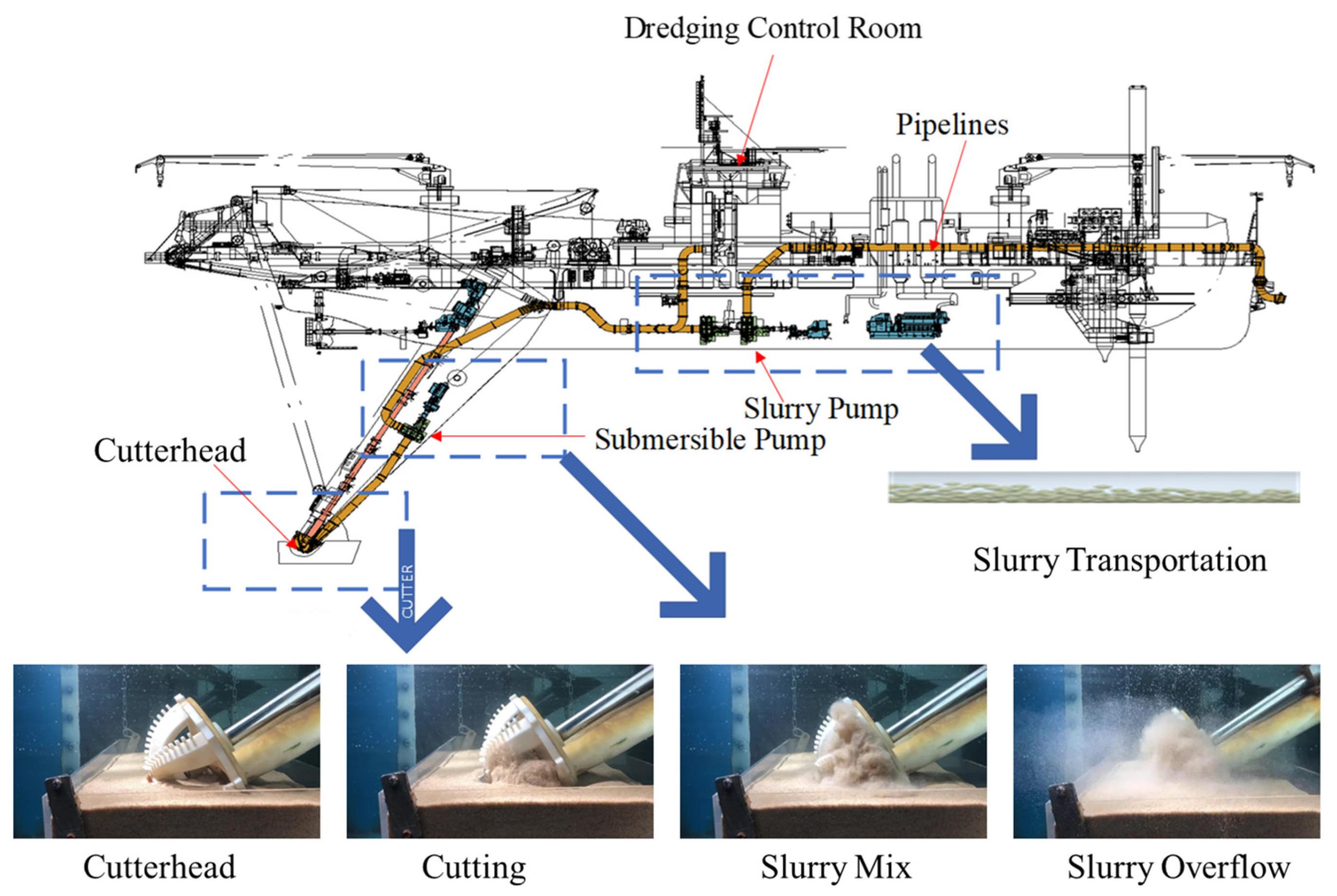
CSDs depend on the suction system to perform the dredging operation. Initially, the cutterhead drive motor rotates the cutterhead, which mixes dredged soil with water to form slurry. The slurry is then sucked into the suction inlet by the slurry pump, which generates the necessary lift to transport the slurry through the pipeline to the designated area. The operation of the suction system can be divided into two stages: the first involves the formation of slurry at the suction inlet, which includes the “contact-breakage-mixing-suction” interaction between the cutterhead and the dredged material; the second stage is the transportation of the slurry. The slurry is drawn into the pipeline at the suction inlet and is pumped through the internal pump, with the lift provided for transport via the slurry pipes (including shore and floating pipes) to the discharge area. The construction process is illustrated in Figure 1, which shows the dredging process of a CSD.

Figure 1.
Construction process diagram of the CSD.
Step 1: Cutterhead Cutting. The cutterhead rotates and cuts the seabed soil, forming a slurry mixture of soil and water. The power of the cutterhead determines the types of soil and rock the dredger can handle.
Step 2: Negative Pressure Suction. As the cutterhead rotates, slurry is formed at the suction inlet. The slurry pump generates negative pressure to draw the slurry from the suction inlet through the suction pipe.
Step 3: Pipeline Transport. The slurry is transported through the dredger’s internal pipeline, with the internal pump providing the necessary lift, and then carried via the on-water/land discharge pipes to the unloading area.
Step 4: Dynamic Regulation. These three steps are interconnected and influence each other. Therefore, the operator in the dredging control room adjusts the cutterhead speed, lateral movement speed, and slurry pump power to balance cutting efficiency and energy consumption, ensuring that the dredger operates under optimal working conditions.
2.2. Dredging Construction Evaluation Parameters
(1) Output
The output is measured by the volume of dredged soil per hour (), calculated as follows:
where volume concentration is the ratio of solid volume to slurry volume, %; is the amount of slurry extracted per hour by the dredger, ; and t denotes time, h.
(2) Cutting Force and Specific Cutting Energy
Cutting force reflects the interaction between the cutterhead and the soil, influenced by parameters such as lateral speed and cutting depth.
Specific cutting energy (energy consumption per unit of material) is an efficiency indicator, directly related to the cutterhead power and the slurry pump’s efficiency.
(3) Slurry Flow Velocity and Concentration
The slurry flow velocity impacts transport efficiency, while slurry concentration determines the volume of soil moved per unit of time. These parameters need to be optimized through calibration experiments.
(4) Post-Dredging Dimension Compliance Rate
The quality parameters, such as the evenness and depth accuracy of the dredged soil layer, must meet the specifications outlined in the dredging contract.
(5) Adaptability Indicators
This includes the dredger’s adaptability to different soil types (such as silt, sand, and clay), its resistance to wind and wave conditions, and its maximum discharge distance.
2.3. Specific Cutting Energy
Specific cutting energy is a key parameter in mechanical processing that measures the energy efficiency of the cutting process. It generally refers to the energy consumed to remove a unit volume of material. Specific cutting energy indicates how efficiently energy is utilized during the cutting process and serves as an important metric for assessing cutting conditions [26,27,28]. For the tool geometry, increasing the rake angle can reduce the cutting force and lower the specific energy, whereas a blunt cutting edge leads to an increase in specific energy. Prolonged cutting can cause tool wear, which increases friction and significantly raises the specific energy. Furthermore, operational parameters also influence changes in specific cutting energy. High-speed cutting may reduce specific energy due to the material softening effect, but excessive speed can lead to faster tool wear. As for feed rate and cutting depth, too small a feed rate can lead to increased specific energy due to the “plowing effect”, while an appropriately increased feed rate improves cutting efficiency. The specific cutting energy is typically calculated using the following formula:
where E represents the energy consumed during the cutting process, J; is the volume of material removed, m3.
For a CSD, the cutter’s specific cutting energy is the ratio of the energy consumed by the cutter to the volume of dredged soil. This value can be used to assess the cutter’s operating condition [29,30]. For example, when cutting through harder materials, the wear on the cutter increases significantly, resulting in a noticeable increase in specific cutting energy. Experienced dredging operators can assess the cutter’s condition and efficiency based on the specific cutting energy, allowing for adjustments to be made to improve performance.
2.4. Effective Specific Cutting Energy
However, this approach is not sufficient for the suction system of a CSD. The traditional definition of specific cutting energy comes from mechanical processing, where the goal is simply to remove metal. In contrast, a CSD not only needs to break the soil and rock but also mix the broken material with water and transport it through a pipeline to a designated location. This process involves breaking the soil and rock, similar to mechanical cutting, but also requires the suction of the broken material into the suction inlet to form slurry. In reality, during the cutting process, the broken soil and rock disperse outward as the cutterhead rotates and are not fully sucked into the suction inlet. Therefore, the energy used to cut this part of the material is considered wasted. Based on this observation, this paper introduces a new model for evaluating energy consumption in the CSD’s cutting system: effective specific cutting energy. This model adjusts the energy consumed by the cutterhead per unit volume of material cut to the energy consumed by the cutterhead to suction per unit volume of dredged soil into the suction inlet.
Since the diameter of the dredger’s slurry transport pipeline is fixed, it is sufficient to know the slurry concentration and flow rate to calculate the volume of slurry being suctioned. The cutterhead is driven by the cutterhead motor, so the power of this motor represents the energy consumption of the cutterhead. A predictive model can be developed to estimate slurry flow rate, slurry concentration, and cutterhead motor power. By utilizing these three key parameters, the effective specific cutting energy of the dredger can be estimated, providing insight into the cutting condition and enabling improvements in cutting efficiency. However, sensor failures are common on dredgers, which can lead to data deviations. To address this, this paper proposes an algorithmic framework that begins with data dimensionality reduction and uses the suction system’s parameters to predict slurry concentration, flow rate, and cutterhead motor power. This algorithm can predict missing data when a sensor fails and substitute these predictions to compute the effective specific cutting energy, thereby assisting operators in improving operational efficiency. Additionally, slurry concentration and flow rate are critical parameters for the automatic control of the suction system. This method contributes to enhancing the automation level of the suction system.
3. Methods and Models
In this section, we propose a feature construction method tailored for the suction system of a CSD, based on the dredger’s cutting mechanism, Spearman correlation coefficient, and PCA dimensionality reduction technique. We then introduce the primary methods used for predicting key parameters.
3.1. Key Theoretical Models of the Dredger
- Suction Inlet Slurry Formation Model
- Soil and Sand Particle Motion Model
This model analyzes the forces acting on soil and sand particles during cutterhead rotation. The motion form is determined based on the relationship between water flow and centrifugal force, and its trajectory is described by the following equation:
where represents the force from water flow, N; is the centrifugal force, N; is the particle shape coefficient; is the cutterhead rotational angular velocity, rad/s; is the cutterhead radius, m; and is the slurry flow velocity, m/s.
- Slurry Pump Models: Clear Water and Slurry Characteristics
The clear water lift formula is as follows:
The slurry lift formula is expressed as follows:
In the clear water lift formula, denotes the clear water lift, kPa, and is the slurry flow velocity, m/s. For the slurry lift formula, represents the slurry lift, kPa; is the slurry specific gravity; is the soil and sand coefficient; is the slurry volume concentration; and is the clear water lift, kPa. This formula is used to assess the effect of slurry on lift.
Total Lift Formula, Including Clear Water and Slurry Characteristics
where is the total clear water lift, kPa; is the water density, kg/m3; is the gravitational acceleration, m/s2; represents the pipeline head loss, m; is the sum of local head losses, m; is the discharge height, m; and is the slurry flow velocity, m/s.
3.2. Feature Engineering
Following the mechanism analysis, we apply the Spearman rank correlation coefficient and Principal Component Analysis (PCA) to reduce the data’s dimensionality, simplifying its complexity for easier processing, analysis, and visualization.
- Spearman Rank Correlation Coefficient
The Spearman rank correlation coefficient, , is used to quantify the strength and direction of a monotonic (nonlinear) relationship between two variables. This coefficient does not require a specific distribution of the variables, making it ideal for handling ordinal data or data with outliers. The formula is as follows:
where is the sample size, and represents the rank differences between the variables and .
- Principal Component Analysis (PCA)
PCA is a widely used unsupervised dimensionality reduction technique that projects high-dimensional data into a lower-dimensional space through linear transformations, while retaining the most significant variance information. The process is as follows:
Step 1: Data Standardization
Given samples, each with variables, the original data matrix is denoted as , where and . To remove the effects of different scales and magnitudes among variables, the data are standardized. The standardized variables are denoted as , and the formula for standardization is as follows:
where is the mean of the j-th variable, and is the standard deviation of the j-th variable.
Step 2: Covariance Matrix Computation
The standardized data matrix is represented as , and its covariance matrix is computed as , where ; .
Step 3: Eigenvalue and Eigenvector Calculation
The covariance matrix S undergoes eigen decomposition, solving the equation to obtain eigenvalues and corresponding eigenvectors , satisfying , , and .
Step 4: Principal Components Determination
The k-th principal component is expressed as follows:
where is the standardized variable.
The contribution rate of the k-th principal component is . This represents the proportion of variance explained by the k-th component. The cumulative contribution rate of the first m components is . When , the first m components are considered sufficient to represent the original data’s information.
3.3. Prediction Algorithms
This paper selects five basic machine learning algorithms: Random Forest (RF) [31,32], eXtreme Gradient Boosting (XGBoost) [33,34], Light Gradient Boosting Machine (LightGBM) [35,36], K-Nearest Neighbor (KNN) [37,38,39], and Gradient Boosting Decision Tree (GBDT) [40,41]. A grid search is performed for each model, focusing on hyperparameters to find the best configuration for each model. These predictions are used as features for the meta-learner (Lasso). The Lasso meta-learner combines all base model predictions, and the final results are generated after training.
3.4. Model Evaluation
The performance of each model is evaluated using four metrics:
(1) Mean Absolute Error (MAE)
MAE measures the average absolute difference between predicted and actual values:
where is the true value, is the predicted value, and is the sample size.
(2) Mean Squared Error (MSE)
MSE quantifies the average squared difference between predicted and actual values:
(3) Root Mean Squared Error (RMSE)
RMSE is the square root of MSE, providing a more intuitive sense of the average error between predicted and true values:
(4) Coefficient of Determination (R2)
R2 measures how well the regression model fits the data and represents the proportion of variance in the dependent variable explained by the model:
where is the mean of the true values.
4. Results and Discussion
4.1. Ship Introduction
The dredger data come from the “Changshi 12” CSD, with working hours from 9:00 a.m. to 3:25 p.m. on 23 June 2018. The data were collected at a frequency of 110 times per minute, totaling over 40,000 data points. The “Changshi 12” is a large CSD equipped with advanced technology and sensors. The vessel is 93 m in length, with a maximum dredging depth of 25 m and a maximum production capacity of 2600 cubic meters per hour. It is equipped with an electric motor-driven underwater pump and two large internal pumps. The dredger is outfitted with more than 200 sensors, with 23 parameters related to the suction system (numbered V0 to V22, with three target variables labeled as target, target1, and target2). These 23 key parameters are shown in the Table 1. For clarity, the parameters are categorized by their location, as follows:

Table 1.
Key parameters of the CSD’s suction system.
Cutterhead Parameters: These parameters have a significant impact on the operation and control of the cutterhead, reflecting its actions and key performance indicators during the dredging process.
Slurry Pump Parameters: These parameters reflect the operational status and key performance indicators of the dredger’s three slurry pumps (one underwater pump and two internal pumps).
Pipeline Parameters: These parameters represent the flow state of slurry within the pipeline.
Environmental Parameters: These reflect the external environment of the cutterhead’s cutting, including the density of water and the soil/rock being cut.
Ship Parameters: These parameters indicate the overall state of the dredger and its production capacity.
4.2. Data Selection and Prediction
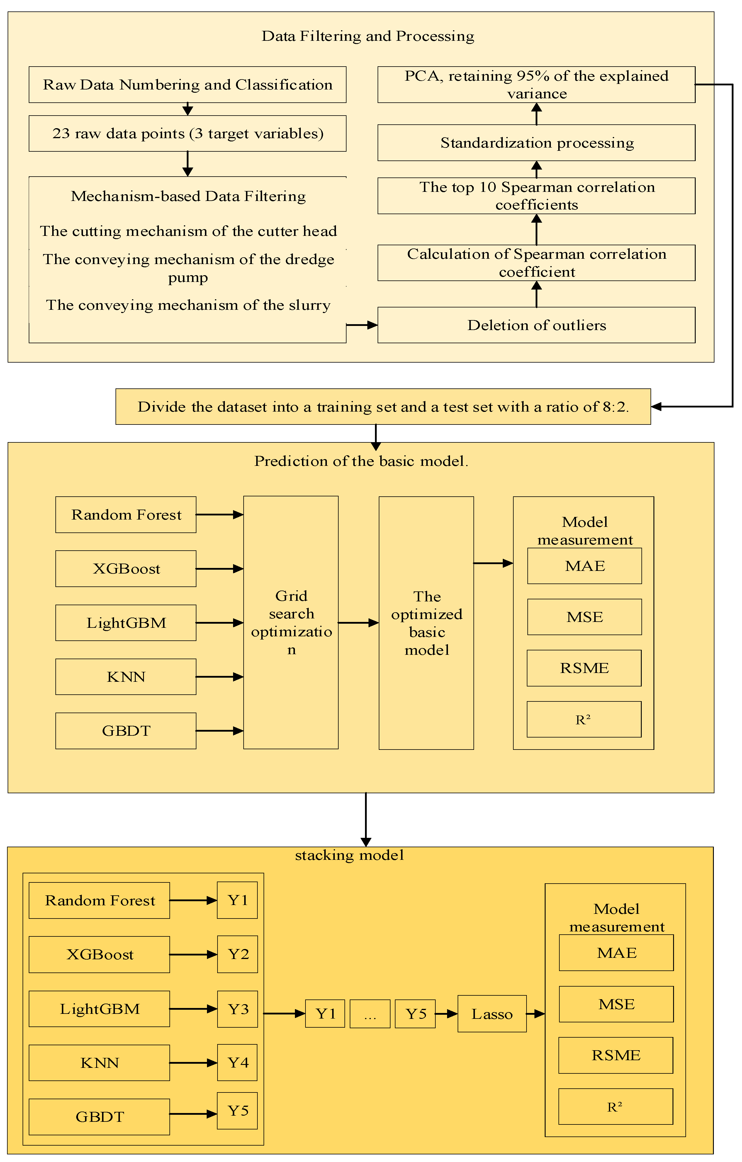
The main operational process of this study is illustrated in Figure 2, the parameter prediction flowchart.
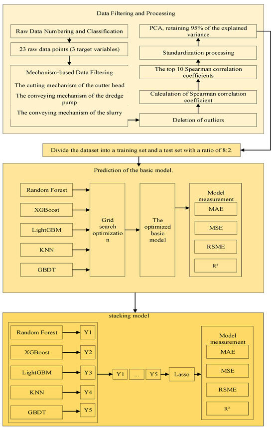
Figure 2.
Parameter prediction flowchart.
The first step involves feature selection based on dredging knowledge and mechanics. During the dredging process, parameters V20 and V21 are constants. These data are derived from environmental measurements in the area prior to the dredging operation, so these two parameters can be removed. Additionally, as indicated by Formula (3), parameter V19 is calculated from parameters V20, V21, and V12. Since V12 is a target variable in this study, V19 is also removed.
where represents the slurry concentration, %; is the instantaneous flow, m3; is the slurry velocity, and pipeline diameter is a constant value, m.
Since slurry flow velocity is one of our target variables, parameters V22 (instantaneous production rate) and V18 (flow rate) are removed. Additionally, it was observed that the speed of the No. 2 internal pump remained at 0, indicating that the No. 2 internal pump was not in operation, and the slurry lift came entirely from the No. 1 internal pump and the underwater pump. Based on Formulas (5)–(7), parameters V16 and V17 are also removed.
Following the mechanistic analysis, the original dataset, which initially had 23 variables, was reduced to a target dataset containing only 16 variables. Outliers are then removed based on the data’s characteristics. First, states where V22 is less than or equal to 0 are observed, as the instantaneous production rate cannot be negative. A value of 0 indicates that the dredger was not working, so these data points are deleted. Secondly, the three target variables (slurry concentration, cutterhead power, and slurry flow velocity) cannot be less than or equal to 0 during the dredging process, so this data is also deleted. Finally, any remaining missing values are checked and removed to complete the outlier processing.
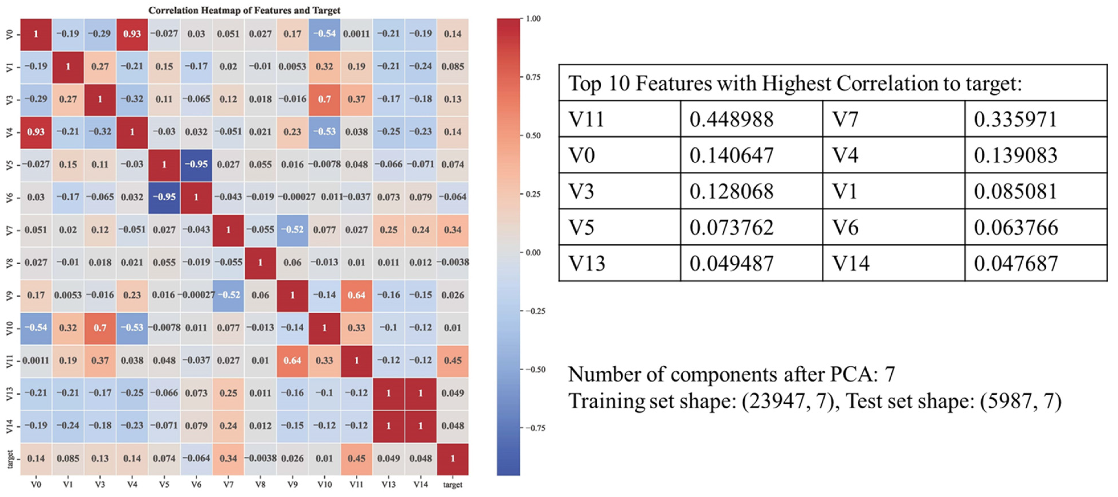
After excluding target, target1, and target2, the correlation coefficient matrix between the remaining 13 features and target, target1, and target2 is calculated. The result is shown in the figure, and the top 10 features with the highest correlation coefficients are selected. PCA dimensionality reduction is performed on these 10 features, with a cumulative contribution rate set, and the number of features is retained at this point. The data are divided into training and test sets with an 80:20 ratio. After data cleaning, the dataset contains 23,947 sets of training data and 5987 sets of test data. The processing results are shown in Figure 3, Figure 4 and Figure 5.
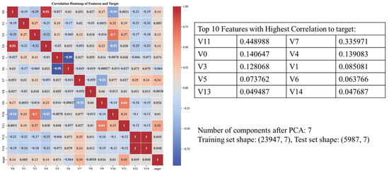
Figure 3.
Correlation coefficient diagram of target and the dimensions of the training set and the test set after PCA processing.
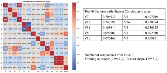
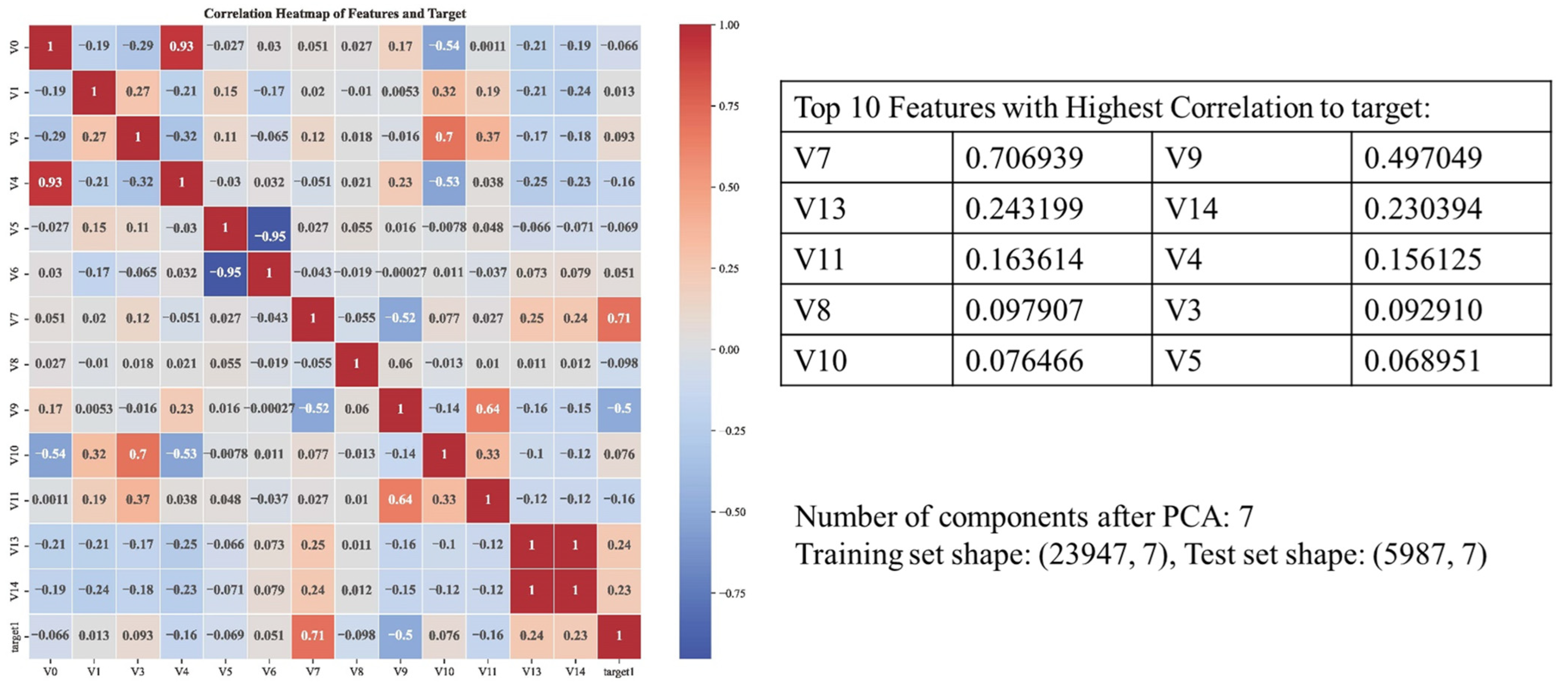
Figure 4.
Correlation coefficient diagram of target1 and the dimensions of the training set and the test set after PCA processing.
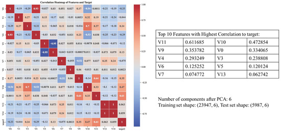
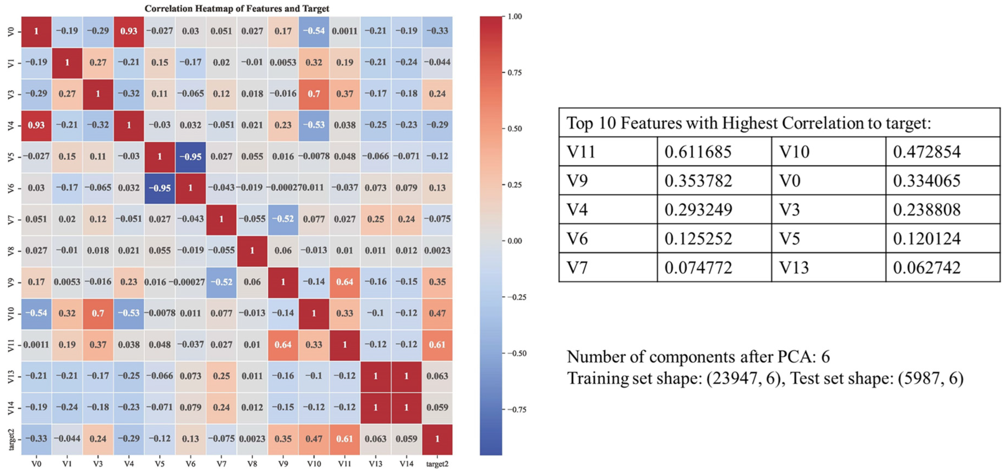
Figure 5.
Correlation coefficient diagram of target2 and the dimensions of the training set and the test set after PCA processing.
As can be seen, the correlation between target, target1, and target2 with the remaining features was calculated, and the top 10 features with the highest correlations were selected. These features include the following:
V0—Angle of the cutter ladder;
V3—Rotation speed of the cutter;
V4—Depth of the dredging;
V5—Left horizontal movement speed;
V7—Vacuum;
V11—Discharge pressure of the No. 1 slurry pump;
V13—Trolley trip.
These parameters are highly correlated with all three target variables. However, when applying PCA and retaining variables that account for at least 95% of the cumulative contribution rate, both target and target1 retained seven features, while target2 only required six features. A grid search was used to determine the optimal hyperparameters for RF, XGBoost, LightGBM, KNN, and GBDT. These optimized models were used as base models, and their prediction results were then input into a meta-learner (Lasso). By employing Lasso as the meta-learner to combine the predictions from all the base models, the final prediction results were generated after training.
The results of the program are shown in Table 2, Table 3 and Table 4, which display the best hyperparameters optimized through grid search for RF, XGBoost, LightGBM, KNN, and GBDT, along with the prediction results for slurry concentration, cutterhead motor power, and slurry flow velocity. MAE, MSE, RMSE, and R2 were used as evaluation metrics to assess the prediction performance. Additionally, comparison curves of predicted versus actual values for slurry concentration, cutterhead motor power, and slurry flow velocity under different models are shown in Figure 6, Figure 7 and Figure 8.
Table 2.
Prediction results of the slurry concentration (target).
Table 3.
Prediction results of the cutterhead motor power (target1).
Table 4.
Prediction results of the slurry flow velocity (target2).
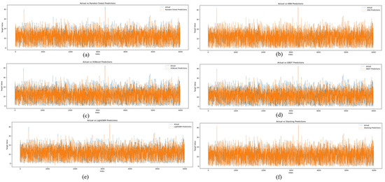
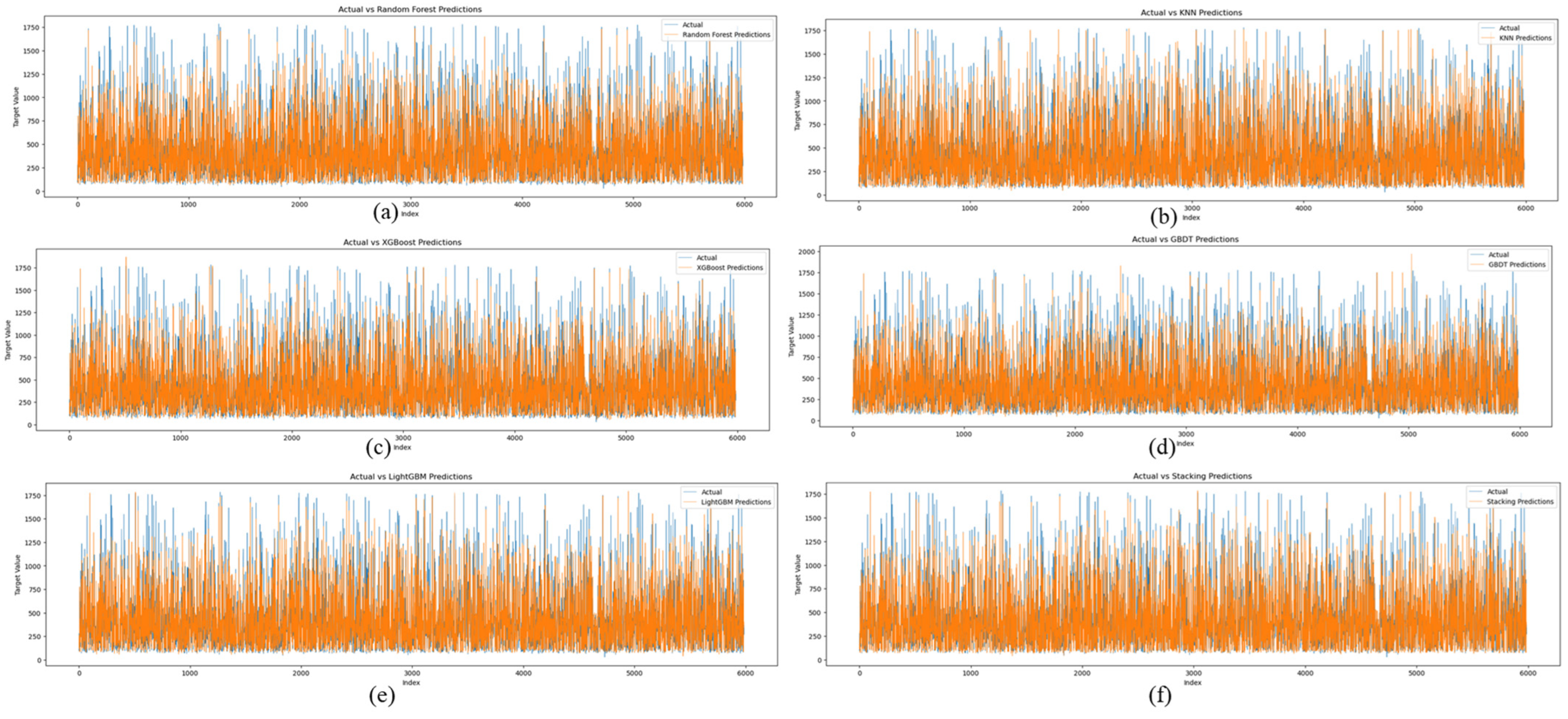
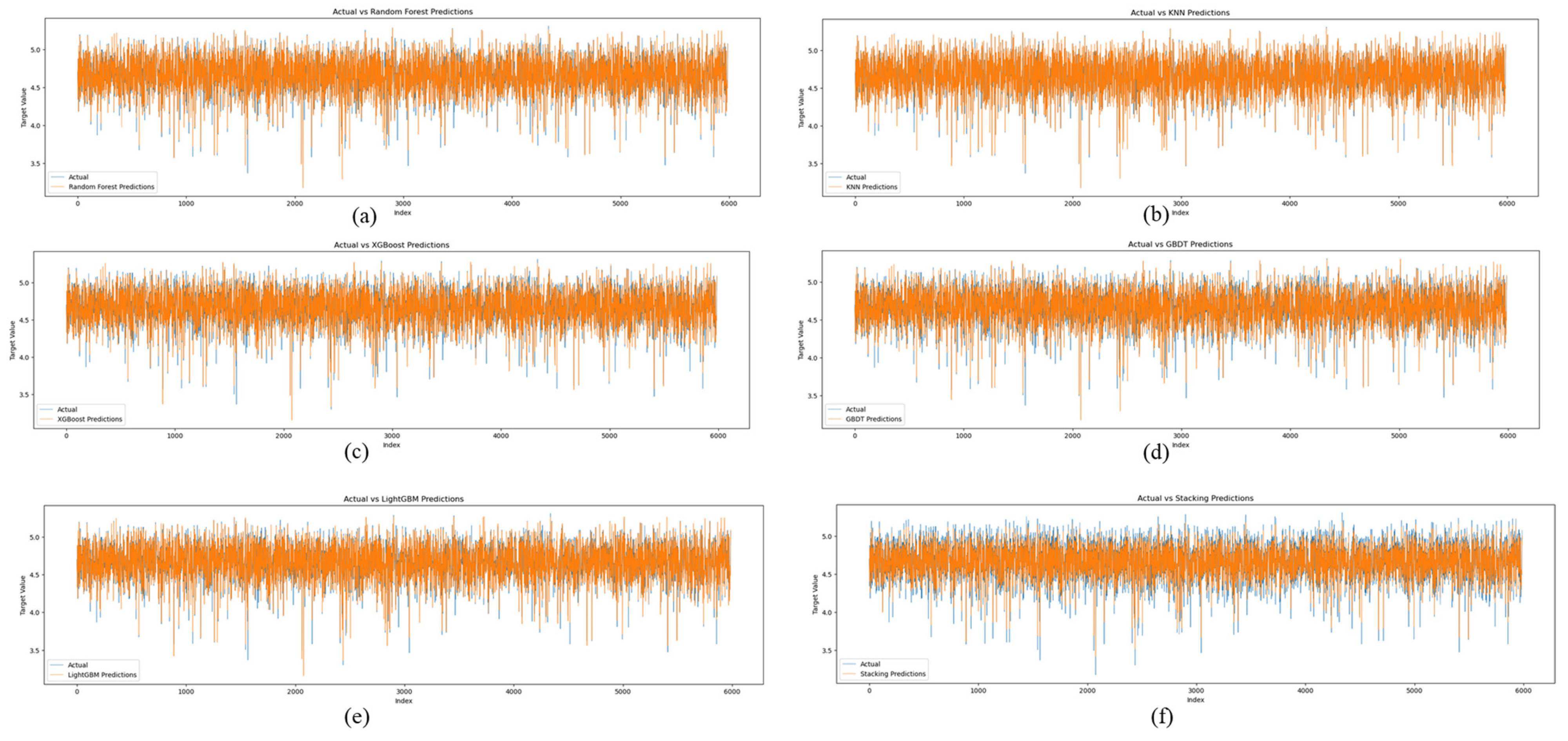
Figure 6.
Comparison diagram of the slurry concentration—model prediction results and actual values: (a) RF, (b) KNN, (c) XGBoost, (d) GBDT, (e) LightGBM, and (f) Stacking models.
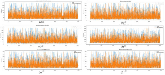
Figure 7.
Comparison of the cutterhead motor power—model prediction results and actual values: (a) RF, (b) KNN, (c) XGBoost, (d) GBDT, (e) LightGBM, and (f) Stacking models.

Figure 8.
Comparison of the slurry flow velocity—model prediction results and actual values: (a) RF, (b) KNN, (c) XGBoost, (d) GBDT, (e) LightGBM, and (f) Stacking models.
For the prediction results of slurry concentration, six models, namely RF, Extreme XGBoost, LightGBM, KNN, GBDT, and Stacking models, were used to predict the slurry concentration. Taking MAE, MSE, RMSE, and R2 as evaluation metrics, the results show that all models have good prediction effects, with R2 values all above 93%. Among them, the R2 value of KNN is the highest, reaching 0.9931; the R2 of the Stacking Model is 0.9906; and the R2 of Random Forest is 0.9782. In terms of MAE, KNN has the lowest value of 0.1862; for MSE, KNN is 0.2832; and in the RMSE value, KNN is 0.5322. For the prediction results of cutterhead motor power, the prediction accuracy of the abovementioned six models for cutterhead motor power is lower than that for slurry concentration. The R2 values are in the range of 83–86%. Specifically, the R2 of Random Forest is 0.8633, the R2 of the Stacking model is 0.8618, and the R2 value of LightGBM is 0.8605. In terms of MAE value, Random Forest is 74.0720; for MSE, Random Forest is 16,144.1292; and in terms of RMSE, Random Forest is 127.0595. For the prediction results of slurry flow velocity, the R2 values of the six models for predicting slurry flow velocity are also all above 93%. The R2 value of KNN is 0.9847, the R2 of the Stacking Model is 0.9539, and the R2 of Random Forest is 0.9696. In terms of MAE, KNN has the lowest value of 0.0102; for MSE, KNN is 0.0010; and for the RMSE value, KNN is 0.0309. In comprehensive comparison, overall, the Random Forest and Stacking model show relatively better accuracy in predicting the three parameters of slurry concentration, cutterhead motor power, and slurry flow velocity.
A comparative analysis of the prediction accuracy of the model proposed in this paper and the models in other studies was conducted (see Table 5 for details). The results show that different models have their own advantages and disadvantages when predicting power, slurry concentration, and flow velocity.
Table 5.
Comparison of prediction accuracy.
For the prediction of flow velocity, the R2 value of the KNN model in this paper is 0.9847; the R2 value of the Pearson model in other papers is 0.9935. In terms of slurry concentration prediction, the R2 value of the KNN model in this paper is 0.9931; the R2 value of the proposed PCA-LSTM model in other papers is as high as 0.9999. The existence of a small error may be due to the fact that the data volumes of the datasets at hand are different, resulting in different selections of eigenvalues and causing prediction errors of the models. In terms of power prediction, the R2 value of the RF model used in this paper is 0.8633; the R2 value of the CNN-LSTM Encode-Decode model adopted in other papers reaches 0.9632. This indicates that in the prediction of this indicator, the CNN-LSTM Encode-Decode model performs better, and its prediction accuracy is significantly higher than that of the RF model. It may benefit from the effective capture and in-depth mining of the time series characteristics of the data, so as to more accurately predict the power changes. Although the accuracy of the model proposed in this paper in predicting some parameters is slightly inferior to that of the models in other studies, it still has a certain degree of reliability and effectiveness as a whole and can provide valuable references for the prediction of relevant parameters of cutter suction dredgers. Future research can further optimize the model to improve its accuracy and stability in predicting various parameters.
In actual dredging operations, cutterhead motor power is calculated from the cutterhead motor current and voltage, which are known to have high accuracy and sensor reliability. Among the sensors, the cutterhead motor power sensor has the highest accuracy and reliability, while the slurry concentration sensor has the lowest accuracy and reliability. During dredging operations, when all these sensors fail, the need to simultaneously predict all three parameters to compute the effective specific cutting energy is quite rare. Compared to the other models used in this study, the RF and Stacking models demonstrate good accuracy in predicting these parameters.
5. Conclusions
The actual dredging process is highly integrated, particularly in the coordination between the cutterhead and the underwater pump. For example, cutting speed generally refers to the traverse swing speed of the dredger, and there exists an optimal cutting speed that minimizes specific cutting energy while maximizing cutting volume. However, when the concentration at the cutterhead becomes too high, it can block the cutter, leading to operational inefficiencies. An excessive concentration also causes the mud flow velocity to drop below the critical threshold, resulting in sediment clogging the pipeline. Additionally, material properties significantly influence the cutting process. Harder rocks typically require more specific cutting energy, which exacerbates wear on the cutter teeth, further increasing energy consumption. Therefore, dynamic adjustment of parameters such as cutter rotational speed and traverse speed is essential to prevent damage to the cutterhead. In practice, multiple factors interact and affect the final construction result. These parameters are displayed and summarized on the dredging console, but it is challenging to account for all of them during operations. This is why the concept of effective specific cutting energy, which integrates both cutting and suction processes, is introduced. This key parameter assists construction workers in evaluating the dredging operation’s status.
For the Cutter Suction Dredger (CSD) cutting system, the effective specific cutting energy reflects the interaction between the cutterhead system and the pump-pipeline system. This metric is crucial for improving construction efficiency. In this study, we introduced effective specific cutting energy as a new indicator for assessing the operational efficiency of CSDs. A calculation method was developed, enabling the determination of effective specific cutting energy based on cutterhead motor power, slurry concentration, and slurry flow velocity. Additionally, we created a machine learning framework to predict specific cutting energy using suction system parameters. The feasibility of this approach was validated with real ship data from the “Changshi 12” CSD.
The RF and Stacking models demonstrated excellent prediction accuracy for the three key parameters: slurry concentration, cutter motor power, and slurry flow velocity. Taking the prediction of slurry concentration as an example, the R2 value of the RF model was 0.9782, and that of the Stacking model was 0.9906. In terms of the prediction of cutterhead motor power, the R2 value of the RF model was 0.8633, and that of the Stacking model was 0.8618. For the prediction of slurry flow velocity, the R2 value of the RF model was 0.9696, and that of the Stacking model was 0.9539. By integrating dredger-specific knowledge and experience in data feature selection and outlier removal, this method significantly reduced data dimensionality. The Spearman correlation analysis revealed that parameters such as the angle of the cutter ladder, rotation speed of the cutter, dredging depth, left horizontal movement speed, vacuum, discharge pressure of the No. 1 slurry pump, and trolley trip all have a high correlation with slurry concentration, cutterhead motor power, and slurry flow velocity.
However, dredgers operate in a variety of modes, such as using only the underwater pump, using both the underwater pump and No. 1/No. 2 pump, or using all pumps simultaneously. Each operational mode involves different parameters, and this study addressed only one operational mode with a limited set of operational parameters. The effects of other operational modes and parameters will require further investigation in future studies.
Author Contributions
Conceptualization, J.Y.; methodology, J.Y. and S.F.; software, J.Y.; validation, J.Y.; formal analysis, J.Y., T.X. and H.X.; data curation, K.Y., J.Y. and T.Y.; writing—original draft preparation, J.Y.; writing—review and editing, K.Y., S.F. and J.Y.; visualization, J.Y.; supervision, S.F.; funding acquisition, S.F. All authors have read and agreed to the published version of the manuscript.
Funding
This research was funded by National Natural Science Foundation of China under Grant No. 52071240.
Data Availability Statement
Data is available when required.
Conflicts of Interest
The authors declare no conflicts of interest. The funders had no role in the design of the study; in the collection, analyses, or interpretation of data; in the writing of the manuscript; or in the decision to publish the results.
Abbreviations
The following abbreviations are used in this manuscript:
| CSD | Cutter Suction Dredger |
| PCA | Principal Component Analysis |
| RF | Random Forest |
| KNN | K-Nearest Neighbor |
| XGBoost | eXtreme Gradient Boosting |
| GBDT | Gradient Boosting Decision Tree |
| LightGBM | Light Gradient Boosting Machine |
| MAE | Mean Absolute Error |
| MSE | Mean Squared Error |
| RSME | Root Mean Squared Error |
| R2 | Coefficient of Determination |
References
- Ouyang, Y.P.; Yang, Q.; Chen, X.Q.; Xu, Y.F. An Analytical Model for Rock Cutting with a Chisel Pick of the Cutter Suction Dredger. J. Mar. Sci. Eng. 2020, 8, 806. [Google Scholar] [CrossRef]
- Reddy, N.V.K.; Pothal, J.K.; Barik, R.; Senapati, P.K. Pipeline Slurry Transportation System: An Overview. J. Pipel. Syst. Eng. Pract. 2023, 14, 15. [Google Scholar] [CrossRef]
- Miedema, S.A. A head loss model for slurry transport in the heterogeneous regime. Ocean Eng. 2015, 106, 360–370. [Google Scholar] [CrossRef]
- Miedema, S.A. An overview of theories describing head losses in slurry transport a tribute to some of the early researchers. In Proceedings of the 32nd ASME International Conference on Ocean, Offshore and Arctic Engineering, Nantes, France, 9–14 June 2013. [Google Scholar]
- Bai, S.; Li, M.C.; Kong, R.; Han, S.; Li, H.; Qin, L. Data mining approach to construction productivity prediction for cutter suction dredgers. Autom. Constr. 2019, 105, 13. [Google Scholar] [CrossRef]
- Yue, P.; Zhong, D.H.; Miao, Z.J.; Yu, J. Prediction of Dredging Productivity Using a Rock and Soil Classification Model. J. Waterw. Port Coast. Ocean Eng. 2015, 141, 7. [Google Scholar] [CrossRef]
- Li, J.Y.; Shi, Y.Y.; Rao, K.P.; Zhao, K.Y.; Xiao, J.F.; Xiong, T.; Huang, Y.Z.; Huang, Q.B. The Design and Analysis of Double Cutter Device for Hinge and Suction Dredger Based on Feedback Control Method. Appl. Sci. 2022, 12, 3793. [Google Scholar] [CrossRef]
- Fu, J.K.; Tian, H.J.; Song, L.G.; Li, M.C.; Bai, S.; Ren, Q.B. Productivity estimation of cutter suction dredger operation through data mining and learning from real-time big data. Eng. Constr. Archit. Manag. 2021, 28, 2023–2041. [Google Scholar] [CrossRef]
- Tang, H.Z.; Wang, Q.F.; Bi, Z.Y. Expert system for operation optimization and control of cutter suction dredger. Expert Syst. Appl. 2008, 34, 2180–2192. [Google Scholar] [CrossRef]
- Tang, J.Z.; Wang, Q.F.; Zhong, T.Y. Automatic monitoring and control of cutter suction dredger. Autom. Constr. 2009, 18, 194–203. [Google Scholar] [CrossRef]
- Wei, C.Y.; Ni, F.S.; Chen, X.J. Obtaining Human Experience for Intelligent Dredger Control: A Reinforcement Learning Approach. Appl. Sci. 2019, 9, 1769. [Google Scholar] [CrossRef]
- Wei, C.Y.; Wei, Y.; Ji, Z. Model predictive control for slurry pipeline transportation of a cutter suction dredger. Ocean Eng. 2021, 227, 11. [Google Scholar] [CrossRef]
- Wei, C.Y.; Wang, H.; Bai, H.A.; Ji, Z.; Liu, Z.H. PPLC: Data-driven offline learning approach for excavating control of cutter suction dredgers. Eng. Appl. Artif. Intell. 2023, 125, 13. [Google Scholar] [CrossRef]
- Li, M.C.; Kong, R.; Han, S.; Tian, G.P.; Qin, L. Novel Method of Construction-Efficiency Evaluation of Cutter Suction Dredger Based on Real-Time Monitoring Data. J. Waterw. Port Coast. Ocean Eng. 2018, 144, 14. [Google Scholar] [CrossRef]
- Wang, B.; Fan, S.D.; Jiang, P.; Chen, Y.; Zhu, H.H.; Xiong, T. Cutting state estimation and time series prediction using deep learning for Cutter Suction Dredger. Appl. Ocean Res. 2023, 134, 9. [Google Scholar] [CrossRef]
- Yang, K.; Yuan, J.L.; Xiong, T.; Wang, B.; Fan, S.D. A Novel Principal Component Analysis Integrating Long Short-Term Memory Network and Its Application in Productivity Prediction of Cutter Suction Dredgers. Appl. Sci. 2021, 11, 8159. [Google Scholar] [CrossRef]
- Wang, B.; Fan, S.D.; Chen, Y.; Zheng, L.Y.; Zhu, H.H.; Fang, Z.L.; Zhang, M. The replacement of dysfunctional sensors based on the digital twin method during the cutter suction dredger construction process. Measurement 2022, 189, 14. [Google Scholar] [CrossRef]
- Wang, B.; Zio, E.; Fan, S.D. Reliability evaluation of the hybrid-redundancy sensor fault tolerate system in the dredging perception system. Ocean Eng. 2023, 281, 16. [Google Scholar] [CrossRef]
- Han, S.; Li, H.; Li, M.C.; Tian, H.J.; Qin, L.; Yu, Y.; Ma, J. Intelligent short-term forecasting for mud concentration in CSD dredging construction. Ocean Eng. 2022, 266, 17. [Google Scholar] [CrossRef]
- Chen, Y.; Ren, Q.B.; Li, M.C.; Tian, H.J.; Qin, L.; Wu, D.C. Prediction of submarine soil dredging difficulty scale in cutter suction dredger construction with clustering-based deep learning. Eng. Appl. Artif. Intell. 2025, 147, 110370. [Google Scholar] [CrossRef]
- Cheng, T.; Lu, Q.R.; Kang, H.R.; Fan, Z.Y.; Bai, S. Productivity Prediction and Analysis Method of Large Trailing Suction Hopper Dredger Based on Construction Big Data. Buildings 2022, 12, 1505. [Google Scholar] [CrossRef]
- Jiang, P.; Yang, Y.K.; Cao, C.H.; Dong, X.Y. Implementation of Constant Power Control for a Reamer Using a Fuzzy PID Algorithm. Mathematics 2025, 13, 647. [Google Scholar] [CrossRef]
- Wang, W.; Shen, Y.C.; Wang, L.Y.; Wang, D.S.; Bai, Y.M. Design of Dredging Process Control System for Cutter Suction Dredger. In Proceedings of the 33rd Chinese Control and Decision Conference (CCDC), Kunming, China, 22–24 May 2021; pp. 5932–5937. [Google Scholar]
- Xin, C.H.; Yue, S.H.; Yang, L. Feedback Control System in Dredging Engineering Based on Convolutional Neural Network Prediction. In Proceedings of the 2021 IEEE International Instrumentation and Measurement Technology Conference (I2MTC), Glasgow, UK, 17–20 May 2021. [Google Scholar]
- Zhou, B.L.; Yu, M.H.; Guo, J. Hybrid optimization algorithm for estimating soil parameters of spoil hopper deposition model for trailing suction hopper dredgers. J. Intell. Fuzzy Syst. 2024, 46, 1813–1831. [Google Scholar] [CrossRef]
- Balogun, V.A.; Edem, I.F.; Adekunle, A.A.; Mativenga, P.T. Specific energy based evaluation of machining efficiency. J. Clean Prod. 2016, 116, 187–197. [Google Scholar] [CrossRef]
- Cho, J.W.; Jeon, S.; Jeong, H.Y.; Chang, S.H. Evaluation of cutting efficiency during TBM disc cutter excavation within a Korean granitic rock using linear-cutting-machine testing and photogrammetric measurement. Tunn. Undergr. Space Technol. 2013, 35, 37–54. [Google Scholar] [CrossRef]
- He, X.Q.; Xu, C.S. Specific Energy as an Index to Identify the Critical Failure Mode Transition Depth in Rock Cutting. Rock Mech. Rock Eng. 2016, 49, 1461–1478. [Google Scholar] [CrossRef]
- Nieuwboer, B.J.; van Rhee, C.; Keetels, G.H. Towards simulating flow induced spillage in dredge cutter heads using DEM-FVM. Ocean Eng. 2023, 275, 13. [Google Scholar] [CrossRef]
- Mahgoub, M.; Keetels, G.H.; Alhaddad, S. Impact of operational parameters on turbidity generation in cutter suction dredging: Insights from a numerical model and sensitivity analysis. Appl. Ocean Res. 2025, 154, 104312. [Google Scholar] [CrossRef]
- Belgiu, M.; Dragut, L. Random forest in remote sensing: A review of applications and future directions. ISPRS J. Photogramm. Remote Sens. 2016, 114, 24–31. [Google Scholar] [CrossRef]
- Breiman, L. Random forests. Mach. Learn. 2001, 45, 5–32. [Google Scholar] [CrossRef]
- Chen, M.H.; Liu, Q.Y.; Chen, S.H.; Liu, Y.C.; Zhang, C.H.; Liu, R.H. XGBoost-Based Algorithm Interpretation and Application on Post-Fault Transient Stability Status Prediction of Power System. IEEE Access 2019, 7, 13149–13158. [Google Scholar] [CrossRef]
- Chen, T.Q.; Guestrin, C.; Assoc Comp, M. XGBoost: A Scalable Tree Boosting System. In Proceedings of the 22nd ACM SIGKDD International Conference on Knowledge Discovery and Data Mining (KDD), San Francisco, CA, USA, 13–17 August 2016; pp. 785–794. [Google Scholar]
- Ke, G.L.; Meng, Q.; Finley, T.; Wang, T.F.; Chen, W.; Ma, W.D.; Ye, Q.W.; Liu, T.Y. LightGBM: A Highly Efficient Gradient Boosting Decision Tree. In Proceedings of the 31st Annual Conference on Neural Information Processing Systems (NIPS), Long Beach, CA, USA, 4–9 December 2017. [Google Scholar]
- Ma, X.J.; Sha, J.L.; Wang, D.H.; Yu, Y.B.; Yang, Q.; Niu, X.Q. Study on a prediction of P2P network loan default based on the machine learning LightGBM and XGboost algorithms according to different high dimensional data cleaning. Electron. Commer. Res. Appl. 2018, 31, 24–39. [Google Scholar] [CrossRef]
- Weinberger, K.Q.; Saul, L.K. Distance Metric Learning for Large Margin Nearest Neighbor Classification. J. Mach. Learn. Res. 2009, 10, 207–244. [Google Scholar]
- Wu, X.D.; Kumar, V.; Quinlan, J.R.; Ghosh, J.; Yang, Q.; Motoda, H.; McLachlan, G.J.; Ng, A.; Liu, B.; Yu, P.S.; et al. Top 10 algorithms in data mining. Knowl. Inf. Syst. 2008, 14, 1–37. [Google Scholar] [CrossRef]
- Zhang, M.L.; Zhou, Z.H. ML-KNN: A lazy learning approach to multi-label leaming. Pattern Recognit. 2007, 40, 2038–2048. [Google Scholar] [CrossRef]
- Friedman, J.H. Greedy function approximation: A gradient boosting machine. Ann. Stat. 2001, 29, 1189–1232. [Google Scholar] [CrossRef]
- Natekin, A.; Knoll, A. Gradient boosting machines, a tutorial. Front. Neurorobotics 2013, 7, 21. [Google Scholar] [CrossRef]

Disclaimer/Publisher’s Note: The statements, opinions and data contained in all publications are solely those of the individual author(s) and contributor(s) and not of MDPI and/or the editor(s). MDPI and/or the editor(s) disclaim responsibility for any injury to people or property resulting from any ideas, methods, instructions or products referred to in the content. |
© 2025 by the authors. Licensee MDPI, Basel, Switzerland. This article is an open access article distributed under the terms and conditions of the Creative Commons Attribution (CC BY) license (https://creativecommons.org/licenses/by/4.0/).