Abstract
This study proposes a control method for Remotely Operated Vehicles (ROVs) to actively dock with AUVs, to address the limitations of traditional docking and recovery schemes for Autonomous Underwater Vehicles (AUVs), such as restricted maneuverability and external disturbances. Firstly, a process and control strategy for ROV active docking with AUVs is designed, improving docking safety. Secondly, a Nonlinear Model Predictive Controller (NMPC) based on a Gaussian Function Sliding Mode Observer (GFSMO) compensation is designed for the ROV, generating smooth control inputs to achieve high-precision trajectory tracking and real-time docking. Finally, a joint simulation experiment is established through WEBOTS 2023a and MATLAB 2023a, verifying the superiority and feasibility of the designed controller and the proposed method. After parameter optimization, the simulation results show the method proposed in this study has a 90% success rate in 10 docking experiments under different disturbances.
1. Introduction
As an essential tool for marine resource exploration, the demand for Autonomous Underwater Vehicles (AUVs) [1,2] has been steadily increasing. However, the endurance and real-time communication capabilities of AUVs are limited by battery capacity and underwater environmental conditions, necessitating periodic recovery for tasks such as data transmission, equipment maintenance, and battery replacement [3,4]. With the continuous development of operational requirements and technological advancements, various underwater docking and recovery methods for AUVs have emerged. By adopting underwater docking and recovery, tasks such as energy replenishment, command configuration, and data exchange can be carried out while underwater. This capability allows AUVs to quickly resume operations without the need to return to the deck. However, underwater AUV docking and recovery technologies are affected by factors such as the maneuverability of AUVs, the size of the docking device, and external current disturbances, which increase the risk of docking [5]. Therefore, achieving safe and reliable underwater docking and recovery of AUVs has become a critical question in underwater operations.
Most AUV docking and recovery methods can be classified into two categories: fixed docking stations and mobile docking stations. Fixed docking stations are typically deployed on the seabed or in a floating state, with pre-programmed homing trajectories for autonomous docking [6,7,8]. This method simplifies the target positioning process, but limits the operational range of the AUV. In contrast, mobile docking stations rely on ships or floating carriers for positioning, and AUVs autonomously identify and dock with the station using sensors [9,10,11]. This method expands the operational range of AUVs, but poses challenges for their autonomous positioning capabilities. Both approaches require AUVs to have strong maneuverability and increase the cost of recovery. To address these issues, researchers have proposed using Remotely Operated Vehicles (ROVs) [12,13] to actively dock with AUVs [14,15,16], thus reducing the control requirements for AUVs and improving the docking and recovery efficiency. However, current active docking strategies for AUVs using ROVs primarily rely on remote operation. Remote operation of ROVs for AUV docking requires operator training, which limits the universality of the system [15]. Furthermore, constrained by signal transmission delays, operator responses may lack timeliness, thus increasing collision risks during docking [17].
To overcome these challenges, developing an autonomous ROV active docking control method for AUVs is an urgent problem. Its implementation will help reduce docking and recovery costs and improve efficiency. In this process, the ROV must achieve precise tracking and positioning of the target. Researchers have conducted related studies on ROV underwater docking and tracking control. Trslic et al. [17] developed a seabed-resident ROV docking station, applying an advanced visual navigation system to the ROV and using a PID algorithm to achieve precise docking between the ROV and the docking station. However, in close-range docking, the performance of the PID control deteriorates due to sensor noise. Li et al. [18] developed a learning-based particle swarm optimization fuzzy rule controller based on region-based fully convolutional networks for visual positioning, achieving target capture without considering the ROV’s horizontal speed and position information, but the complexity of the controller design increased significantly. However, high-precision ROV tracking control has garnered widespread attention from scholars. Mu et al. [19] developed a double-loop sliding mode controller with an ocean current observer for ROV trajectory tracking, reducing the overshoot error by and the response time from 16.3 s to 0.07 s compared to traditional sliding mode control. However, the chattering issue of sliding mode control cannot be ignored.
Nonlinear Model Predictive Control (NMPC) has attracted significant attention due to its strong robustness in handling nonlinear and multi-constraint problems, as demonstrated in terrestrial robot tracking control. In the context of AUV autonomous docking, Uchihori et al. [20] proposed a linear parameter-varying model predictive control (LPV-MPC) method for AUV underwater docking, simplifying the AUV’s nonlinear model into an LPV model combined with a thruster allocation algorithm to reduce computational pressure and achieve high-precision docking under current disturbances. Wu et al. [21] designed an Adaptive Integral Event-Triggered Nonlinear Model Predictive Control (AIET-NMPC) for AUV tracking with a mobile docking station, dynamically adjusting the trigger threshold and introducing exponential robust constraints to enhance system stability and achieve safe docking. In trajectory optimization, Zheng et al. [22] proposed a coordinated trajectory tracking method for Underwater Vehicle Manipulator Systems (UVMSs) using model predictive control, optimizing system steering performance by actively utilizing the drag force generated by the manipulator. For ROV tracking control, Anderlini et al. [23] proposed an Adaptive Model Predictive Control (AMPC) for ROVs carrying objects, optimizing control actions and suppressing excessive control variations compared to sliding mode and PID control. However, due to system nonlinearities and online system identification, the tracking error of the ROV increased, reducing its performance. Overall, while NMPC has advantages in autonomous ROV docking tasks, the uncertainty of the model remains a significant challenge for control systems.
To address these issues, this paper proposes a Gaussian Function Sliding Mode Observer (GFSMO)-compensated Nonlinear Model Predictive Controller (GFSMO-NMPC) for autonomous ROV active docking with AUVs. The controller consists of two parts. The first part is GFSMO, which effectively solves the overshoot and lag issues caused by initial errors while ensuring the transient response of the sliding mode observer, used to estimate ROV model uncertainties and external disturbances. The second part is NMPC, which performs rolling optimization based on the desired state, ROV state information, and constraints to derive the optimal control sequence, achieving precise trajectory tracking and stable docking with the AUV. The main contributions of this study are as follows:
- The process and control strategy for ROV active docking with AUVs is designed, improving docking safety.
- A GFSMO-NMPC controller is proposed to enhance system control performance.
- A joint simulation experiment is established through WEBOTS and MATLAB, verifying the superiority and feasibility of the designed controller and the proposed method.
This paper is structured as follows: Section 2 describes the ROV active docking process and the control strategy. Section 3 establishes the ROV dynamic model. Section 4 designs the GFSMO-NMPC controller for the docking control strategy. Simulation results are provided in Section 5 to validate the proposed method and the docking control strategy. Section 6 introduces the “Experimental guides”. Section 7 concludes the paper.
2. Docking Process and Control Strategy
This paper assumes that the ROV possesses reliable autonomous localization and target AUV localization capabilities in real-world scenarios. The ROV active docking process is systematically divided into three stages: long-distance approach, relative hovering, and contact docking. Transitions between these stages are governed by the Euclidean distance d between the ROV and AUV, as illustrated in Figure 1. To ensure docking safety, two critical constraints are defined based on engineering experience and practical project requirements:
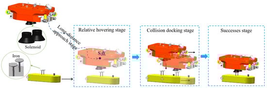
Figure 1.
ROV active docking AUV scheme.
- Hovering offset point S: A safety offset point S is established 2 m above the AUV’s docking interface. This offset prevents potential collisions caused by ROV over-approximation during the approach stage. The 2 m distance is empirically determined to balance vertical collision avoidance and the effective detection range of the binocular camera.
- Steady-state circle diameter D: Maintaining absolute horizontal stationarity relative to a moving AUV is challenging due to hydrodynamic interactions. Therefore, a horizontal “steady-state circle” with a diameter D = 10 cm is defined around the docking interface. This tolerance accommodates minor positioning errors and mechanical alignment tolerances observed in field tests. Once the ROV stabilizes within this circle, it is considered horizontally aligned with the AUV.
To ensure the rationality of the docking logic, the following variables are defined: , and represent the position vector of the ROV, AUV and the hovering offset point S, respectively. denote the error between the ROV and AUV in surge, sway, heave, and yaw, respectively.
Long-distance approach (): In this stage, the ROV utilizes an Ultra-Short Baseline (USBL) system to localize the AUV. The position of the hovering offset point is transmitted to the controller. The control objective is to minimize the position tracking error , defined as .
Relative hovering (): Upon entering this stage, the binocular camera replaces the USBL for high-precision localization of the AUV’s position and yaw angle information, and the control objective is still to track the hovering offset point S. Unlike the long-distance approach stage, in this stage, it is important to minimize both . Under the condition of maintaining heading alignment between the ROV and AUV, the control objective transitions to converging the ROV into the predefined “steady-state circle” around point S. This requires satisfying the following constraints: , , minimize the .
Contact docking (): Once the ROV stabilizes within the “steady-state circle”, it enters the contact docking stage, descending vertically until successful docking is achieved. When the ROV stabilizes in the “steady-state circle” around the S point, the ROV is considered to be stationary with respect to the AUV. Cancel the hover offset at point S and minimize while ensuring that the .
Since it is not possible to set up the physical phenomenon of electromagnetic phase attraction in the simulation, the mark of successful docking adopted in this paper is the convergence of the position and heading angle errors between the ROV and the AUV to within the specified range: , where is the height of the origin of the AUV body-fixed coordinate frame to the highest point of the docking armature, and is the height of minus the guide cover.
3. Dynamic
This section introduces the general ROV dynamic model, which is used to design the predictive model of the NMPC in Section 4. The thrust allocation model for the ROV platform used in this study is also introduced for the WEBOTS simulation environment setup in Section 5.
An Earth-fixed coordinate frame and a body-fixed coordinate frame are established [24] to describe the ROV’s motion in the dynamic model. The Earth-fixed coordinate frame is used to determine the ROV’s position underwater, with its origin fixed at any point on the Earth. The body-fixed coordinate frame is rigidly attached to the ROV and its origin coinciding with the vehicle’s center of mass (Figure 2). This frame translates and rotates synchronously with the ROV’s motion.
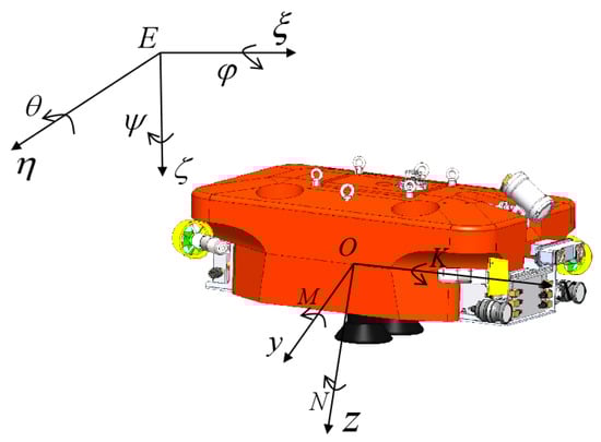
Figure 2.
ROV Earth-fixed coordinate frame and body-fixed coordinate frame.
The nonlinear dynamic equations of ROV are widely described using the Newton–Euler method in most studies [25], as follows:
where is the inertia matrix, is the Coriolis and centripetal matrix, is the damping matrix, and is the restoring moment matrix. represents the ROV’s position and orientation in . represents the ROV’s linear and angular velocities in . is the force and torque applied by the thrusters, and represents external disturbances such as wind, waves, and currents.
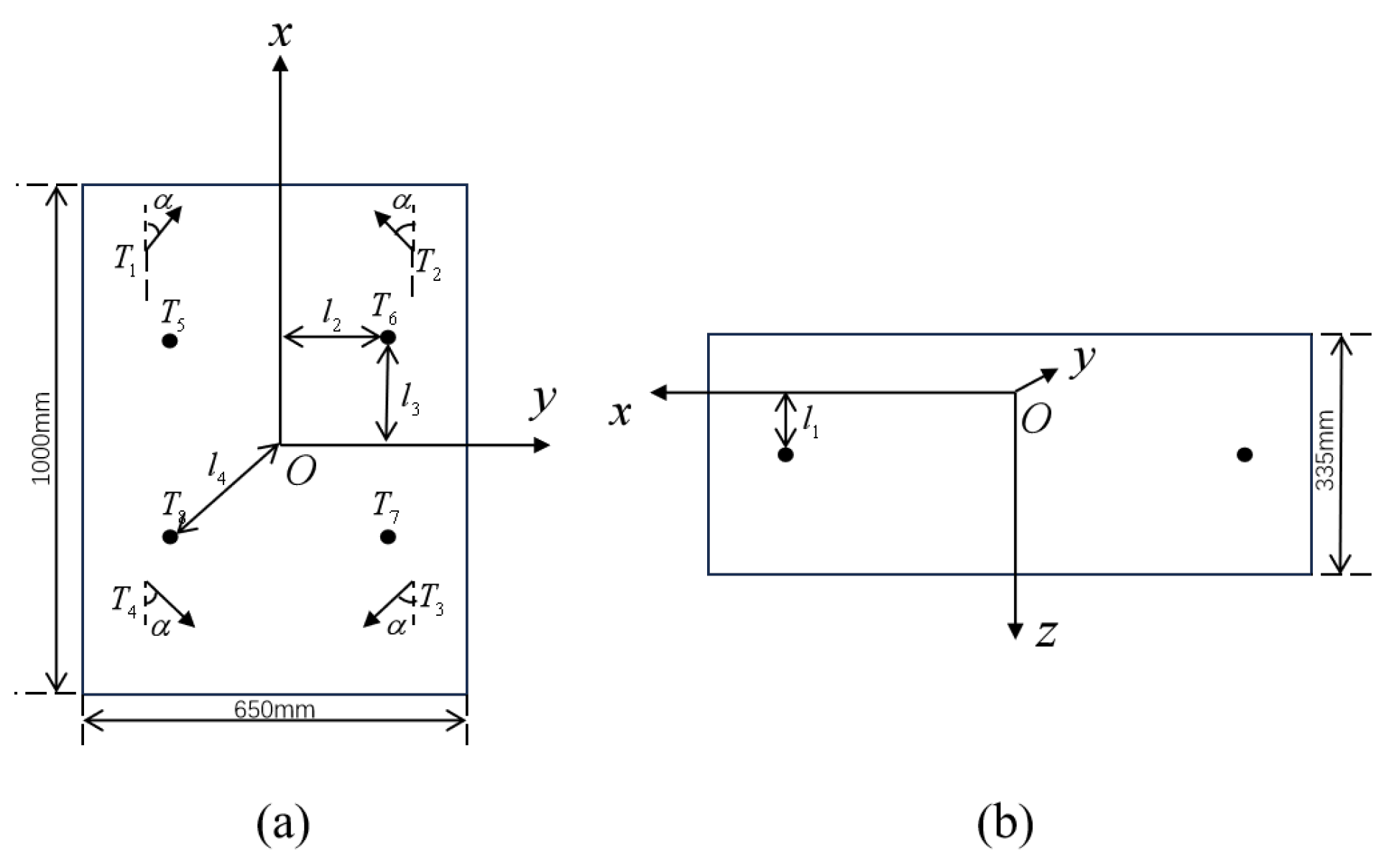
The ROV used in this study is the “R-ROV” [26] independently developed by the Shenyang Institute of Automation, Chinese Academy of Sciences. It is in a floating state in water and generates the required forces and moments in six degrees of freedom (DOFs) using eight thrusters. The thruster distribution is shown in Figure 3, providing dimensional data for the “R-ROV” simulation in WEBOTS.
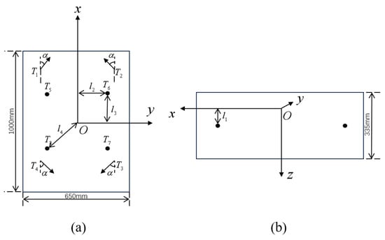
Figure 3.
“R-ROV” thruster distribution. (a) Top. (b) Side.
The relationship between the applied by the thrusters on the “R-ROV” and the T of each individual thruster is expressed as follows:
In Equation (3), represent the thrust of the eight thrusters distributed on the “R-ROV”. In Equation (2), is the thrust allocation matrix, expressed as follows:
where represent the angle between the horizontal thrusters and the of the ROV’s body-fixed coordinate system, the distance between the horizontal thrusters and the plane, the moment arm of the vertical thrusters relative to the , the moment arm of the vertical thrusters relative to the , and the moment arm of the horizontal thrusters relative to the , respectively.
4. GFSMO-NMPC Controller Design
Figure 4 shows the control framework. The GFSMO-NMPC controller consists of a Gaussian Function-based Sliding Mode Observer (GFSMO) and a Nonlinear Model Predictive Controller (NMPC). After the ROV locates its own state and the AUV’s state information through sensors, it calculates the pose error between them. Based on the three-stage docking control strategy, the ROV’s desired state is determined, and the GFSMO estimates the ROV’s predictive model compensation term. The NMPC performs rolling optimization based on the ROV’s desired state, the compensated predictive model, and model constraints to derive the predictive control sequence. Judging whether the predictive control sequence meets the optimal solution or reaches the maximum number of iterations, the optimal control sequence is output [27] to drive the ROV to approach the AUV.
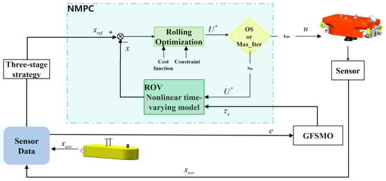
Figure 4.
GFSMO-NMPC control framework.
4.1. NMPC
The predictive model is the foundation of the NMPC controller. Constructing an accurate ROV model is difficult, and as the dimensionality of the predictive model increases, the computational pressure of NMPC significantly increases. To address this issue, the following reasonable assumptions are made:
- The ROV’s roll and pitch motions are ignored since the ROV relies on physical design (metacentric height) to maintain roll and pitch stability during active docking tasks.
- The Coriolis and centripetal matrix is ignored. Since the ROV operates at low speeds (less than 2 kn) during docking tasks, the influence of the Coriolis and centripetal matrix is proportional to the square of the velocity. Calculations show that the Coriolis moment accounts for less than of the main control moment at these speeds, so ignoring this term does not significantly affect modeling accuracy [28].
Based on these assumptions, and referring to the existing parameters of the “R-ROV” system and the ROV dynamic model (1) in Section 3, the state variables of the ROV are selected as , where , , and the control input . The constructed NMPC predictive model is as follows:
where is the Jacobian matrix corresponding to each moment, defined as in Equation (6), and the simplified mass matrix M and damping matrix are defined as in Equation (7).
where m is the ROV mass and is the rotational inertia of the ROV. and are the hydrodynamic coefficients of the ROV.
The 4th-order Runge–Kutta (RK4) method [23] is used to approximate the solution of the differential Equation (5). Within a small discrete time step , the ROV’s state at the next time step is obtained as shown in Equation (8).
The NMPC optimizes the cost function based on the ROV’s system state, desired state, and constraints. In the docking task, the primary considerations are the position error between the ROV and AUV and docking safety. The predicted state sequence and the control sequence are selected and the cost function is constructed as in Equation (9).
where is the prediction horizon, is the control horizon, Q is the state weight matrix, R is the control weight matrix, is the weight coefficient, and is the relaxation factor.
The constraints are related to the ROV’s physical limitations and task requirements, expressed as follows:
where Equation (10) is the dynamic constraint of the ROV, Equations (11) and (12) are the input and input increment constraints, and Equation (13) is the state constraint.
Through the predictive model (5) and cost function (9), the optimal control sequence (14) is derived within each control cycle, and the first control input is applied to the ROV. The optimal control input is transformed into individual thruster commands through multiplication with , the pseudo-inverse of the control effectiveness matrix . This computation yields the required thrust for each thruster, driving the ROV toward the target position.
4.2. GFSMO
A sliding mode observer-based feedback compensation mechanism is introduced [29] to reduce the NMPC controller’s dependence on the model. The sliding mode observer has transient response characteristics, quickly converging the observation error between the ROV’s actual state and desired state to zero, thereby dynamically compensating the NMPC’s predictive model.
The original sliding surface is defined as follows:
where , is the desired ROV state and x is the actual ROV state.
The original sliding surface (15) does not consider the limitation of the integral term, leading to excessive cumulative errors during the initial motion stage (when errors are typically large), causing lag and overshoot in the ROV’s motion. To address this issue, a sliding surface based on Gaussian function is introduced, replacing the original integral term with a Gaussian distribution curve, as shown in Figure 5.
where is the maximum value of the mapping interval, is the center value, and is the standard variance.
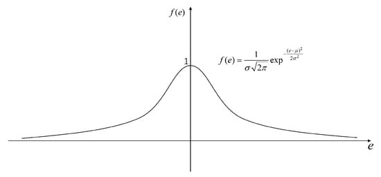
Figure 5.
Gaussian function.
The sliding surface based on the Gaussian function is defined as Equation (17):
With the introduction of a sliding mode surface based on the Gaussian function, it becomes an integral over , where the interval range of is . This method not only ensures the transient response characteristics of the sliding mode observer but also solves the overshooting and hysteresis problems.
The GFSMO is designed as follows:
where is the sliding mode gain, is the adaptive gain, and is the sign function on the sliding surface. By adjusting and , the ROV can estimate model uncertainties and unknown disturbances.
5. Simulations and Analysis
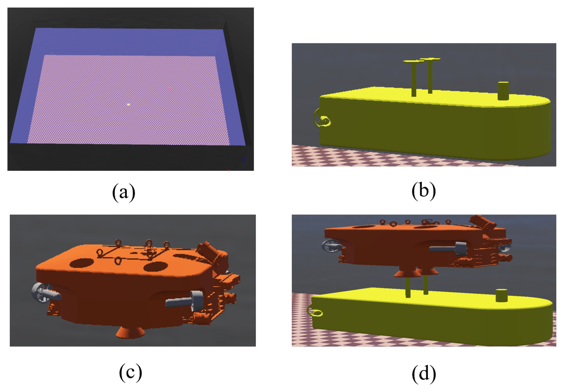
In this section, a joint simulation experiment using MATLAB and WEBOTS is conducted. MATLAB is responsible for writing the robot control program and data visualization, while WEBOTS handles the ROV’s dynamic simulation and visual simulation. The two platforms interact through the “Remote API” to collaboratively verify the feasibility of the GFSMO-NMPC control method and the three-stage docking control strategy. WEBOTS is a widely used open-access simulation platform for robotics, supporting underwater environments, underwater robot setup, and current disturbance settings. The simulation environment comprises a water tank with dimensions of 100 m (length) × 50 m (width) × 20 m (depth), into which the “R-ROV” and AUV models are integrated to accurately simulate the docking procedure. The simulation environment is shown in Figure 6.
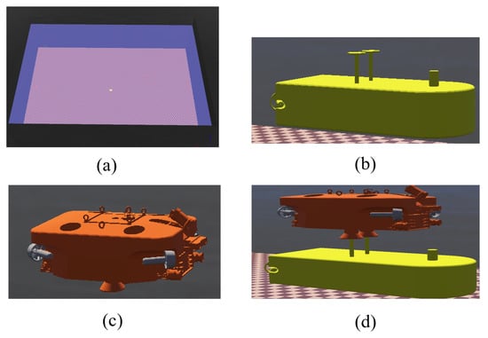
Figure 6.
WEBOTS simulation. (a) Pool. (b) AUV. (c) ROV. (d) Docking.
In WEBOTS, the relationship between the thrust generated by the thrusters and the motor speed is as follows:
where represents the thrust of the 8 thrusters of the ROV in Equation (3), k is a coefficient related to the shape, size, and fluid density of the thrusters, and for simplicity, in this paper. n is the rotational speed applied to the thruster motor.
The hydrodynamic parameters and mass of the robot in WEBOTS are modified according to Table 1 to simulate the hydrodynamics of “R-ROV”. Here, “dragForceCoefficients” and “dragTorqueCoefficients” represent the drag force and drag torque coefficients in three directions, respectively, and “viscousResistanceTorqueCoefficient” represents the viscous resistance coefficient.

Table 1.
‘ImmersionProperties’ setting.
In MATLAB, the NMPC predictive model shown in Equation (5) is constructed according to Table 2, and the parameters in the thrust allocation matrix (4) of the “R-ROV” are set according to Table 3.
Table 2.
Parameters of the ‘R-ROV’.
Table 3.
Parameters of the “R-ROV” thruster distribution.
Here, the “Supervisor” function in WEBOTS is used to replace localization sensors such as USBL and a binocular camera, enabling the simulation to obtain the position and orientation information of the ROV and AUV in the Earth-fixed coordinate system . Four different simulation scenarios are designed as follows:
Scenario 1: 3D trajectory tracking under disturbance; the tracking trajectory is given by Equation (20), with a simulation duration of 96 s and a simulation step size of T = 32 ms.
where represents the desired trajectory of the ROV, and represents the initial position of the ROV.
Scenario 2: docking with a floating AUV without disturbance; the motion trajectory of the AUV is given by Equation (21), with a maximum simulation duration of 30 s and a simulation step size of T = 32 ms.
where represents the motion trajectory of the AUV, and represents the initial position of the AUV.
Scenario 3: docking with a moving AUV without disturbance; the motion trajectory of the AUV is given by Equation (22), with a maximum simulation duration of 50 s and a simulation step size of T = 32 ms.
where represents the motion trajectory of the AUV, and represents the initial position of the AUV.
Scenario 4: docking with a moving AUV under disturbance; the motion trajectory of the AUV is given by Equation (23), with a maximum simulation duration of 50 s and a simulation step size of T = 32 ms.
where represents the motion trajectory of the AUV, represents the initial position of the AUV, and and represent the distances moved by the AUV in the longitudinal and lateral directions, respectively, due to stream velocity.
In practice, the success rate of ROV active docking with AUVs depends on the trajectory tracking performance of the ROV and the docking method. Therefore, Scenario 1 is designed with a nonlinear curve to verify the trajectory tracking performance of the proposed controller. Scenario 2 and Scenario 3 are designed to demonstrate the feasibility of ROV docking with a floating AUV and a moving AUV, respectively, without disturbance. Scenario 4 verifies the adaptability of the docking method under different current conditions by varying the stream velocity. The success mark for ROV-AUV docking task in Scenarios 2–4 are defined by the following: < 0.05 m and < 0.05 m and < 0.175 rad and −0.45 m < < −0.35 m.
5.1. Scenario 1
In WEBOTS, the simulation environment is initialized as follows: the initial position of the ROV is set to , with units in m. A constant stream velocity of m/s is applied. The NMPC parameters are configured as follows: prediction horizon , control horizon , and discrete time step s. The state weight matrix is , the control weight matrix is , the weight coefficient is set to 1, and the relaxation factor is set to 0.0001. In this paper, considering the temporary unavailability of the future trajectory of the AUV, the future reference trajectory of the NMPC at each sampling period , for all , where is the AUV state information collected at each sampling moment.
The GFSMO parameters are configured as follows: sliding mode gain and adaptive gain . Three algorithms are used to control the ROV to track the desired trajectory (20), and the results are shown in Figure 7.
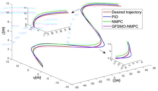
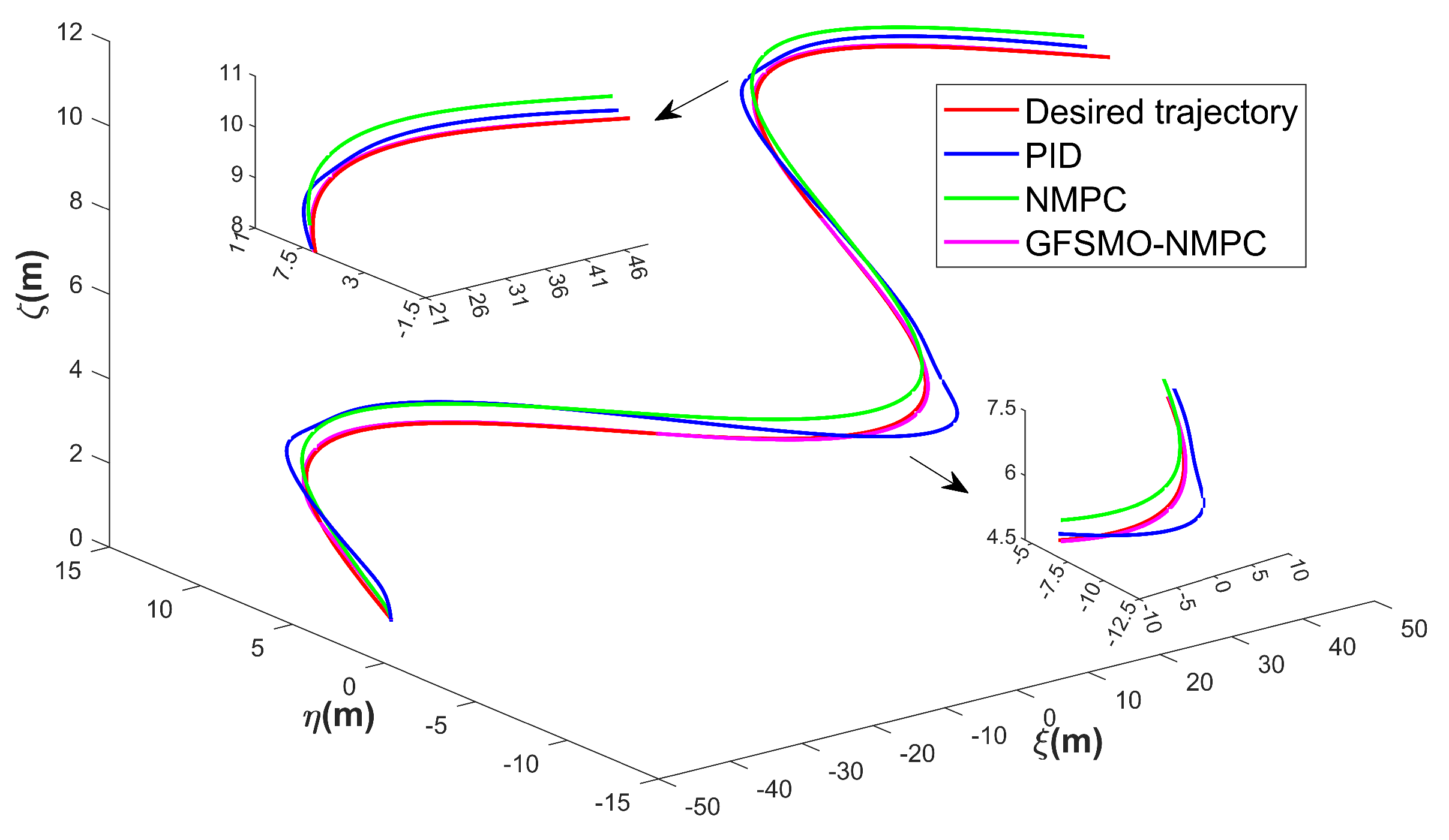
Figure 7.
ROV 3D trajectories for tracking under disturbances—Scenario 1.
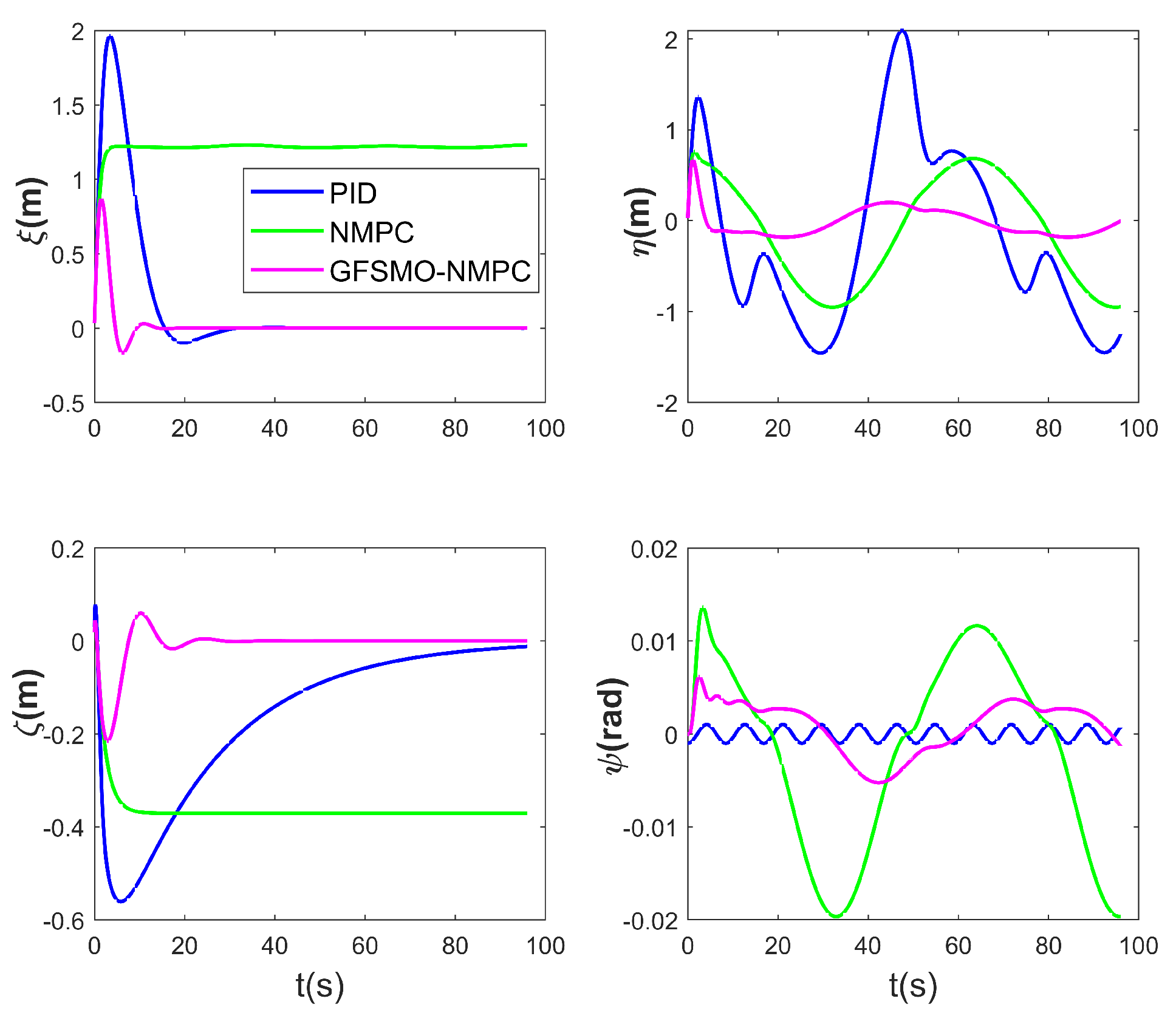
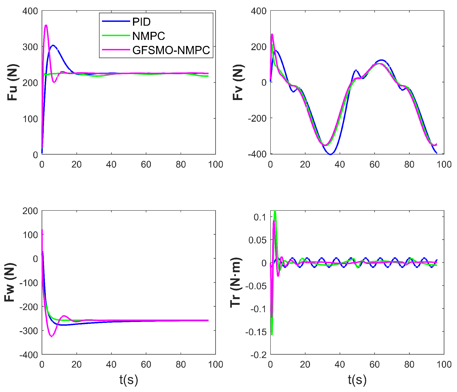
Figure 7, Figure 8, Figure 9 and Figure 10 present the simulation results of Scenario 1. The trajectory using GFSMO-NMPC is smoother than PID and NMPC, and the ROV stabilizes on the desired trajectory after 16 s. Both PID and NMPC exhibit significant fluctuations during trajectory turns, with larger tracking errors in the direction. Figure 8 shows the states of the ROV at different times during the tracking simulation using the GFSMO-NMPC algorithm in WEBOTS. Figure 9 illustrates the changes in the ROV tracking error in the directions. It is clear that in the and directions, GFSMO-NMPC eliminates the steady-state error compared to NMPC, with maximum tracking errors not exceeding 0.8 m and 0.2 m, respectively. Figure 10 compares the variations in , showing that the proposed method suppresses control input chattering. To evaluate the superiority of the proposed method, the root mean square error (RMSE) of the position and orientation tracking for the three algorithms is compared, and the results are shown in Table 4. It is evident that the proposed method improves the trajectory tracking accuracy of the ROV, with RMSE values of 0.1300 m, 0.1554 m, 0.0416 m, and 0.0029 rad in the directions, respectively. The results demonstrate that the proposed method significantly enhances the accuracy and control robustness of tracking task.

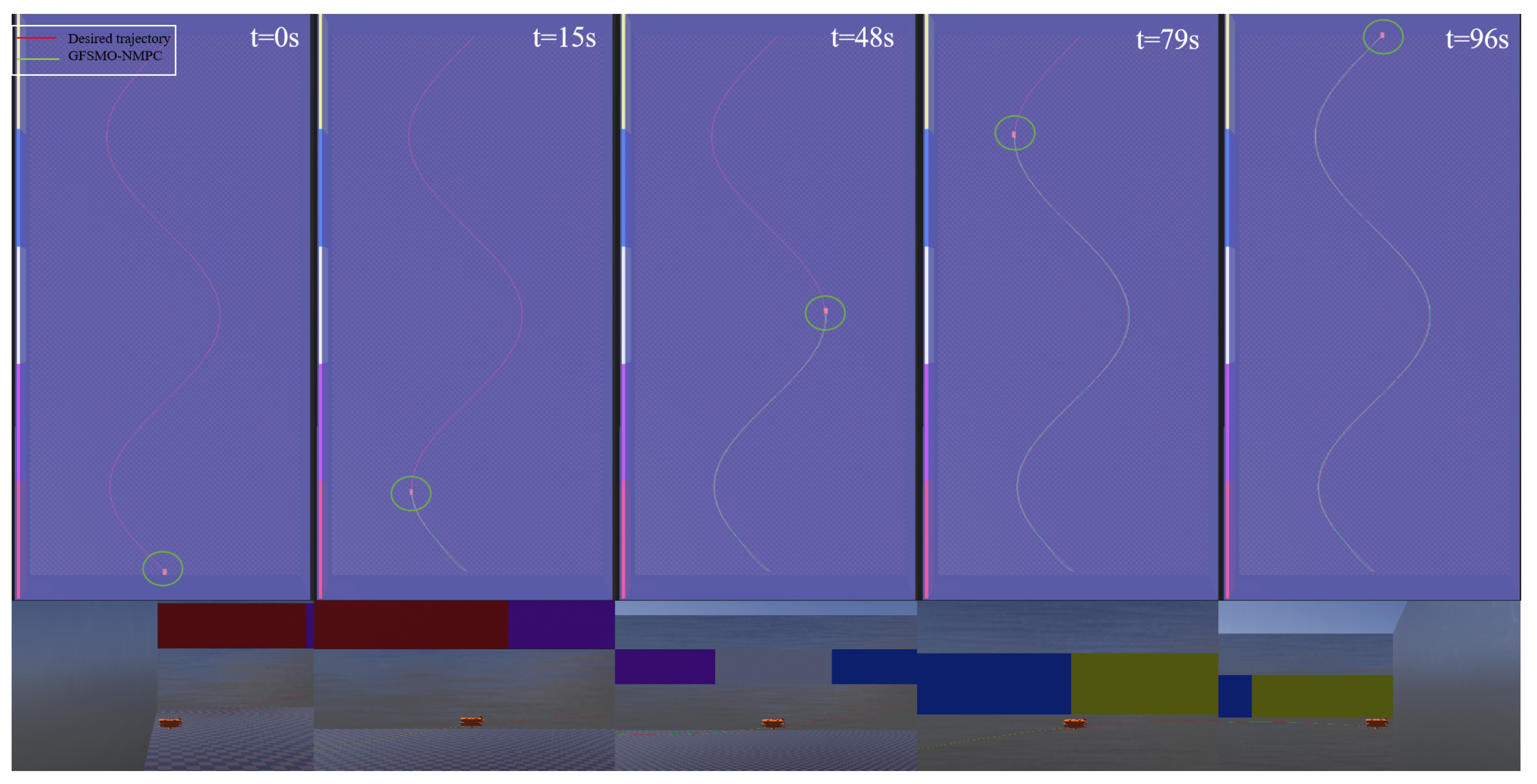
Figure 8.
ROV 3D trajectories visions for tracking based on GFSMO-NMPC—Scenario 1.
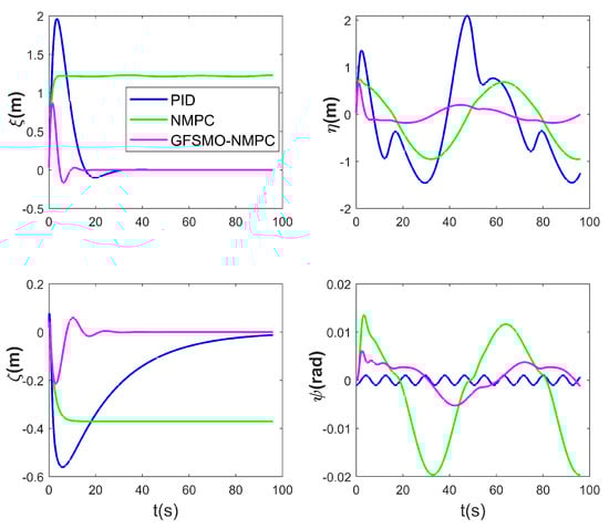
Figure 9.
ROV position and pose tracking errors for tracking under disturbances—Scenario 1.
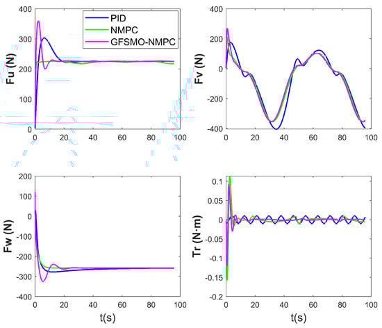
Figure 10.
The control input of ROV—Scenario 1.
Table 4.
The RMSE performance of different algorithms—Scenario 1.
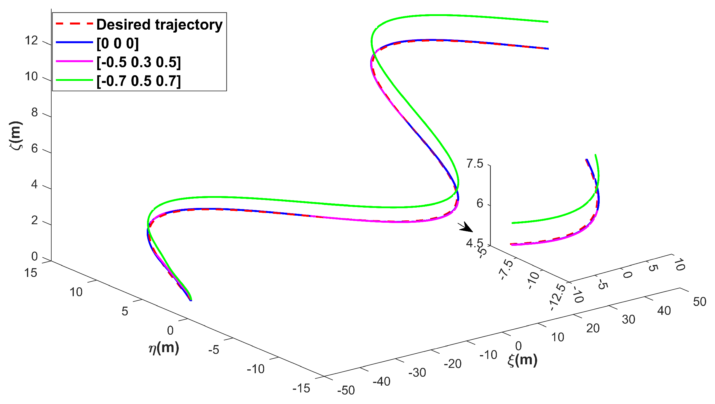
In order to verify the anti-disturbance performance of the GFSMO-NMPC, the constant stream velocity in the WEBOTS was changed without changing the trajectory and controller parameters. The simulation results show that when the vertical stream velocity is greater than 0.5 m/s, the vertical direction will lose control. So, three sets of stream velocities , and were selected for comparison and the results are as follows:
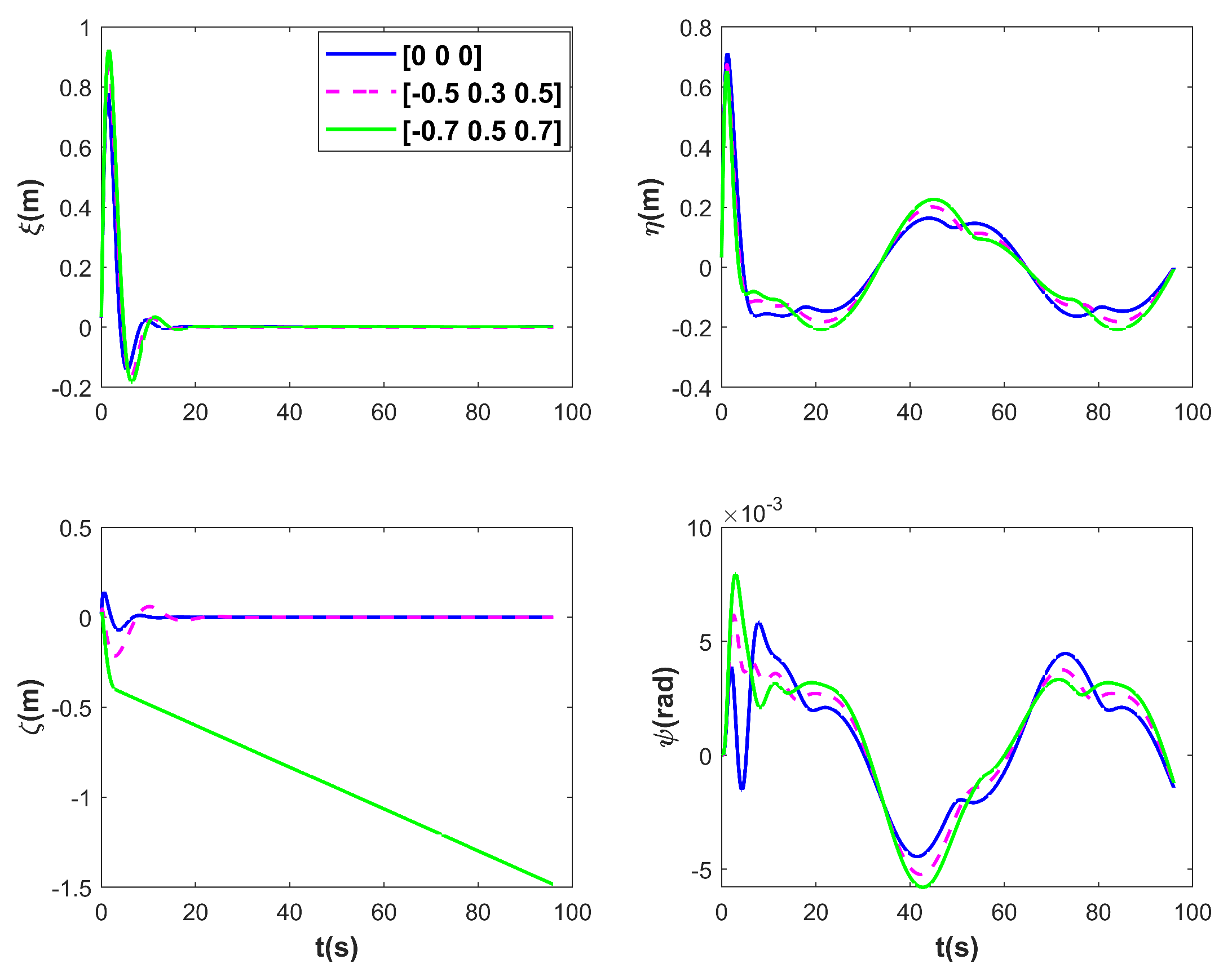
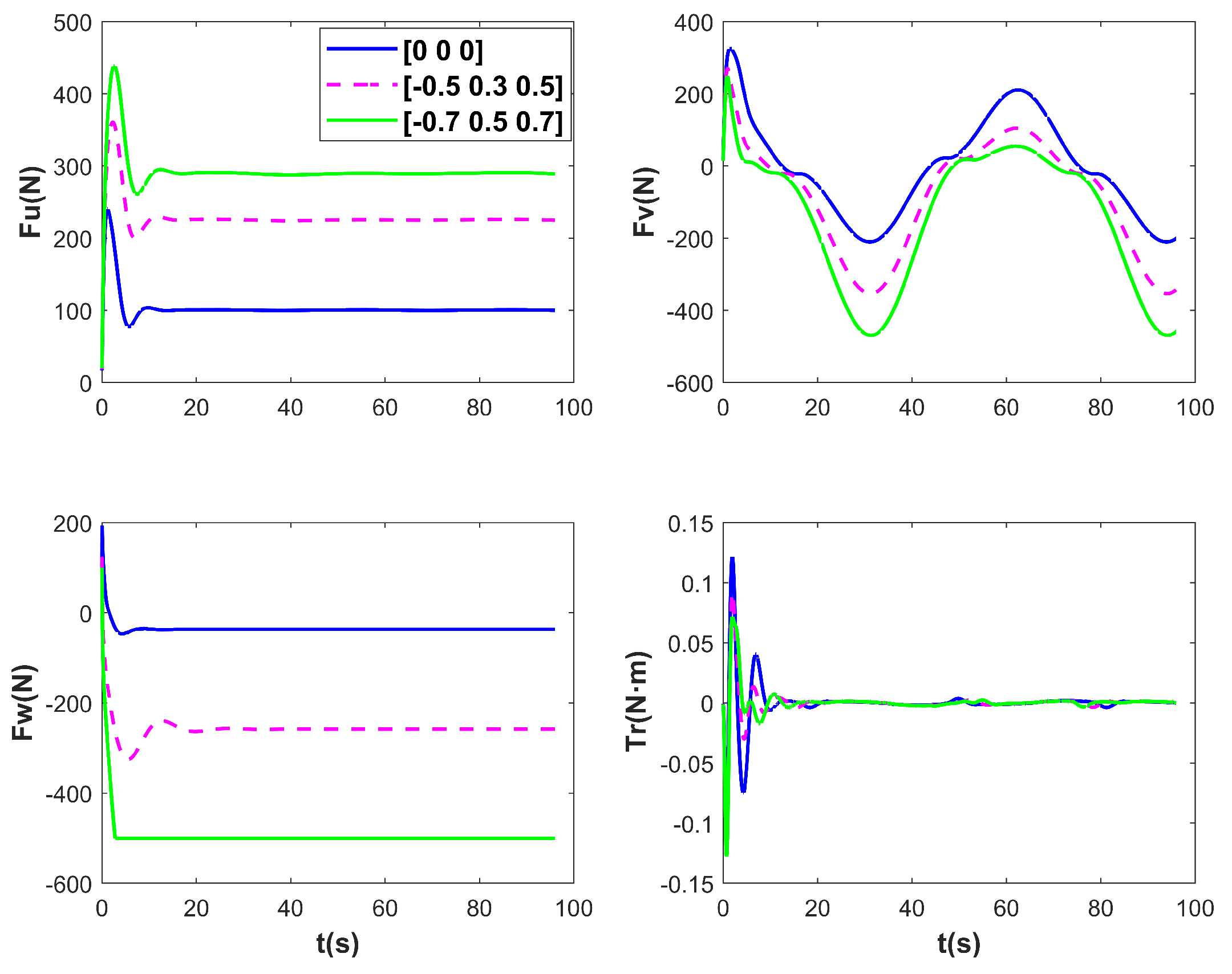
Figure 11, Figure 12 and Figure 13 present the simulation results of ROV 3D trajectories for tracking under different disturbances. Figure 11 visualizes the results of trajectory tracking, and it can be seen that the ROV tracking results are similar under both sets of disturbances, and . However, when the stream velocity increases to , the controller fails on . This is also reflected in the variation in Figure 13, when the ROV resists the upward current with maximum thrust, but still fails to track the desired trajectory. In Figure 12, it seems that as the current increases, it does not affect the tracking results in the and directions, as well as in the attitude, with the ROV tracking the desired trajectory steadily after 10 s. However, in Figure 13, it can be seen that as the stream velocity increases, the thrust/torque required by the ROV increases. For example, the stabilized thrust changes from 100 N to 210 N, and the final 290 N in the case of . It should be noted that the controller losses control on because the ROV still has to overcome the effects of buoyancy. The RMSEs under the three disturbances are compared in Table 5. The results demonstrate that the proposed method is robust.
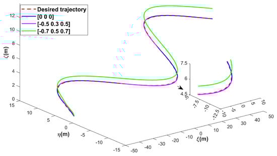
Figure 11.
ROV 3D trajectories for tracking under different disturbances.
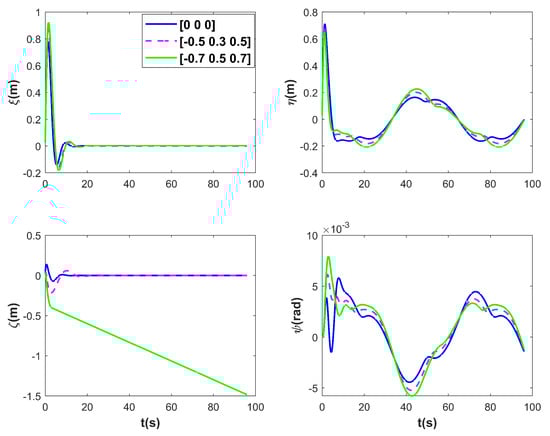
Figure 12.
ROV position and pose tracking errors for tracking under different disturbances.
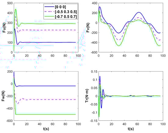
Figure 13.
The control input of ROV under different disturbances.
Table 5.
The RMSE performance of different disturbances.
5.2. Scenario 2
In WEBOTS, the initial positions of the ROV and AUV are set as follows: to be and to be ; the unit is m. The three-stage control strategy mentioned in Section 2 is adopted, and the AUV follows the trajectory specified in Equation (21). The GFSMO-NMPC parameter settings remain unchanged. The results are shown in Figure 14.
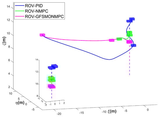
Figure 14.
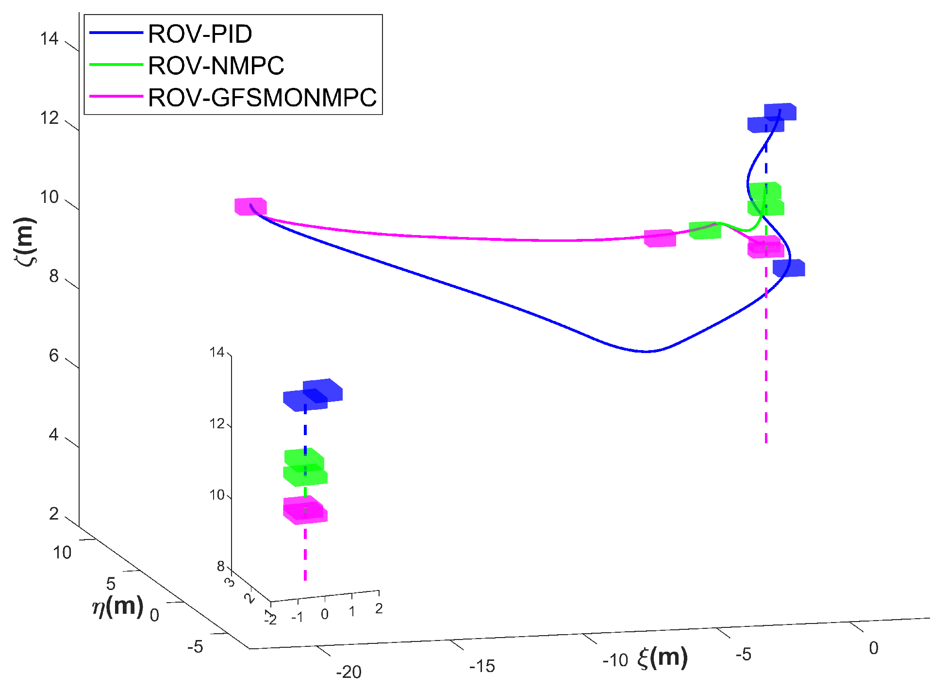
ROV 3D trajectories for docking unpowered AUVs—Scenario 2.
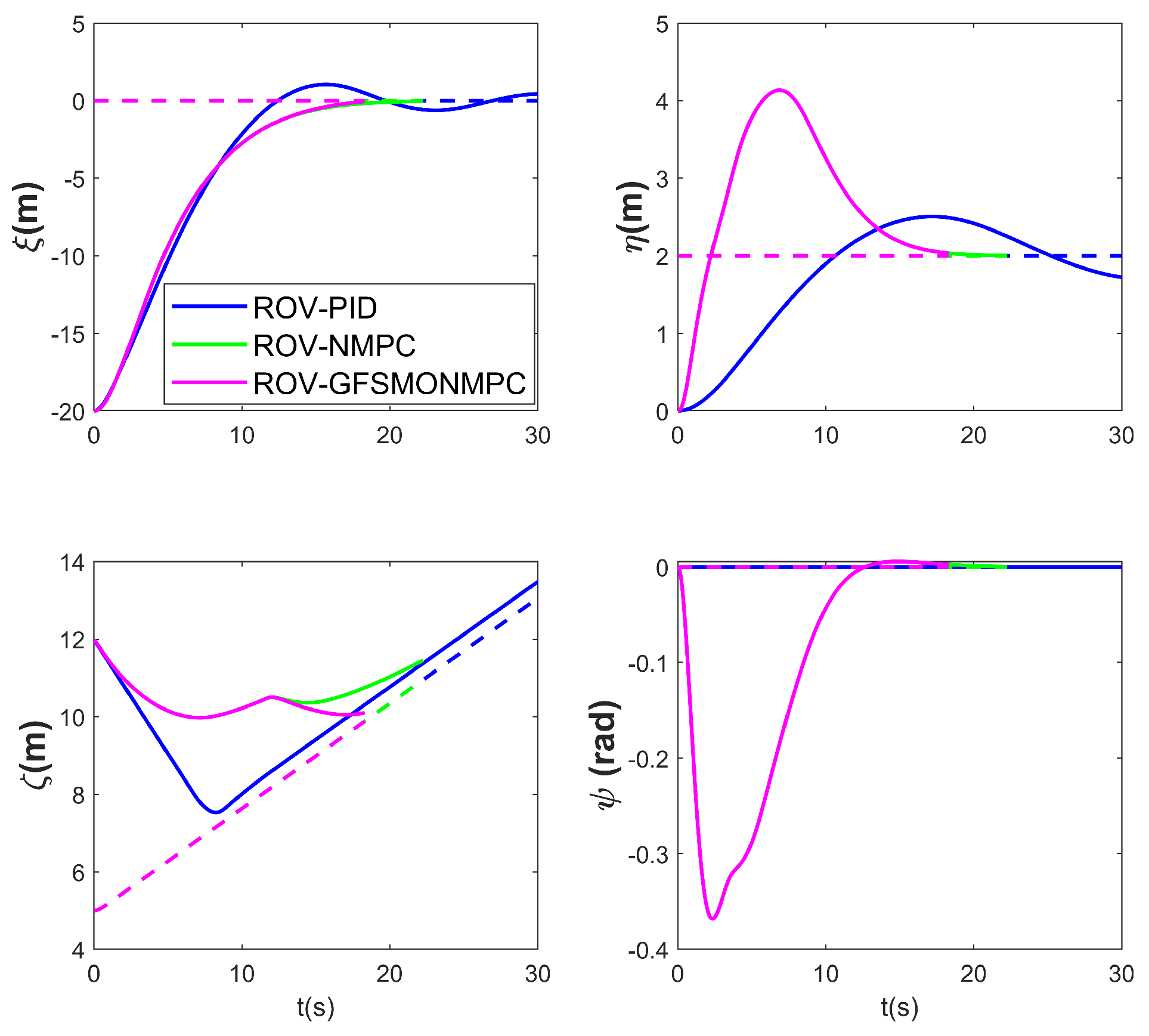
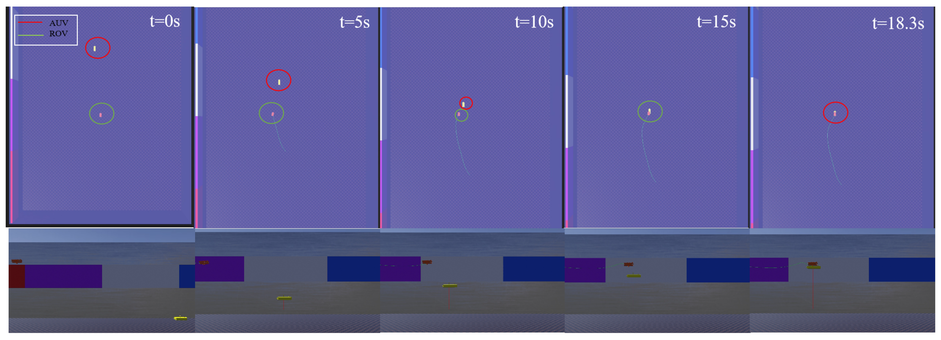
Figure 14, Figure 15 and Figure 16 present the simulation results of the ROV docking with a floating AUV without propulsion in Scenario 2. The simulation results demonstrate that the ROV successfully completed the docking task with the AUV in 18.3 s by implementing the proposed three-stage control strategy integrated with the GFSMO-NMPC algorithm. In contrast, the NMPC algorithm requires 22.24 s to complete the task. Although the PID algorithm allows the ROV to adjust to the same depth as the AUV in a shorter time, its lower control precision prevents it from completing the docking within 30 s. Figure 15 shows the changes in the position and orientation of the ROV during the docking process with the floating AUV. In the direction, overshoot occurs when using the proposed method. Through trajectory analysis in the WEBOTS, the phenomenon primarily stems from the directional coupling of the ROV. This occurs when uniform state weight coefficients are maintained in the Q matrix across all DOFs. Although the coupling effects between system states restrict the independent adjustment of weight coefficients due to potential instability risks, this limitation can be effectively mitigated through the implementation of advanced trajectory-planning techniques. Figure 16 shows the relative position between the ROV and the AUV during the docking simulation of Scenario 2 with the proposed method in WEBOTS.
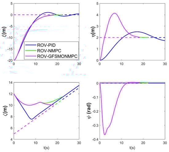
Figure 15.
ROV position and pose tracking performance for docking unpowered AUVs—Scenario 2.
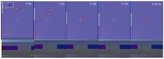
Figure 16.
ROV and AUV relative positions for docking unpowered AUVs—Scenario 2.
Table 6 compares the terminal position and orientation errors between the ROV and AUV, as well as the docking time, at the end of the simulation for Scenario 2 using the three methods. The terminal errors in the direction are similar for all methods. In the horizontal plane, the PID algorithm exhibits oscillations, preventing the ROV from stabilizing within the “steady-state circle”, with a deviation of 0.44 m in the direction and a lag of 0.276 m in the direction relative to the AUV’s docking interface. In contrast, both the NMPC and GFSMO-NMPC algorithms can stabilize within the “steady-state circle”. As for the yaw angle , all three methods show minor fluctuations, but these do not affect the final results and can be ignored.
Table 6.
The performance of different algorithms—Scenario 2.
5.3. Scenario 3
The initial positions of the ROV and AUV remain the same as in Scenario 2. The AUV follows the trajectory specified in Equation (22), and the parameter settings remain unchanged, except for the maximum docking time, which is set to 50 s. The results are shown in Figure 17.
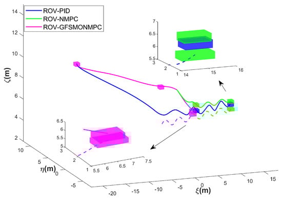
Figure 17.
ROV 3D trajectories for docking a moving AUV—Scenario 3.
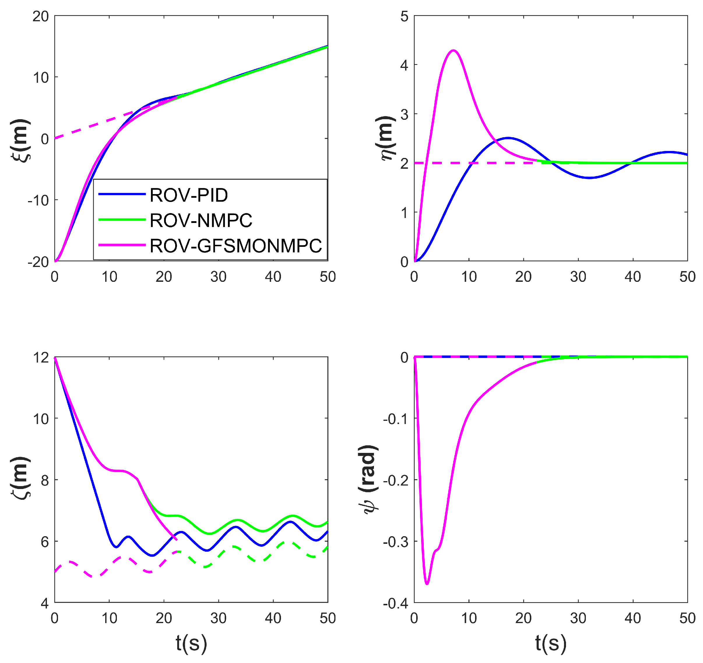
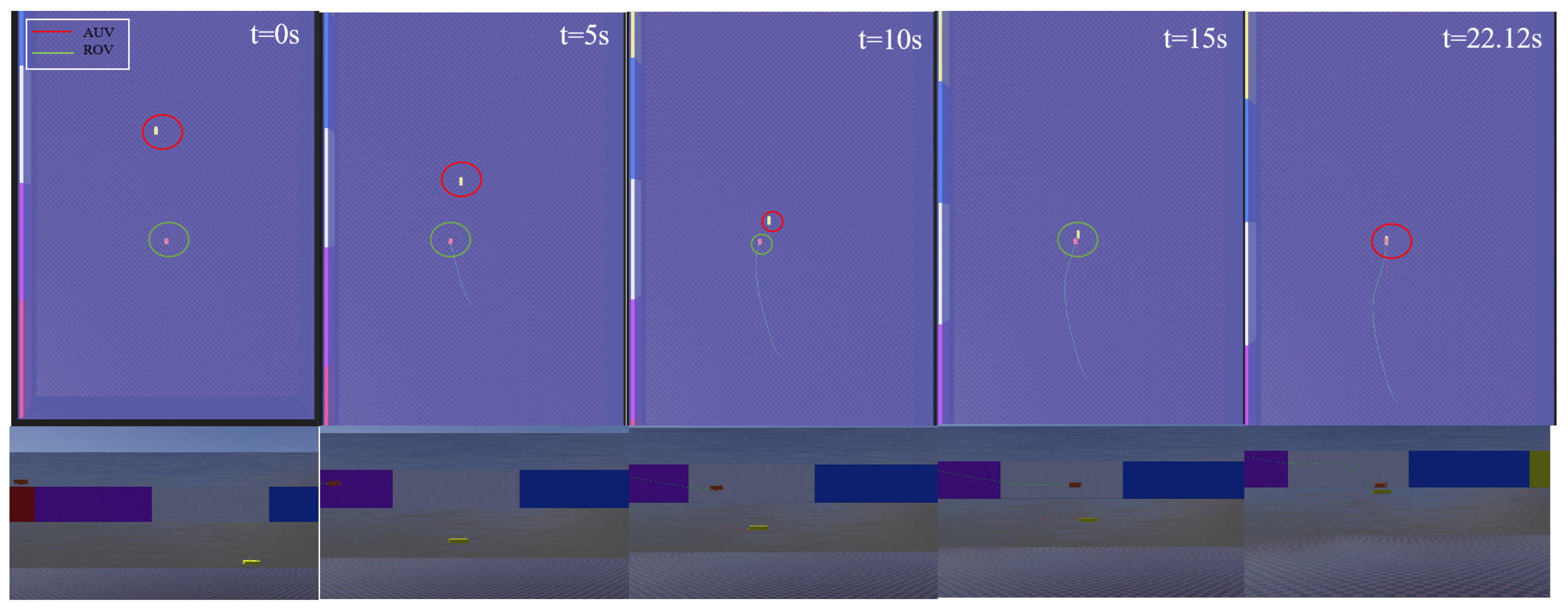
Figure 17, Figure 18 and Figure 19 present the simulation results of the ROV docking with a moving AUV in Scenario 3. The results clearly demonstrate the superiority of the proposed method, as the ROV successfully docks with the AUV in 22.12 s. In contrast, both the NMPC and the PID algorithms fail to complete the docking task within 50 s. This result indicates that the proposed method remains feasible even when the AUV moves. Figure 18 shows the changes in the position and orientation of the ROV during the docking process with the moving AUV. Similar to the case of docking with a floating AUV, an overshoot issue occurs in the direction, with a maximum overshoot of 2.3 m. Figure 19 shows the relative position between the ROV and the AUV during the docking simulation of Scenario 3 with the proposed method in WEBOTS.

Figure 18.
ROV position and pose tracking performance for docking a moving AUV—Scenario 3.
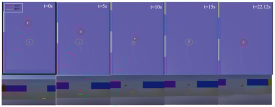
Figure 19.
ROV and AUV relative positions for docking a moving AUV—Scenario 3.
Table 7 compares the terminal position and orientation errors between the ROV and AUV, as well as the docking time, at the end of the simulation for Scenario 3 using the three methods. The ROV using the PID and NMPC algorithms has terminal errors in the direction, and the PID algorithm predicts oscillations in both the and directions. Overall, the proposed method demonstrates feasibility in the docking task.
Table 7.
The performance of different algorithms—Scenario 3.
5.4. Scenario 4
After fixing the parameters of the GFSMO-NMPC algorithm, nine docking simulations are conducted with different stream velocities while keeping the initial positions of the ROV and AUV unchanged. The AUV follows the trajectory specified in Equation (23), and the results are combined with the special case of no current in Scenario 3. The terminal position and orientation errors between the ROV and the AUV, as well as the docking time, are compared, and the results are shown in Table 8.
Table 8.
The performance of ROV docking a moving AUV under changed disturbances—Scenario 4.
An important limitation to consider is that the stream velocity is fixed in WEBOTS. However, the current is random in the real world. In this study, ten docking simulations with varying horizontal stream velocities were conducted to investigate the effects of stochastic hydrodynamic disturbances on docking performance under real-world conditions. The results show that the proposed method achieves a docking success rate of .
In Table 8, it can be seen that as the stream velocity increases, the docking time also increases. The docking time reaches its minimum when the stream velocity is 0 m/s. Since no current is set in the direction, does not change significantly compared to the no-disturbance condition. In the horizontal plane, influenced by the stream velocity, is larger when the ROV moves against the flow (−1 to 0 m/s) than when it moves with the flow (0 to 1 m/s). When the stream velocity exceeds 1 m/s (2 kn), the ROV’s maneuverability is affected, making it difficult to complete the docking with the AUV. At a stream velocity of 1.1 m/s, the docking is completed in 36.32 s. However, when the stream velocity reaches 1.4 m/s, the docking task fails. These results indicate that the proposed method has disturbance rejection capability and is suitable for ROV-AUV docking tasks within a small stream velocity range (−1 to 1 m/s).
6. Experimental Guide
To provide a clear understanding of the physical implementation of the proposed method, this section introduces the R-ROV platform, followed by the experimental protocols. The R-ROV platform (Figure 20) integrates a dual-sensor system for self-localization and target localization and employs two computing units.
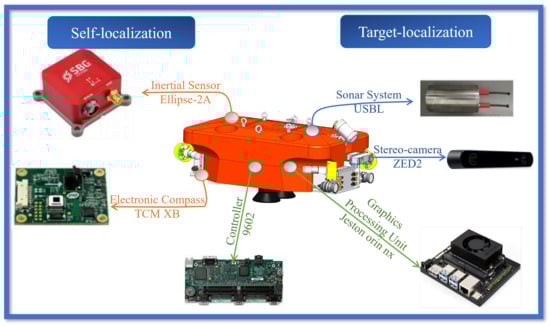
Figure 20.
R-ROV test platform.
On the self-localization hand, the Ellipse-2A inertial sensor provides 6-DoF kinematic data (linear acceleration, angular velocity, and attitude). The TCM XB electronic compass calibrates the heading angle of the Ellipse-2A to ensure yaw accuracy. On the target localization hand, a USBL sonar system acquires the target’s positional coordinates. A ZED2 binocular camera estimates the target’s 6-DoF pose (position and orientation). In addition, the platform employs a 9602 calculator for sensor data fusion, motion control, and thruster actuation. A dedicated Jetson Orin NX GPU is used for real-time visual processing. With a total mass of 170 kg, the R-ROV demonstrates robust self/target localization capabilities underwater.
The guidelines for the experiment are as follows:
- Pre-dive inspection: Verify the watertight integrity of the R-ROV and target AUV. Calibrate all sensors.
- Task initialization: Configure the AUV’s operational mode via the surface console (constant-speed cruising at 1 kn or station-keeping with ±0.1 m positional tolerance). Initialize the R-ROV docking mission parameters.
- System deployment: Deploy the R-ROV and target AUV into the water using a crane, maintaining a horizontal separation of 20 m.
- Long-distance approach: Activate the USBL system on the R-ROV. Navigate toward the hovering offset point S using USBL-derived coordinates.
- Sensor transition: When the Euclidean distance satisfies , deactivate the USBL system. Enable the ZED2 binocular camera for vision-based localization.
- Relative hovering: Converge into the steady-state circle around point S using real-time pose data from the binocular camera. Maintain horizontal tracking errors within < 0.05 m & < 0.05 m.
- Hovering validation: Synchronize horizontal motion with the AUV for 1 min within the steady-state circle. Log telemetry data (position, orientation, thrust) for offline analysis.
- Contact docking: Disable hovering control once stabilized within the circle. Initiate vertical descent toward the AUV until physical contact is achieved.
- Recovery and analysis: Synchronize the ascent of the R-ROV and AUV to the surface. Retrieve both vehicles via crane; inspect docking mechanism wear and clean optical sensors. Process logged data to compute performance metrics.
In the real word, overshooting and hysteresis may occur in the R-ROV due to the model uncertainty of the R-ROV and the disturbance of the current. It is necessary to set the R-ROV remote control maneuvering mode to start the remote control maneuvering mode to drive the R-ROV away from the docking area when the R-ROV and the AUV are about to collide, and adjust the control parameters in time for the secondary docking test.
7. Conclusions
This study proposes a control method for Remotely Operated Vehicles (ROVs) to actively dock with AUVs, to address the limitations of traditional docking and recovery schemes for Autonomous Underwater Vehicles (AUVs), such as restricted maneuverability and external disturbances. A process and control strategy for ROV active docking with AUVs is designed, dividing the docking process into long-distance approach, relative hovering, and contact docking stages based on the Euclidean distance between the ROV and AUV. An NMPC algorithm is used as the ROV’s motion controller, and a GFSMO is introduced to compensate for the predictive model, eliminating steady-state errors during the ROV’s motion.
In the simulation experiments, the GFSMO-NMPC algorithm demonstrated strong robustness in trajectory tracking tasks compared to PID and the original NMPC, with RMSE values of 0.1300 m, 0.1554 m, 0.0416 m, and 0.0029 rad in four DOFs, and discuss the performance of controller under different disturbances. In the docking experiments, the ROV successfully docked with both stationary and moving AUVs, with docking times of 18.3 s and 22.12 s, respectively. After optimizing the controller parameters, the docking success rate reached in 10 docking experiments under varying stream velocity. These results indicate that the proposed controller and method are suitable for docking tasks. Finally, we introduced the “Experimental guides”.
Future work will consider the impact of sensor measurement errors on the ROV’s self-localization and target AUV localization, and a trajectory prediction-based method will be used to guide the ROV toward the AUV. The method will also be tested in pool test using the “R-ROV”.
Author Contributions
Conceptualization, Q.Z., S.C. and Y.Z.; methodology, H.D. and Y.Z.; writing—original draft preparation, H.D.; writing—review and editing, H.D., S.C., Y.Z. and X.Z.; funding acquisition, Y.Z. All authors have read and agreed to the published version of the manuscript.
Funding
This research was funded by the National Natural Science Foundation of China (62403455), and the fundamental research project of SIA (2023JC3K05).
Data Availability Statement
The data can be obtained from the corresponding author.
Acknowledgments
Thanks to all the reviewers for their contributions to improving the quality of this paper.
Conflicts of Interest
The authors declare no conflicts of interest.
References
- Cai, W.; Tao, C.; Wang, Y.; Wu, T.; Xu, C.; Zhang, G.; Zhang, J.; Chen, Y. Applications of Autonomous Underwater Vehicle in Submarine Hydrothermal Fields: A Review. Robot 2023, 45, 483–495. [Google Scholar] [CrossRef]
- Zhou, J.; Si, Y.; Lin, Y.; Wei, Y.; An, X.; Wang, H.; Huang, H.; Chen, Y. A review of subsea AUV technology. Acta Oceanol. Sin. 2023, 45, 1119. [Google Scholar] [CrossRef]
- Liu, J.X.; Yu, F.; He, B.; Soares, C.G. A review of underwater docking and charging technology for autonomous vehicles. Ocean. Eng. 2024, 297, 117154. [Google Scholar] [CrossRef]
- Yazdani, A.M.; Sammut, K.; Yakimenko, O.; Lammas, A. A survey of underwater docking guidance systems. Robot. Auton. Syst. 2020, 124, 103382. [Google Scholar] [CrossRef]
- Chon, S.J.; Kim, J.Y.; Choi, H.S.; Kim, J.H. Modeling and Implementation of Probability-Based Underwater Docking Assessment Index. J. Mar. Sci. Eng. 2023, 11, 2127. [Google Scholar] [CrossRef]
- Allen, B.; Austin, T.; Forrester, N.; Goldsborough, R.; Kukulya, A.; IEEE. Autonomous docking demonstrations with enhanced REMUS technology. In Proceedings of the Oceans 2006 Conference, Boston, MA, USA, 18–21 September 2006; pp. 1–6. [Google Scholar] [CrossRef]
- Liu, S.; Xu, H.; Lin, Y.; Gao, L. Visual Navigation for Recovering an AUV by Another AUV in Shallow Water. Sensors 2019, 19, 1889. [Google Scholar] [CrossRef]
- Zheng, R.; Lu, H.; Yu, C.; Han, X.; Li, M.; Wei, A. Technical Research, System Design and Implementation of Docking between AUV and Autonomous Mobile Dock Station. Robot 2019, 41, 713–721. [Google Scholar] [CrossRef]
- Yan, Z.P.; Gong, P.; Zhang, W.; Li, Z.X.; Teng, Y.B. Autonomous Underwater Vehicle Vision Guided Docking Experiments Based on L-Shaped Light Array. IEEE Access 2019, 7, 72567–72576. [Google Scholar] [CrossRef]
- Yan, Z.P.; Xu, D.; Chen, T.; Zhou, J.J.; Wei, S.L.; Wang, Y.Z. Modeling, Strategy and Control of UUV for Autonomous Underwater Docking Recovery to Moving Platform. In Proceedings of the 36th Chinese Control Conference (CCC), Dalian, China, 26–28 July 2017; pp. 4807–4812. [Google Scholar] [CrossRef]
- Zhang, W.; Wu, W.H.; Teng, Y.B.; Li, Z.X.; Yan, Z.P. An underwater docking system based on UUV and recovery mother ship: Design and experiment. Ocean Eng. 2023, 281, 114767. [Google Scholar] [CrossRef]
- Huang, M.; Xu, J.; Shi, L. Application and prospect of rov in offshore oil and gas field development. Mar. Geol. Lett. 2021, 37, 77–84. [Google Scholar] [CrossRef]
- Song, J.; Liu, A.; Zhou, H.; Fu, J.; Mao, J. Applications of ROV for Underwater Inspection of Bridge Structures and Review of Its Anti-current Technologies. World Sci. Technol. Res. Dev. 2023, 45, 365–382. [Google Scholar] [CrossRef]
- Gray, A.C.; Schwartz, E.M. The NaviGator Autonomous Maritime System. Nav. Eng. J. 2017, 129, 75–88. [Google Scholar]
- Morinaga, A.; Nakano, T.; Kato, Y.; Uchihori, H.; Yamamoto, I. Development of a Docking Station ROV for Underwater Power Supply to AUVs. In Proceedings of the OCEANS Conference, San Diego, CA, USA, 20–23 September 2021. [Google Scholar] [CrossRef]
- Uchihori, H.; Yamamoto, I.; Morinaga, A. Concept of Autonomous Underwater Vehicle Docking Using 3D Imaging Sonar. Sens. Mater. 2019, 31, 4223–4230. [Google Scholar] [CrossRef]
- Trslic, P.; Rossi, M.; Robinson, L.; O’Donnel, C.W.; Weir, A.; Coleman, J.; Riordan, J.; Omerdic, E.; Dooly, G.; Toal, D. Vision based autonomous docking for work class ROVs. Ocean. Eng. 2020, 196, 106840. [Google Scholar] [CrossRef]
- Ji-yong, L.; Hao, Z.; Hai, H.; Xu, Y.; Zhaoliang, W.; Lei, W. Design and Vision Based Autonomous Capture of Sea Organism with Absorptive Type Remotely Operated Vehicle. IEEE Access 2018, 6, 73871–73884. [Google Scholar] [CrossRef]
- Mu, W.; Wang, Y.; Sun, H.; Liu, G. Double-Loop Sliding Mode Controller with An Ocean Current Observer for the Trajectory Tracking of ROV. J. Mar. Sci. Eng. 2021, 9, 1000. [Google Scholar] [CrossRef]
- Uchihori, H.; Cavanini, L.; Tasaki, M.; Majecki, P.; Yashiro, Y.; Grimble, M.J.; Yamamoto, I.; van der Molen, G.M.; Morinaga, A.; Eguchi, K. Linear Parameter-Varying Model Predictive Control of AUV for Docking Scenarios. Appl. Sci. 2021, 11, 4368. [Google Scholar] [CrossRef]
- Wu, W.; Zhang, W.; Du, X.; Li, Z.; Wang, Q. Homing tracking control of autonomous underwater vehicle based on adaptive integral event-triggered nonlinear model predictive control. Ocean. Eng. 2023, 277, 114243. [Google Scholar] [CrossRef]
- Zheng, X.; Xu, W.; Dai, H.; Li, R.; Jiang, Y.; Tian, Q.; Zhang, Q.; Wang, X. A coordinated trajectory tracking method with active utilization of drag for underwater vehicle manipulator systems. Ocean Eng. 2024, 306, 118091. [Google Scholar] [CrossRef]
- Anderlini, E.; Parker, G.G.; Thomas, G. Control of a ROV carrying an object. Ocean Eng. 2018, 165, 307–318. [Google Scholar] [CrossRef]
- Siciliano, B.; Khatib, O.; Kroger, T. Springer Handbook of Robotics; Springer: Berlin/Heidelberg, Germany, 2008; Volume 200. [Google Scholar]
- Fossen, T.I. Guidance and Control of Ocean Vehicles; John Wiley & Sons: Hoboken, NJ, USA, 1994. [Google Scholar]
- Zhang, Y.X.; Zhang, Q.F.; Zhang, A.Q.; Chen, J.; Li, X.; He, Z. Acoustics-Based Autonomous Docking for A Deep-Sea Resident ROV. China Ocean. Eng. 2022, 36, 100–111. [Google Scholar] [CrossRef]
- Rawlings, J.B.; Mayne, D.Q.; Diehl, M. Model Predictive Control: Theory, Computation, and Design; Nob Hill Publishing: Madison, WI, USA, 2017; Volme 2. [Google Scholar]
- Fossen, T.I. Handbook of Marine Craft Hydrodynamics and Motion Control; John Wiley & Sons: Hoboken, NJ, USA, 2011. [Google Scholar]
- Hong, H.C.; Yang, Z.Q.; Li, J.W.; Xu, G.H.; Xia, Y.K.; Xu, K. State-Transform MPC-SMC-Based Trajectory Tracking Control of Cross-Rudder AUV Carrying Out Underwater Searching Tasks. J. Mar. Sci. Eng. 2024, 12, 883. [Google Scholar] [CrossRef]


Disclaimer/Publisher’s Note: The statements, opinions and data contained in all publications are solely those of the individual author(s) and contributor(s) and not of MDPI and/or the editor(s). MDPI and/or the editor(s) disclaim responsibility for any injury to people or property resulting from any ideas, methods, instructions or products referred to in the content. |
© 2025 by the authors. Licensee MDPI, Basel, Switzerland. This article is an open access article distributed under the terms and conditions of the Creative Commons Attribution (CC BY) license (https://creativecommons.org/licenses/by/4.0/).