


Azimuthal Variation in the Surface Wave Velocity of the Philippine Sea Plate

Abstract
:1. Introduction
2. Data, Methodology, and Results
3. Interpretation and Discussion
4. Conclusions
Supplementary Materials
Funding
Data Availability Statement
Acknowledgments
Conflicts of Interest
References
- Corchete, V. Crust and upper mantle structure beneath the Yellow Sea, the East China Sea, the Japan Sea, and the Philippine Sea. Int. Geol. Rev. 2023, 65, 2594–2604. [Google Scholar] [CrossRef]
- Conrad, C.P.; Behn, M.D.; Silver, P.G. Global mantle flow and the development of seismic anisotropy: Difference between the oceanic and continental upper mantle. J. Geophys. Res. 2007, 112, B07317. [Google Scholar] [CrossRef]
- Liu, K.H.; Gao, S.S.; Gao, Y.; Wu, J. Shear-wave splitting and mantle flow associated with the deflected Pacific slab beneath northeast Asia. J. Geophys. Res. 2008, 113, B01305. [Google Scholar] [CrossRef]
- Corchete, V. Azimuthal variation in the surface-wave velocity in the Arabian plate. Appl. Sci. 2024, 14, 5142. [Google Scholar] [CrossRef]
- Isse, T.; Shiobara, H.; Montagner, J.-P.; Sugioka, H.; Ito, A.; Shito, A.; Kanazawa, T.; Yoshizawa, K. Anisotropic structures of the upper mantle beneath the northern Philippine Sea region from Rayleigh and Love wave tomography. Phys. Earth Planet. Inter. 2010, 183, 33–43. [Google Scholar] [CrossRef]
- Yeh, Y.; Kao, H.; Wen, S.; Chang, W.-Y.; Chen, C.-H. Surface wave tomography and azimuthal anisotropy of the Philippine Sea Plate. Tectonophysics 2013, 592, 94–112. [Google Scholar] [CrossRef]
- Corchete, V. Review of the methodology for the inversion of surface-wave phase velocities in a slightly anisotropic medium. Comput. Geosci. 2012, 41, 56–63. [Google Scholar] [CrossRef]
- Babuska, V.; Cara, M. Seismic Anisotropy in the Earth; Kluwer Academic: Dordrecht, The Netherlands, 1991. [Google Scholar]
- Corchete, V.; Badal, J. Inversion of surface wave phase velocities in a slightly anisotropic medium. Tecnociencia 2004, 6, 23–41. [Google Scholar]
- Corchete, V. Crust and upper mantle structure of Mars determined from surface-wave analysis. Earth Space Sci. 2024; submitted. [Google Scholar]
- Smith, L.M.; Dahlen, F.A. The azimuthal dependence of Love wave propagation in a slightly anisotropic medium. J. Geophys. Res. 1973, 78, 3321–3333. [Google Scholar] [CrossRef]
- Corchete, V.; Chourak, M.; Hussein, H.M. Shear wave velocity structure of the Sinai Peninsula from Rayleigh wave analysis. Surv. Geophys. 2007, 28, 299–324. [Google Scholar] [CrossRef]
- Louden, K.E. The crustal and lithospheric thicknesses of the Philippine Sea as compared to the Pacific. Earth Planet. Sci. Lett. 1980, 50, 275–288. [Google Scholar] [CrossRef]
- Huang, J.; Zhao, D. High-resolution mantle tomography of China and surrounding regions. J. Geophys. Res. 2006, 111, B09305. [Google Scholar] [CrossRef]
- Nicolas, A.; Christensen, N.I. Formation of anisotropy in upper mantle peridotites—A review. In The Composition, Structure and Dynamics of the Lithosphere-Asthenosphere System; Froidevaux, C., Fuchs, K., Eds.; AGU Geophysics Services: Washington, DC, USA, USA, 1987; Volume 16, pp. 111–123. [Google Scholar]
- Kawakatsu, H.; Kumar, P.; Takei, Y.; Shinohara, M.; Kanazawa, T.; Araki, E.; Suyehiro, K. Seismic evidence for sharp lithosphere-asthenosphere boundaries of oceanic plates. Science 2009, 324, 499–502. [Google Scholar] [CrossRef] [PubMed]
- Montagner, J.-P.; Tanimoto, T. Global upper mantle tomography of seismic velocities and anisotropies. J. Geophys. Res. 1991, 96, 20337–20351. [Google Scholar] [CrossRef]
- Maggi, A.; Debayle, E.; Priestley, K.; Barruol, G. Azimuthal anisotropy of the Pacific region. Earth Planet. Sci. Lett. 2006, 250, 53–71. [Google Scholar] [CrossRef]
- Plomerová, J.; Kouba, D.; Babuska, V. Mapping the lithosphere-asthenosphere boundary through changes in surface-wave anisotropy. Tectonophysics 2002, 358, 175–185. [Google Scholar] [CrossRef]


|
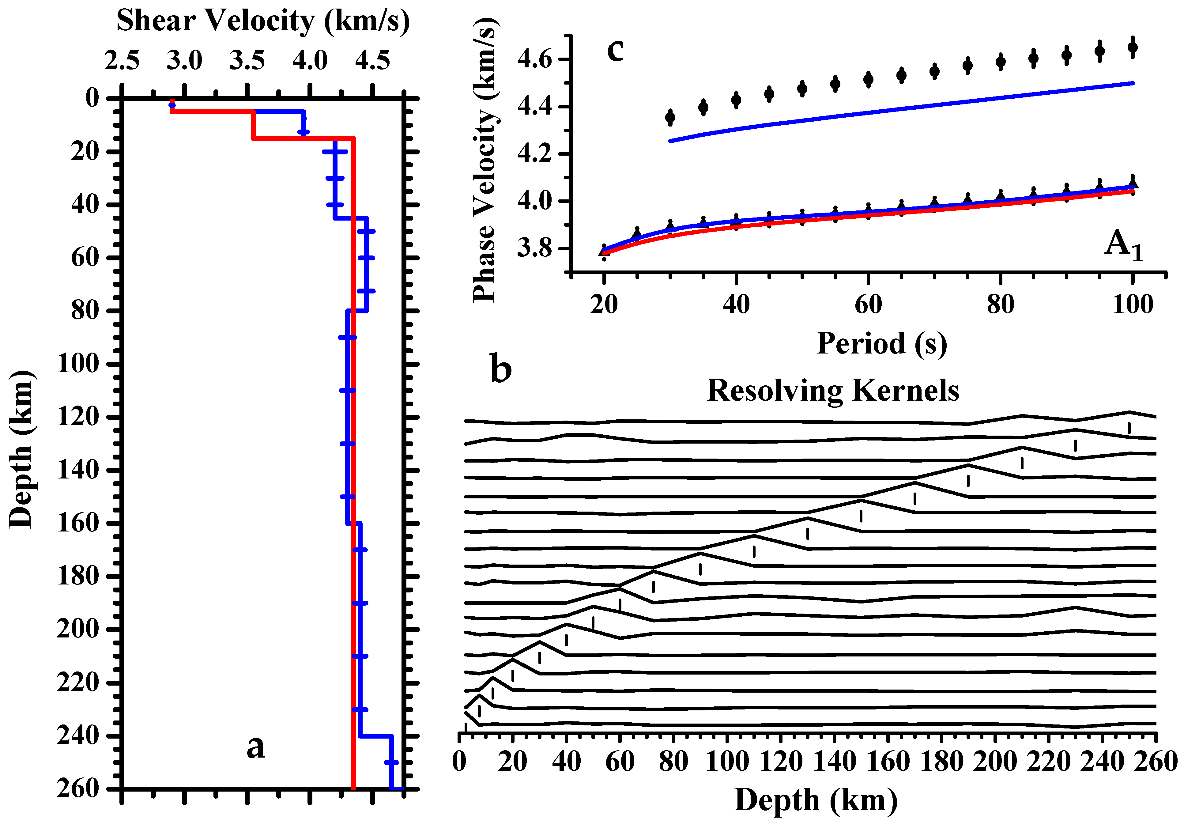
Period (s) | (degrees) | (km/s) | (degrees) | (km/s) |
|---|---|---|---|---|
| 30 | 160.00 | 4.42 | 69.09 | 4.29 |
| 35 | 163.63 | 4.46 | 73.63 | 4.33 |
| 40 | 163.63 | 4.49 | 73.63 | 4.37 |
| 45 | 163.63 | 4.52 | 73.63 | 4.41 |
| 50 | 163.63 | 4.54 | 73.63 | 4.42 |
| 55 | 163.63 | 4.57 | 73.63 | 4.43 |
| 60 | 163.63 | 4.59 | 73.63 | 4.44 |
| 65 | 163.63 | 4.61 | 73.63 | 4.46 |
| 70 | 163.63 | 4.63 | 73.63 | 4.47 |
| 75 | 163.63 | 4.64 | 73.63 | 4.50 |
| 80 | 163.63 | 4.66 | 73.63 | 4.52 |
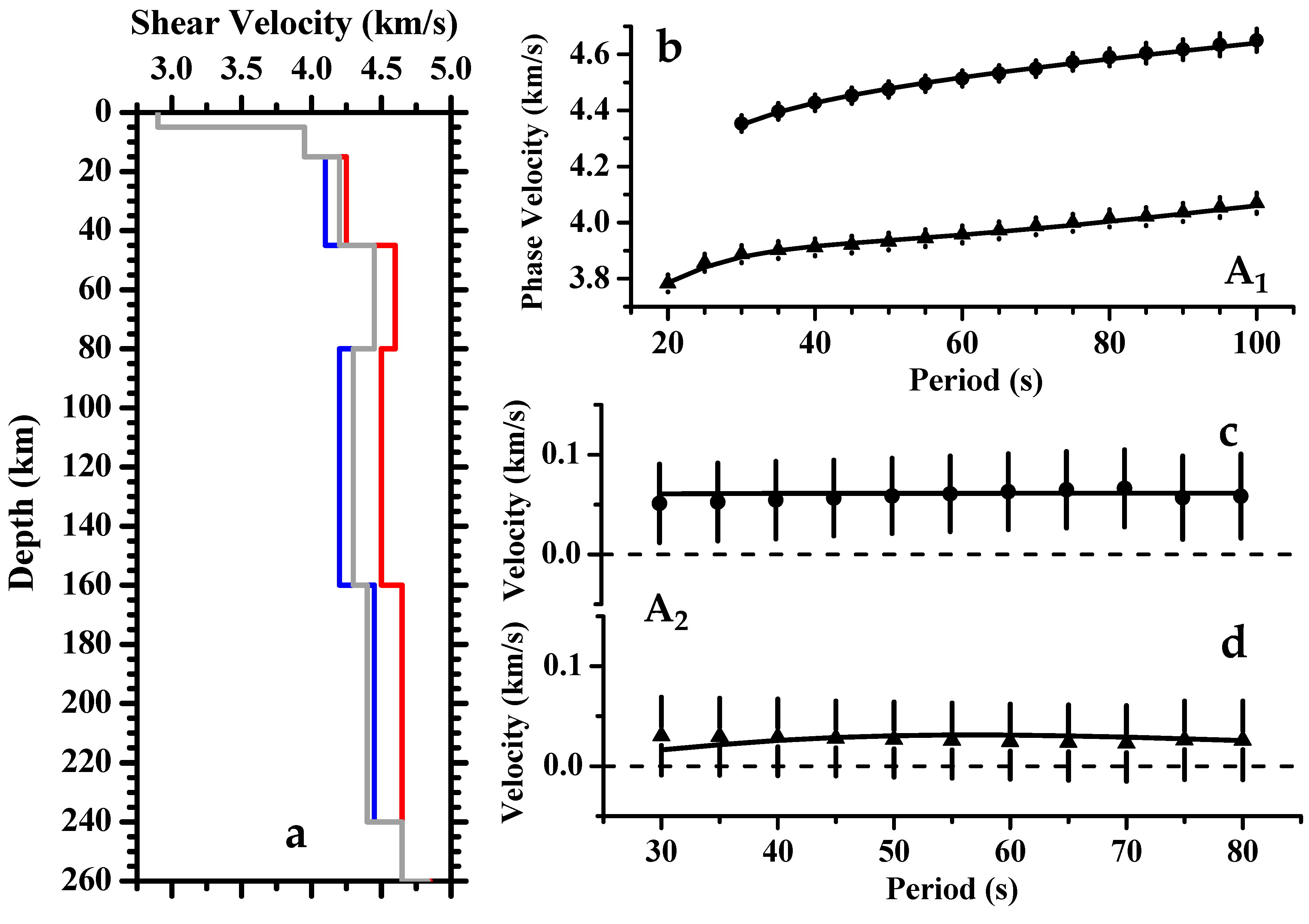
| Layer (n) | βH (km/s) | βV (km/s) | ξ (βH/βV)2 |
|---|---|---|---|
| 4 | 4.25 ± 0.07 | 4.11 ± 0.06 | 1.07 |
| 5 | 4.59 ± 0.08 | 4.45 ± 0.08 | 1.06 |
| 6 | 4.49 ± 0.08 | 4.21 ± 0.07 | 1.14 |
| 7 | 4.65 ± 0.08 | 4.44 ± 0.08 | 1.10 |
Disclaimer/Publisher’s Note: The statements, opinions and data contained in all publications are solely those of the individual author(s) and contributor(s) and not of MDPI and/or the editor(s). MDPI and/or the editor(s) disclaim responsibility for any injury to people or property resulting from any ideas, methods, instructions or products referred to in the content. |
© 2025 by the author. Licensee MDPI, Basel, Switzerland. This article is an open access article distributed under the terms and conditions of the Creative Commons Attribution (CC BY) license (https://creativecommons.org/licenses/by/4.0/).
Share and Cite
Corchete, V. Azimuthal Variation in the Surface Wave Velocity of the Philippine Sea Plate. J. Mar. Sci. Eng. 2025, 13, 606. https://doi.org/10.3390/jmse13030606
Corchete V. Azimuthal Variation in the Surface Wave Velocity of the Philippine Sea Plate. Journal of Marine Science and Engineering. 2025; 13(3):606. https://doi.org/10.3390/jmse13030606
Chicago/Turabian StyleCorchete, Víctor. 2025. "Azimuthal Variation in the Surface Wave Velocity of the Philippine Sea Plate" Journal of Marine Science and Engineering 13, no. 3: 606. https://doi.org/10.3390/jmse13030606
APA StyleCorchete, V. (2025). Azimuthal Variation in the Surface Wave Velocity of the Philippine Sea Plate. Journal of Marine Science and Engineering, 13(3), 606. https://doi.org/10.3390/jmse13030606