
Extreme Short-Term Prediction of Unmanned Surface Vessel Nonlinear Motion Under Waves


Abstract
:1. Introduction
2. Methodology
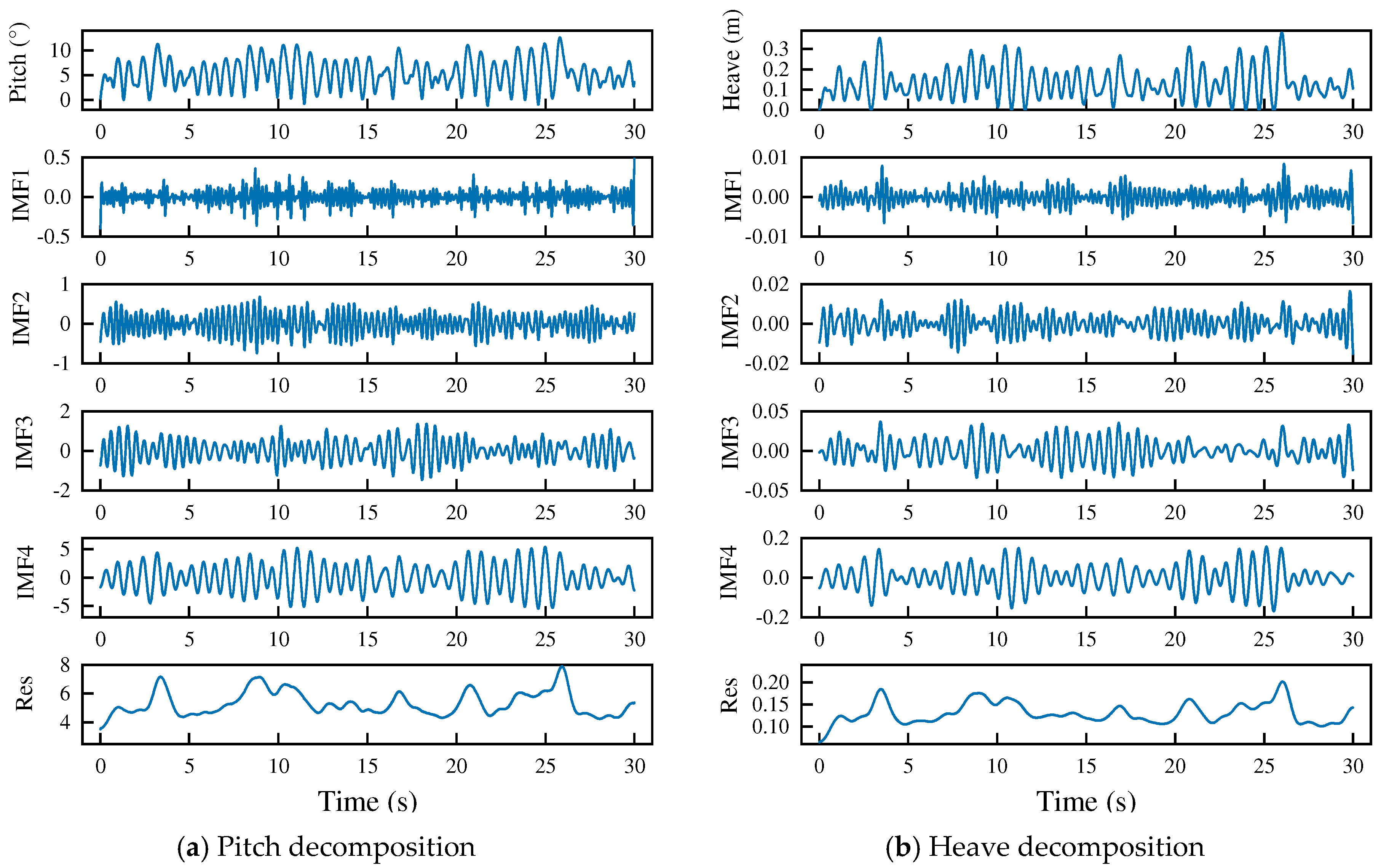
2.1. Variational Mode Decomposition (VMD)
2.2. Convolutional Neural Network (CNN)
2.3. Long Short-Term Memory (LSTM)
2.4. Evaluation Criterion
3. Data Source
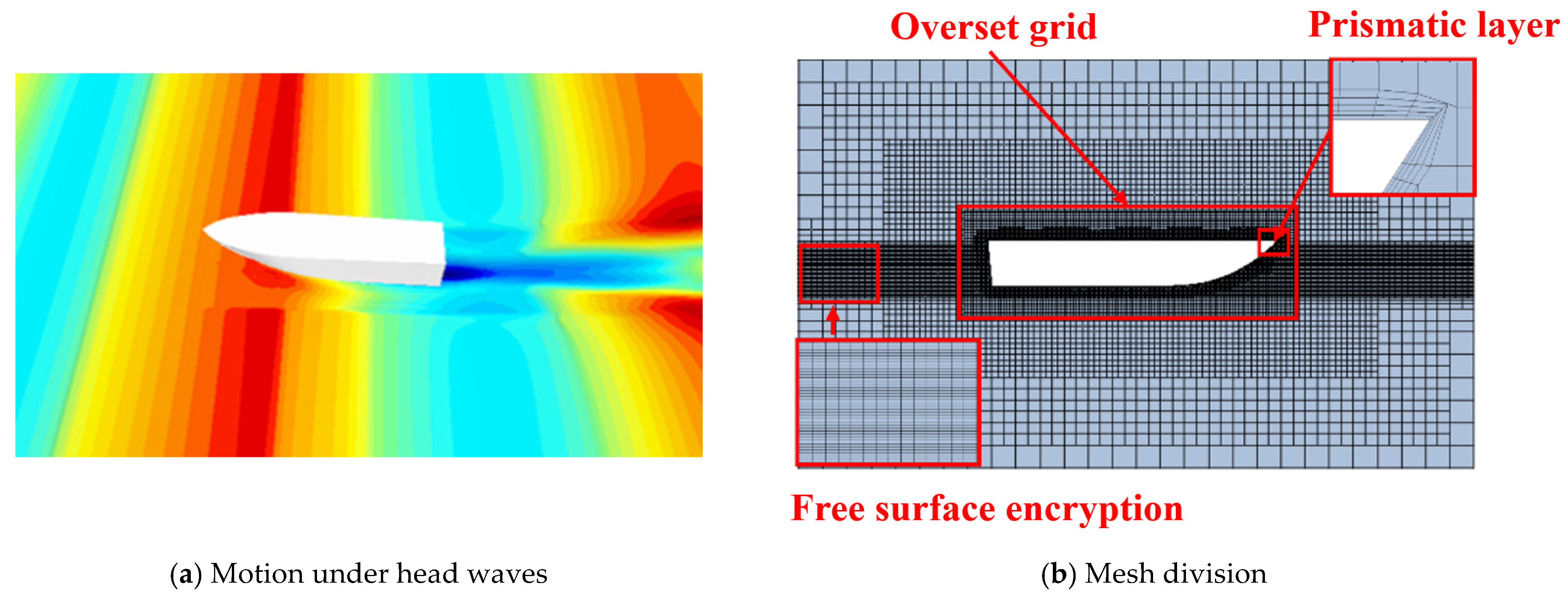
3.1. Validation of the Numerical Simulation Method
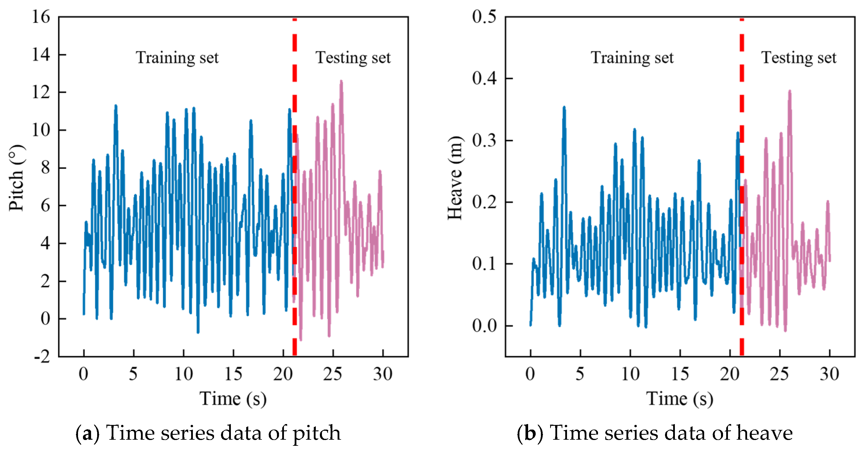
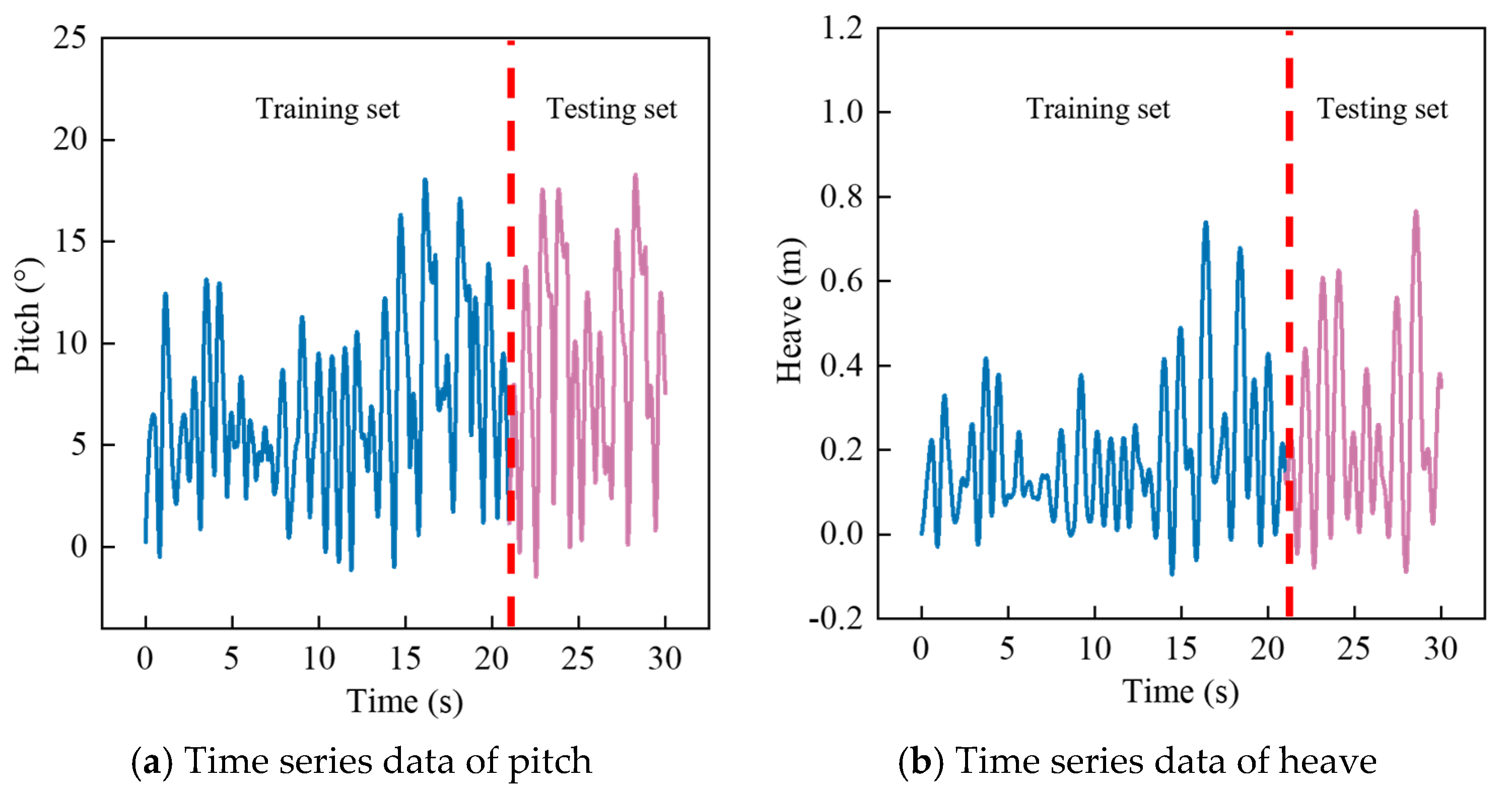
3.2. Dataset Generation
4. Prediction Results and Analysis of Nonlinear Motion Response of the USV
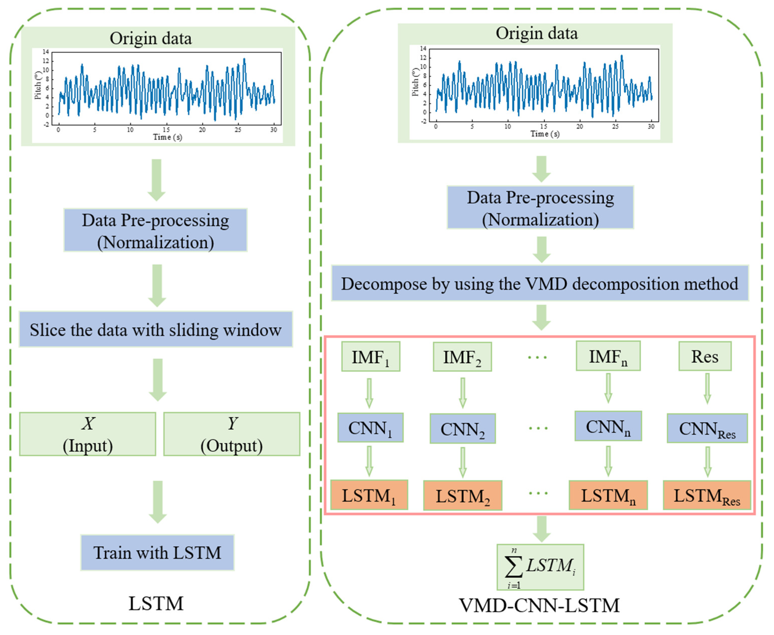
4.1. The Proposed VMD-CNN-LSTM Model
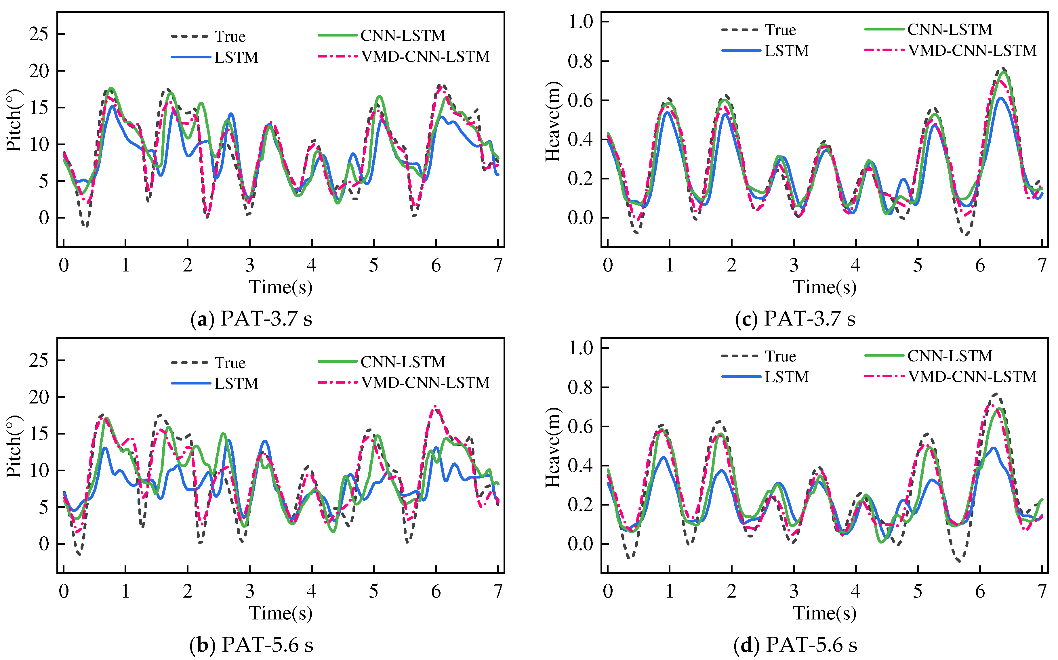
4.2. Performance Analysis
5. Conclusions
Author Contributions
Funding
Data Availability Statement
Conflicts of Interest
References
- Yang, P.; Xue, J.; Hu, H. A bibliometric analysis and overall review of the new technology and development of Unmanned Surface Vessels. J. Mar. Sci. Eng. 2024, 12, 146. [Google Scholar] [CrossRef]
- Yang, T.; Sun, N.; Chen, H.; Fang, Y. Neural network-based adaptive antiswing control of an underactuated ship-mounted crane with roll motions and input dead zones. IEEE Trans. Neural Netw. Learn. Syst. 2019, 31, 901–914. [Google Scholar] [CrossRef]
- Zhang, M.; Hao, S.; Wu, D.; Wu, D.; Yuan, Z. Time-optimal obstacle avoidance of autonomous ship based on nonlinear model predictive control. Ocean Eng. 2022, 266, 112591. [Google Scholar] [CrossRef]
- Ma, C.; Zhang, X.; Yang, G.P. Improved nonlinear control for ship course-keeping based on Lyapunov stability. Chin. J. Ship Res. 2019, 14, 150–155+161. [Google Scholar]
- Fossen, T.I.; Perez, T. Kalman filtering for positioning and heading control of ships and offshore rigs. Control Syst. IEEE 2009, 29, 32–46. [Google Scholar]
- Jiang, H.; Duan, S.; Huang, L.; Han, Y.; Ma, Q. Scale effects in AR model real-time ship motion prediction. Ocean Eng. 2020, 203, 107202. [Google Scholar] [CrossRef]
- John, J.S.; Arunachalam, V.; Coronado, F.K.; Romero, O.L.; Ramirez, Y.Y. Time-series modeling of fishery landings in the Colombian Pacific Ocean using an ARIMA model. Reg. Stud. Mar. Sci. 2020, 39, 101477. [Google Scholar]
- Huang, L.; Duan, W.; Han, Y.; Chen, Y. A review of short-term prediction techniques for ship motions in seaway. J. Ship Mech. 2014, 18, 1534–1542. [Google Scholar]
- Zhou, H.; Chen, Y.; Zhang, S. Ship trajectory prediction based on BP neural network. J. Artif. Intell. 2019, 1, 29–36. [Google Scholar] [CrossRef]
- Duan, S.; Ma, Q.; Huang, L.; Ma, X. A LSTM deep learning model for deterministic ship motions estimation using wave-excitation inputs. In Proceedings of the 29th International Ocean and Polar Engineering Conference, Honolulu, HI, USA, 16–21 June 2019. [Google Scholar]
- Duan, W.; Huang, L.; Han, Y. A hybrid AR-EMD-SVR model for the short-term prediction of nonlinear and non-stationary ship motion. J. Zhejiang Univ. Sci. A 2015, 16, 562–576. [Google Scholar] [CrossRef]
- Wang, W.; Li, M. A Short-time Prediction Method of Ship Motion Attitude Based on EEMD-LSSVM. Int. J. Sci. 2020, 7, 66–74. [Google Scholar]
- Khan, A.; Bil, C.; Marion, K.; Crozier, M. Real time prediction of ship motions and attitudes using advantage prediction techniques. In Proceedings of the 24th International Congress of the Aeronautical Sciences, Yokohama, Japan, 29 August–3 September 2004. [Google Scholar]
- Hochreiter, S.; Schmidhuber, J. Long Short-Term Memory. Neural Comput. 1997, 9, 1735–1780. [Google Scholar] [CrossRef] [PubMed]
- Chong, Y.; Xiong, H. A prediction method of ship motion based on LSTM neural network with variable step-variable sampling frequency characteristics. J. Mar. Sci. Eng. 2023, 11, 919. [Google Scholar] [CrossRef]
- Zhang, D.; Zhou, X.; Wang, Z.; Yan, P.; Xie, S. A data driven method for multi-step prediction of ship roll motion in high sea states. Ocean Eng. 2023, 276, 114230. [Google Scholar] [CrossRef]
- Wang, Y.; Wang, H.; Zhou, B.; Fu, H. Multi-dimensional prediction method based on Bi-LSTMC for ship roll. Ocean Eng. 2021, 242, 110106. [Google Scholar] [CrossRef]
- Dong, L.; Ma, X.; Feng, J.; Kong, L.; Liu, Y.; Wang, H. Online prediction method of ship maneuvering motion based on improved long-short term memory neural network. Shipbuild. China 2023, 64, 184–198. [Google Scholar]
- Zhan, K.; Zhu, R. A CNN-LSTM ship motion extreme value prediction model. J. Shanghai Jiao Tong Univ. 2023, 57, 963–971. [Google Scholar]
- Zhang, B.; Peng, X.; Gao, J. Ship motion attitude prediction based on ELM-EMD-LSTM integrated model. J. Ship Mech. 2020, 24, 1413–1421. [Google Scholar]
- Zuo, S.; Zhao, Q.; Zhang, B.; Pang, M.; Zhou, M. Prediction of ship motion attitude based on VMD-SSA-GRU model. Ship Sci. Technol. 2022, 44, 60–65. [Google Scholar]
- Gong, X.; Datla, R.J.; Xiang, X. Seakeeping evaluation of a Tri-SWACH based on CFD calculations and model tests. In Proceedings of the SNAME 26th Offshore Symposium, Virtual, 6–7 April 2021. [Google Scholar]
- Wang, X.; Sun, S.; Zhao, X. Research on model test of thousands-tons class high seakeeping performance hybrid monohull. J. Ship Mech. 2011, 15, 342–349. [Google Scholar]
- Wu, Q.; Zhang, B. Calculation methods of added resistance and ship motion response based on potential flow and viscous flow theory. China Ocean Eng. 2022, 36, 488–499. [Google Scholar] [CrossRef]
- Yu, L.; Wu, S.; Gu, Z.; Wu, C.; Li, C. Research on ship motion characteristics in a cross sea based on computational fluid dynamics and potential flow theory. Eng. Appl. Comput. Fluid Mech. 2023, 17, 2164618. [Google Scholar]
- Lee, E.J.; Schleicher, C.C.; Merrill, C.F.; Fullerton, A.M.; Geiser, J.S.; Weil, C.R.; Morin, J.R.; Jiang, J.; Stern, F.; Mousaviraad, S.M.; et al. Benchmark testing of Generic Prismatic Planing Hull (GPPH) for validation of CFD tools. In Proceedings of the SNAME 30th American Towing Tank Conference, West Bethesda, MD, USA, 4 October 2017. [Google Scholar]
- Li, J. Verification and Validation Study of OpenFOAM on the Generic Prismatic Planing Hull Form. Master’s Thesis, Virginia Polytechnic Institute and State University, Blacksburg, VA, USA, 2019. [Google Scholar]
- Dragomiretskiyk, K.; Zosso, D. Variational Mode Decomposition. IEEE Trans. Signal Process. 2014, 62, 531–544. [Google Scholar] [CrossRef]
- Diez, M.; Lee, E.J.; Harrison, E.L.; Stern, F. Experimental and computational fluid-structure interaction analysis and optimization of deep-V planning-hull grillage panels subject to slamming loads—Part I: Regular waves. Mar. Struct. 2022, 85, 103256. [Google Scholar] [CrossRef]
- Lee, E.J.; Diez, M.; Harrison, E.L.; Jiang, J.; Snyder, L.A.; Powres, A.R.; Bay, R.J.; Serani, A.; Nadal, M.L.; Kubina, E.R.; et al. Experimental and computational fluid-structure interaction analysis and optimization of deep-V planning-hull grillage panels subject to slamming loads—Part II: Irregular waves. Ocean Eng. 2024, 292, 116346. [Google Scholar] [CrossRef]
- ITTC. ITTC Quality System Manual Recommended Procedures and Guidelines: Practical Guidelines for Ship CFD Application. In Proceedings of the 27th International Towing Tank Conference, Copenhagen, Denmark, 31 August–5 September 2014. [Google Scholar]
- Deng, S.; Ning, D.; Mayon, R. The motion forecasting study of floating offshore wind turbine using self-attention long short-term memory method. Ocean Eng. 2024, 310, 118709. [Google Scholar] [CrossRef]
- Shi, W.; Hu, L.; Lin, Z.; Zhang, L.; Wu, J.; Chai, W. Short-term motion prediction of floating offshore wind turbine based on muti-input LSTM neural network. Ocean Eng. 2023, 280, 114558. [Google Scholar] [CrossRef]


| Parameter | Units | Full Scale | Model Scale (λ = 5.4) |
|---|---|---|---|
| Overall length | m | 13.036 | 2.414 |
| Breadth | m | 4.001 | 0.741 |
| Displacement | kg | 15,000.984 | 101.510 |
| Draft | m | 0.788 | 0.146 |
| Longitudinal center of gravity | m | 4.644 | 0.860 |
| Vertical center of gravity | m | 0.745 | 0.138 |
| Pitch radius of gyration | m | 2.452 | 0.454 |
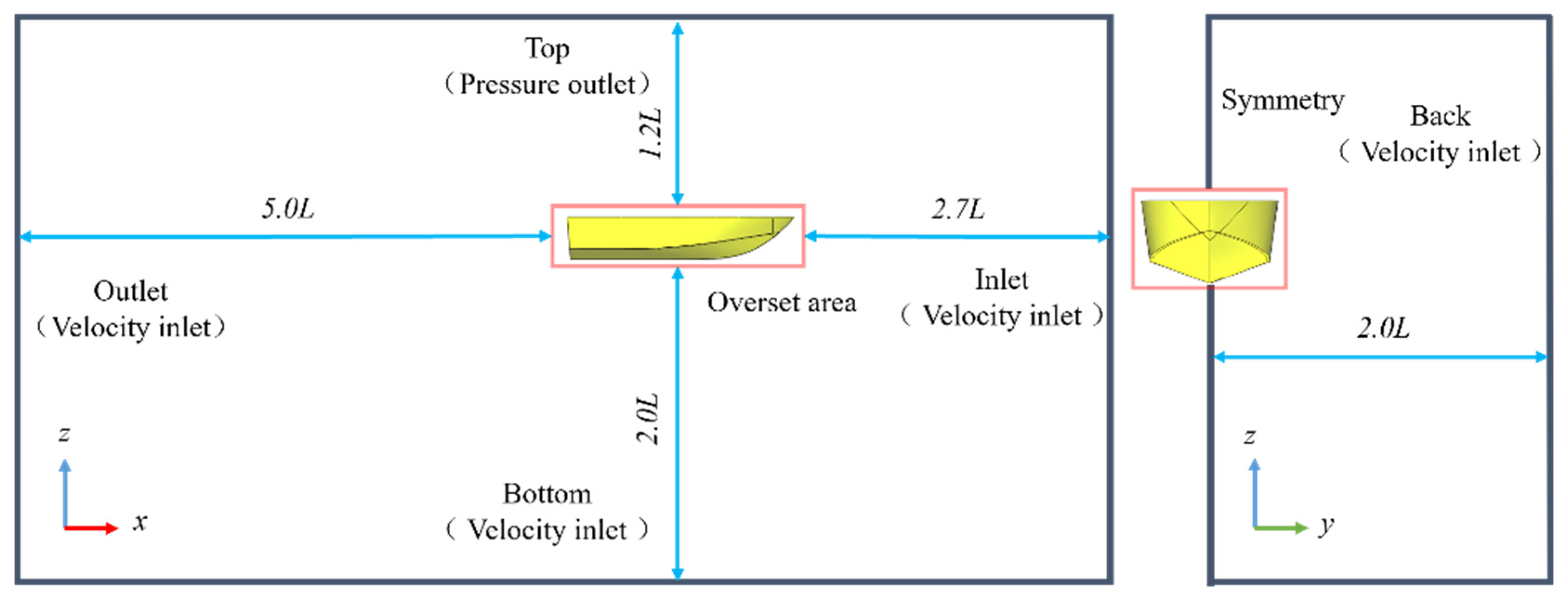
| Domain Type | Boundary | Boundary Condition |
|---|---|---|
| Background domain | Inlet | Velocity inlet |
| Outlet | Velocity inlet | |
| Back | Velocity inlet | |
| Symmetry | Symmetry plane | |
| Bottom | Velocity inlet | |
| Top | Pressure outlet | |
| Overset domain | Hull surface | Wall |
| Vertical boundary | Overset mesh | |
| Symmetry | Symmetry plane |
| Case | Hs (m) | Tp (s) |
|---|---|---|
| Case I | 1.015 | 5.577 |
| Case II | 1.998 | 6.507 |
| Parameters | Value |
|---|---|
| Max epochs | 150 |
| Initial learn rate | 0.01 |
| Loss function | Root Mean Squared Error |
| Optimizer | Adam |
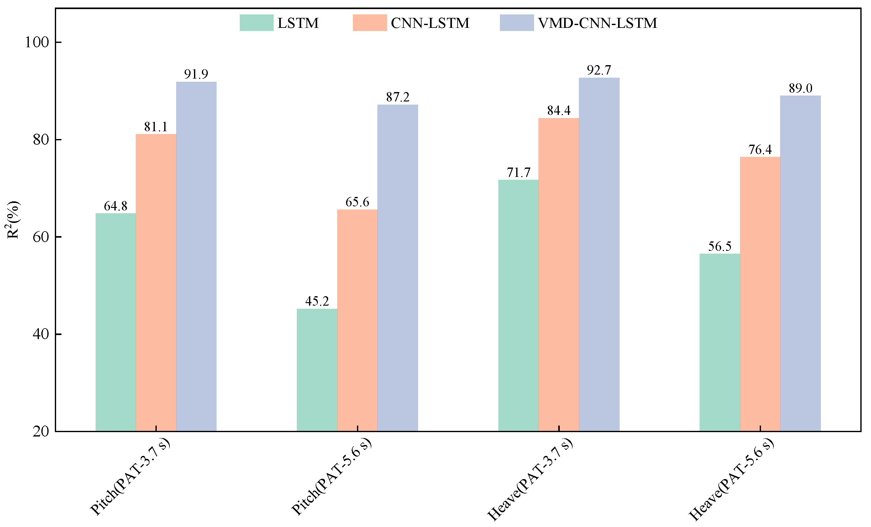
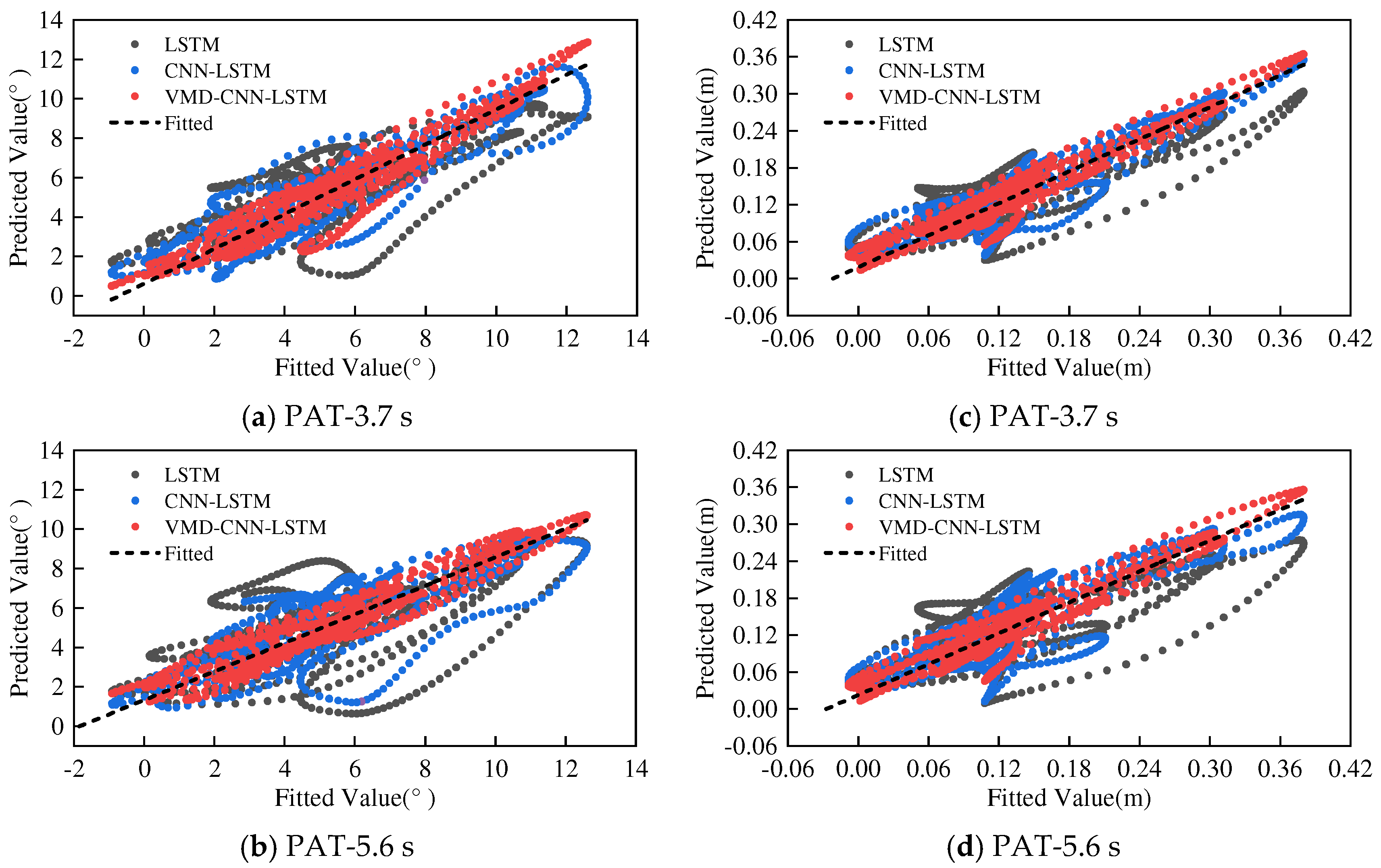
| Dataset | PAT (s) | Model | MSE | RMSE | MAE | R2 |
|---|---|---|---|---|---|---|
| Pitch (°) | 3.7 | LSTM | 2.968 | 1.723 | 1.418 | 0.648 |
| CNN-LSTM | 1.590 | 1.261 | 0.993 | 0.811 | ||
| VMD-CNN-LSTM | 0.678 | 0.824 | 0.639 | 0.919 | ||
| 5.6 | LSTM | 4.672 | 2.161 | 1.720 | 0.452 | |
| CNN-LSTM | 2.934 | 1.713 | 1.409 | 0.656 | ||
| VMD-CNN-LSTM | 1.097 | 1.048 | 0.834 | 0.872 | ||
| Heave (m) | 3.7 | LSTM | 0.002 | 0.045 | 0.036 | 0.711 |
| CNN-LSTM | 0.001 | 0.033 | 0.026 | 0.844 | ||
| VMD-CNN-LSTM | 0.0005 | 0.022 | 0.019 | 0.927 | ||
| 5.6 | LSTM | 0.003 | 0.055 | 0.044 | 0.565 | |
| CNN-LSTM | 0.002 | 0.041 | 0.032 | 0.764 | ||
| VMD-CNN-LSTM | 0.0007 | 0.027 | 0.021 | 0.890 |
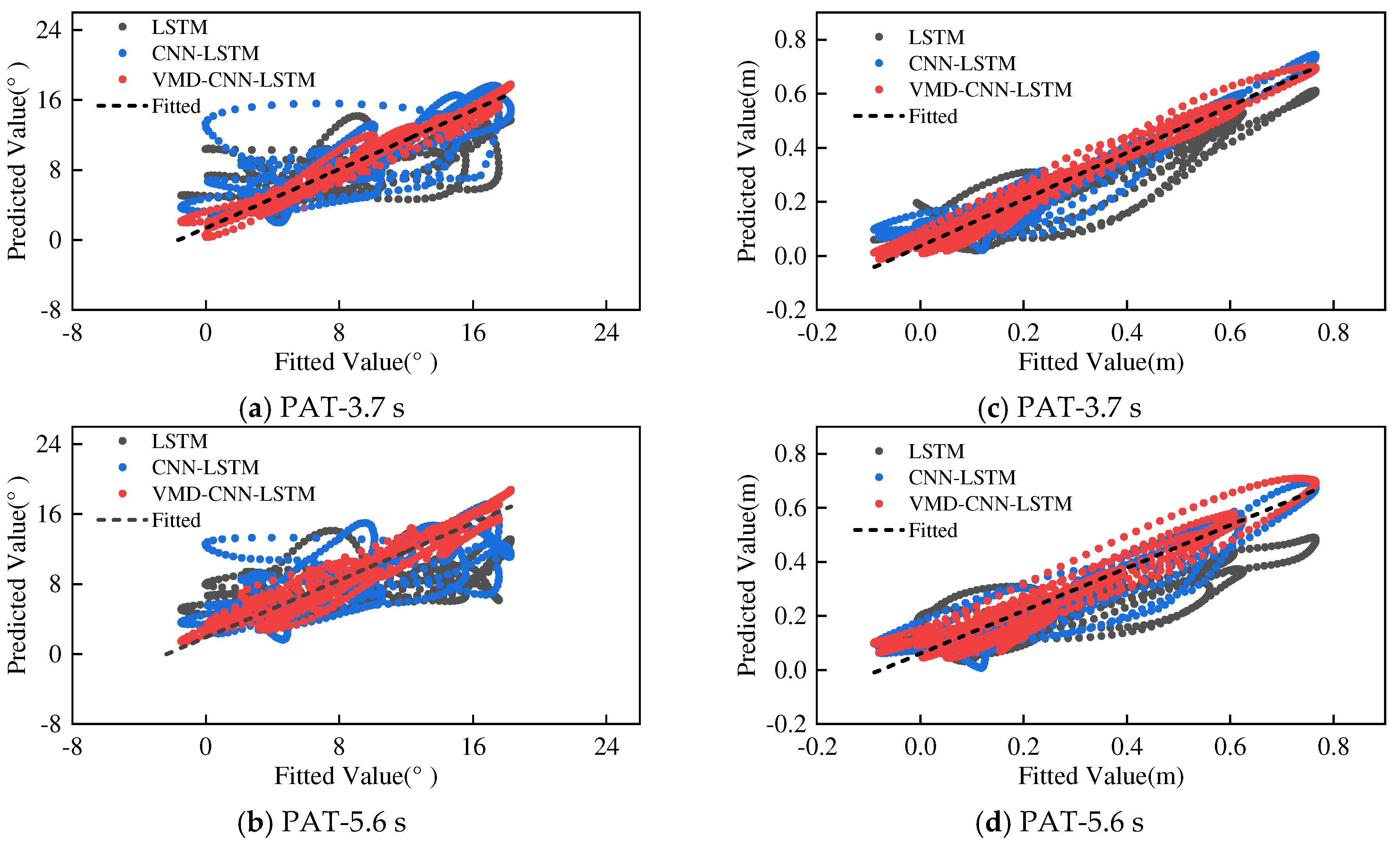
| Dataset | PAT (s) | Model | MSE | RMSE | MAE | R2 |
|---|---|---|---|---|---|---|
| Pitch (°) | 3.7 | LSTM | 14.952 | 3.867 | 3.058 | 0.410 |
| CNN-LSTM | 9.788 | 3.128 | 2.231 | 0.610 | ||
| VMD-CNN-LSTM | 1.383 | 1.176 | 0.944 | 0.945 | ||
| 5.6 | LSTM | 20.530 | 4.531 | 3.727 | 0.219 | |
| CNN-LSTM | 13.712 | 3.703 | 2.787 | 0.459 | ||
| VMD-CNN-LSTM | 2.712 | 1.647 | 1.321 | 0.893 | ||
| Heave (m) | 3.7 | LSTM | 0.010 | 0.101 | 0.084 | 0.770 |
| CNN-LSTM | 0.005 | 0.067 | 0.051 | 0.897 | ||
| VMD-CNN-LSTM | 0.002 | 0.043 | 0.034 | 0.959 | ||
| 5.6 | LSTM | 0.019 | 0.137 | 0.108 | 0.583 | |
| CNN-LSTM | 0.008 | 0.089 | 0.071 | 0.820 | ||
| VMD-CNN-LSTM | 0.004 | 0.068 | 0.054 | 0.894 |
Disclaimer/Publisher’s Note: The statements, opinions and data contained in all publications are solely those of the individual author(s) and contributor(s) and not of MDPI and/or the editor(s). MDPI and/or the editor(s) disclaim responsibility for any injury to people or property resulting from any ideas, methods, instructions or products referred to in the content. |
© 2025 by the authors. Licensee MDPI, Basel, Switzerland. This article is an open access article distributed under the terms and conditions of the Creative Commons Attribution (CC BY) license (https://creativecommons.org/licenses/by/4.0/).
Share and Cite
Wang, Y.; Li, J.; Wang, S.; Zhang, H.; Yang, L.; Wu, W. Extreme Short-Term Prediction of Unmanned Surface Vessel Nonlinear Motion Under Waves. J. Mar. Sci. Eng. 2025, 13, 610. https://doi.org/10.3390/jmse13030610
Wang Y, Li J, Wang S, Zhang H, Yang L, Wu W. Extreme Short-Term Prediction of Unmanned Surface Vessel Nonlinear Motion Under Waves. Journal of Marine Science and Engineering. 2025; 13(3):610. https://doi.org/10.3390/jmse13030610
Chicago/Turabian StyleWang, Yiwen, Jian Li, Shan Wang, Hantao Zhang, Long Yang, and Weiguo Wu. 2025. "Extreme Short-Term Prediction of Unmanned Surface Vessel Nonlinear Motion Under Waves" Journal of Marine Science and Engineering 13, no. 3: 610. https://doi.org/10.3390/jmse13030610
APA StyleWang, Y., Li, J., Wang, S., Zhang, H., Yang, L., & Wu, W. (2025). Extreme Short-Term Prediction of Unmanned Surface Vessel Nonlinear Motion Under Waves. Journal of Marine Science and Engineering, 13(3), 610. https://doi.org/10.3390/jmse13030610