
AGV Scheduling and Energy Consumption Optimization in Automated Container Terminals Based on Variable Neighborhood Search Algorithm


Abstract
:1. Introduction
2. Literature Review
3. Problem Description
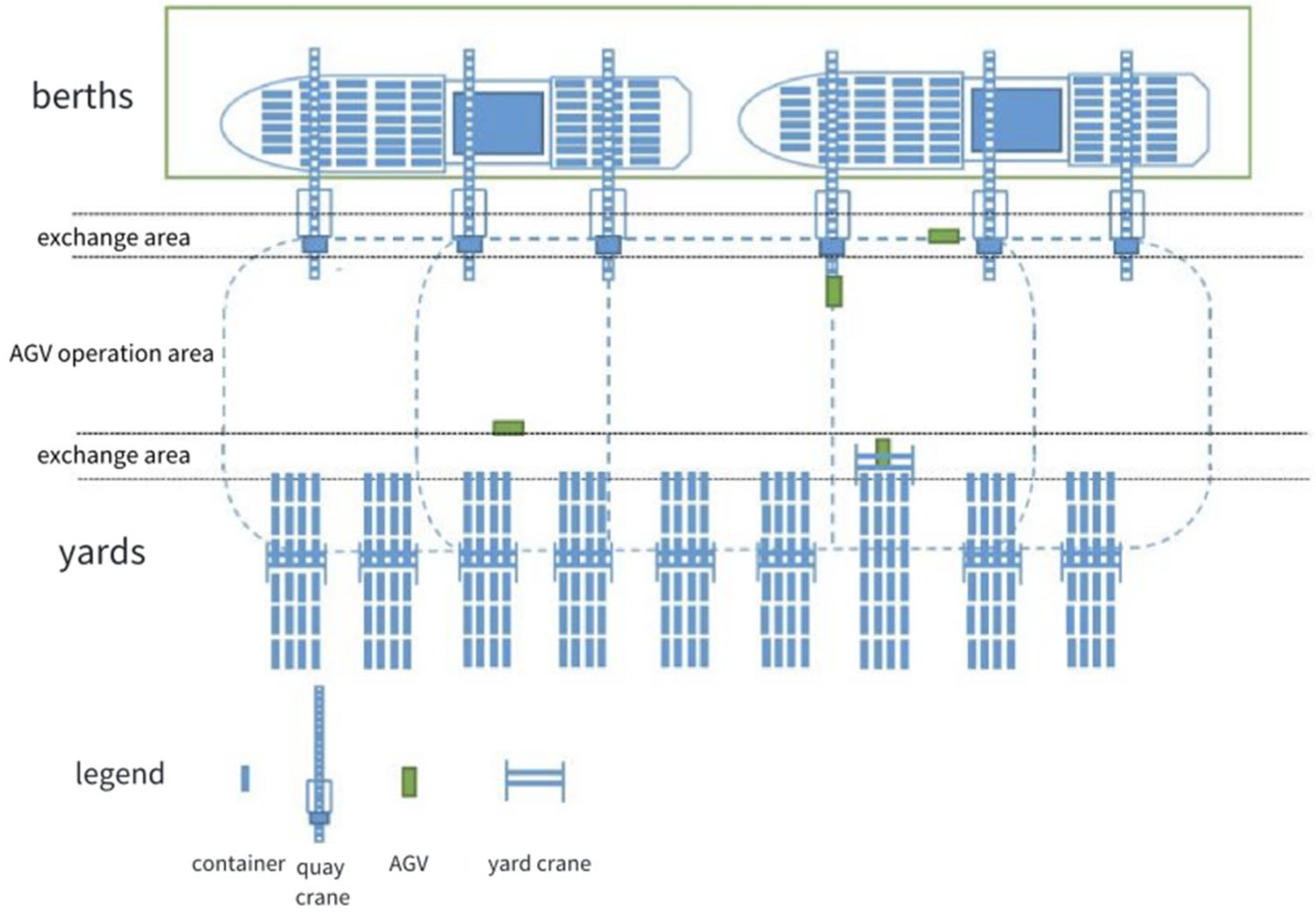
3.1. Horizontal Transportation Equipment Operation System
3.2. Horizontal Transportation Equipment
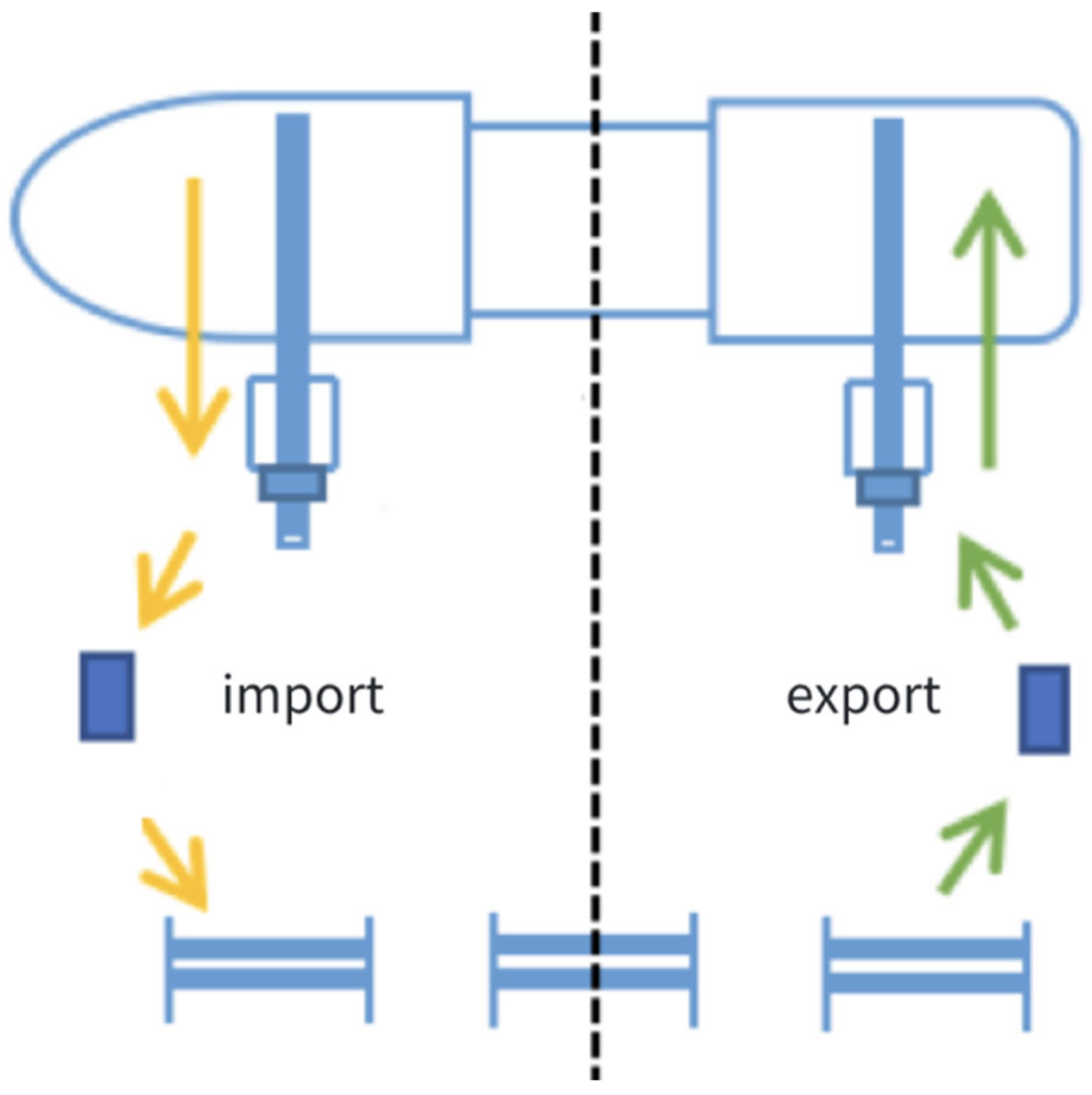
3.3. Energy Consumption and Scheduling of AGV
- Unloading to pick-up point: the AGV drives from the charging station (if the current task is the first task of the AGV) or the last task drop point to the current task pick-up point in the unloading state.
- Arrive at the pick-up point: After the AGV arrives at the designated yard or quay crane, it will judge whether it needs to wait by comparing the time axis of the AGV with the time axis of the yard or quay crane. If it needs to wait, the AGV will generate the waiting cost until the yard or quay crane completes the last container operation; if it does not need to wait, it will directly proceed to the next operation.
- AGV operation: The AGV waits for the yard or quay crane to load the container onto it (the waiting time depends on the loading operation time). Then, the AGV goes to the drop point of the current container in the loading state.
- Arrive at the drop point: After the AGV arrives at the designated quay or yard crane, it will judge whether it needs to wait again by comparing the time axis of the AGV with the time axis of the quay or yard crane. If it needs to wait, the AGV will generate the waiting cost until the quay or yard crane completes the last container operation; if it does not need to wait, it will directly proceed to the next operation.
- Unloading operation: The AGV waits for the quay or yard crane to unload the container from it. After that, the AGV can directly go to the next pick-up point without waiting for the quay or yard crane to store the current container in the container yard.
4. Modeling
4.1. Model Assumptions
- (1)
- An AGV has sufficient power during the entire operation process, and the charging process is not considered.
- (2)
- Traffic problems such as congestion and AGV path planning are not considered.
- (3)
- An AGV only transports one container at a time.
- (4)
- An AGV drives at a constant speed throughout the entire operation process.
4.2. Model Parameter Settings
4.3. Decision Variables
4.4. Model Establishment
5. Variable Neighborhood Search Algorithm
5.1. The Introduction of Variable Neighborhood Search
5.2. Algorithm Design
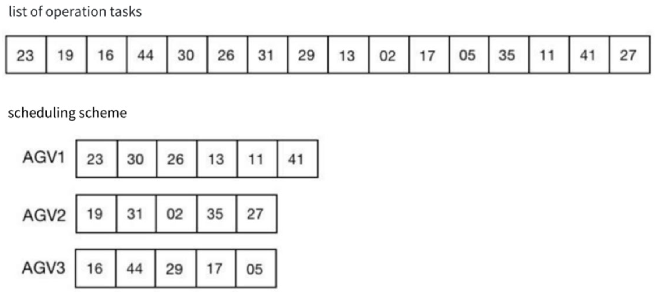
5.2.1. Coding
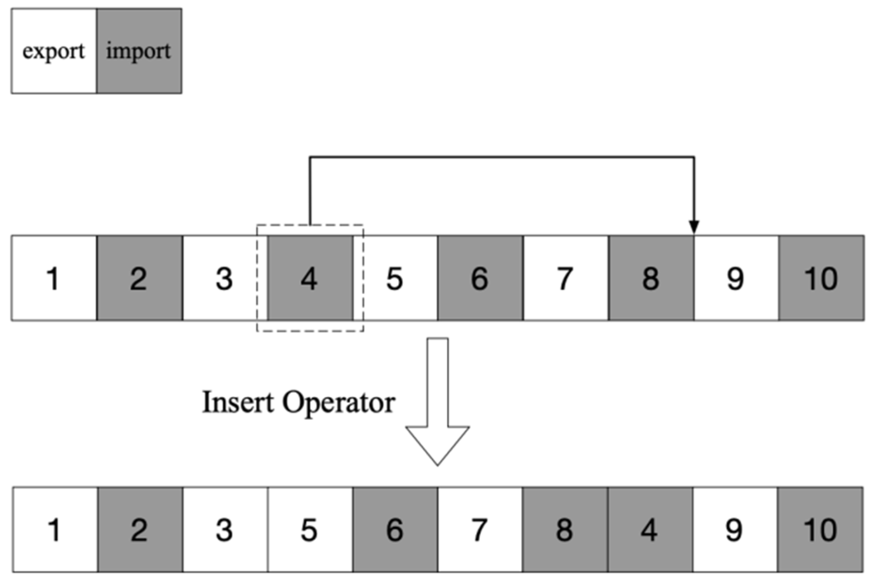
5.2.2. Operators
- (1)
- Insert Operator
- (2)
- Swap Operator
- (3)
- Reverse Operator
- (4)
- Block Swap Operator
- (5)
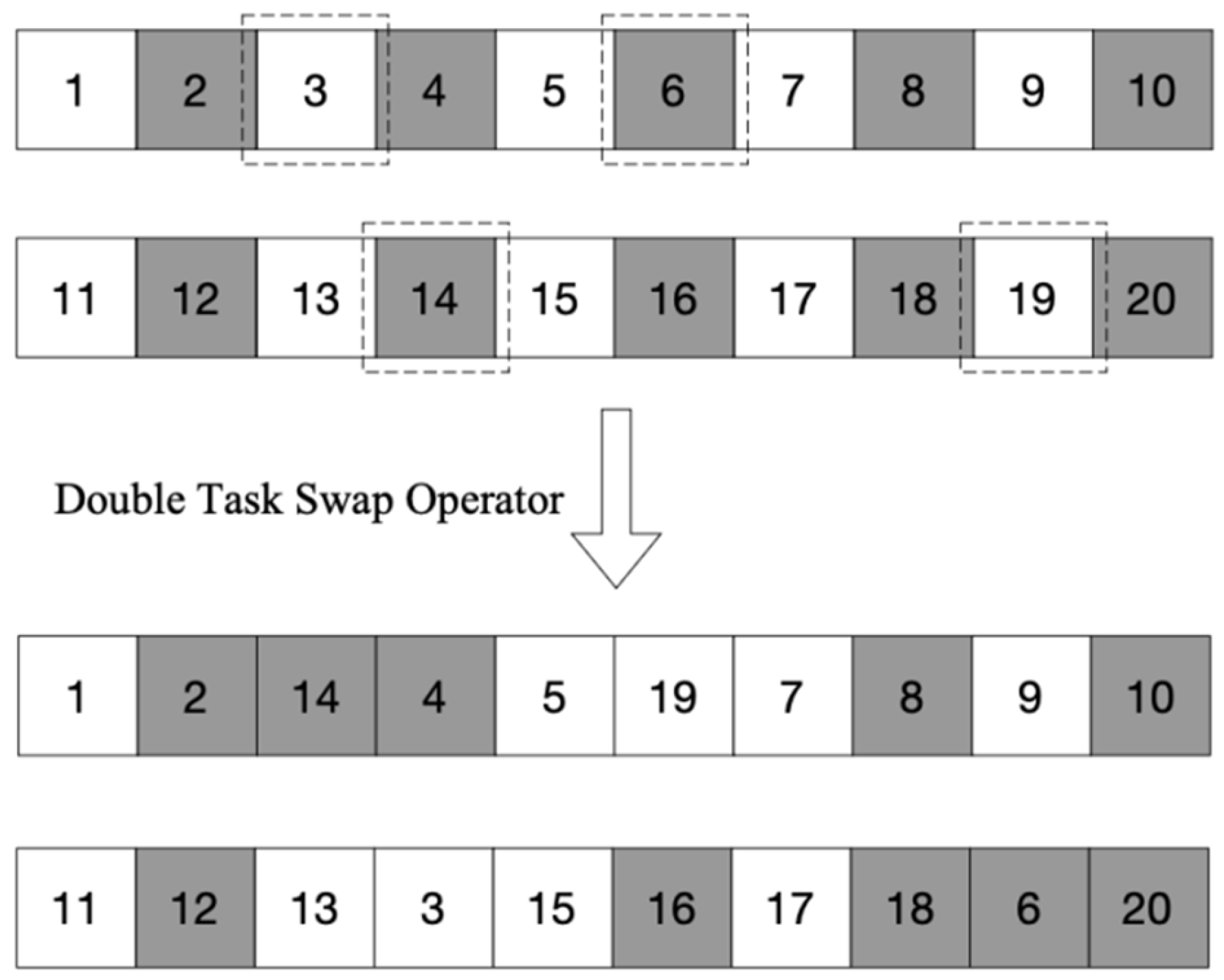
- Double Task Swap Operator
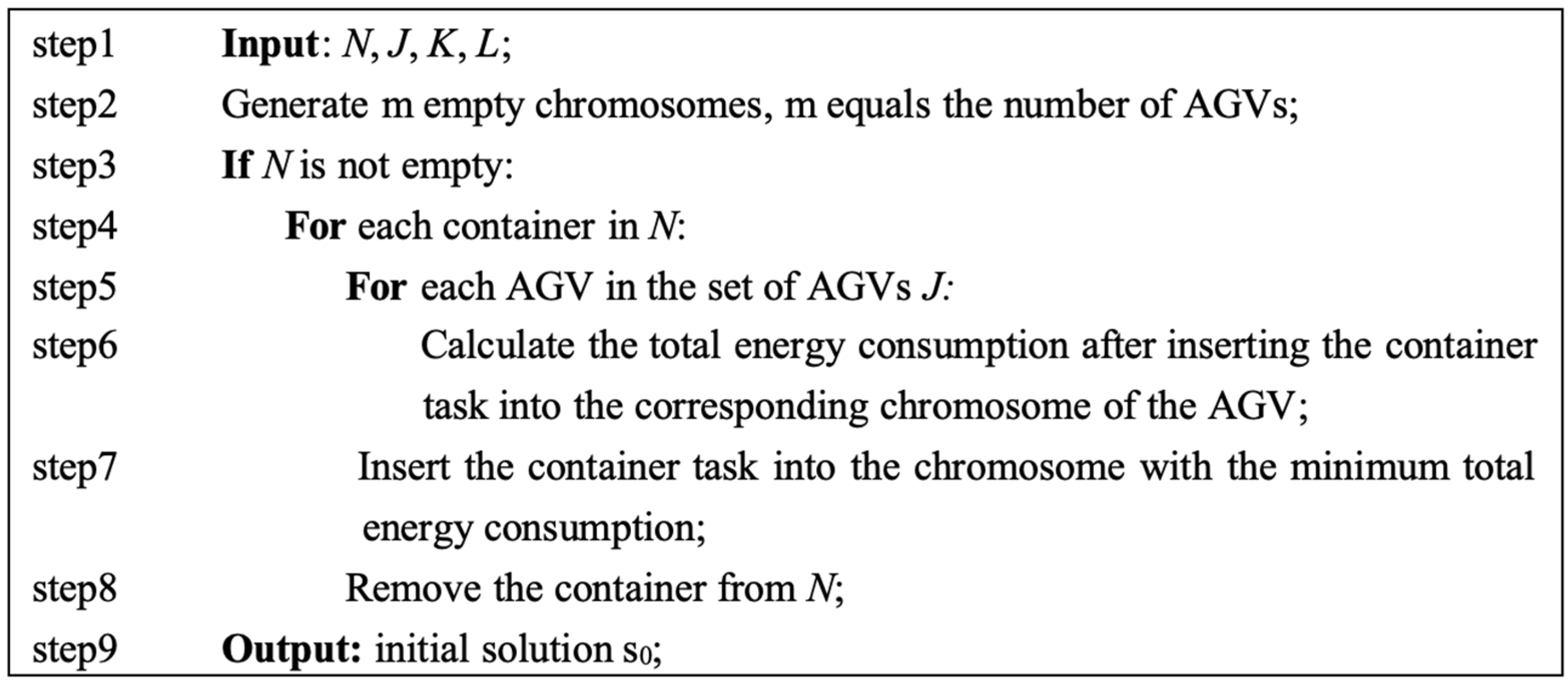
5.2.3. Initial Solution
5.2.4. Calculation of Objective Function
5.3. Process of Algorithmic Solution
6. Numerical Experiments
6.1. Example Design
6.2. Small-Scale Example
6.2.1. Comparison of the Number of AGVs in Small-Scale
6.2.2. Comparison of Algorithms in Small-Scale
6.2.3. Convergence Analysis in Small-Scale
6.3. Large-Scale Example
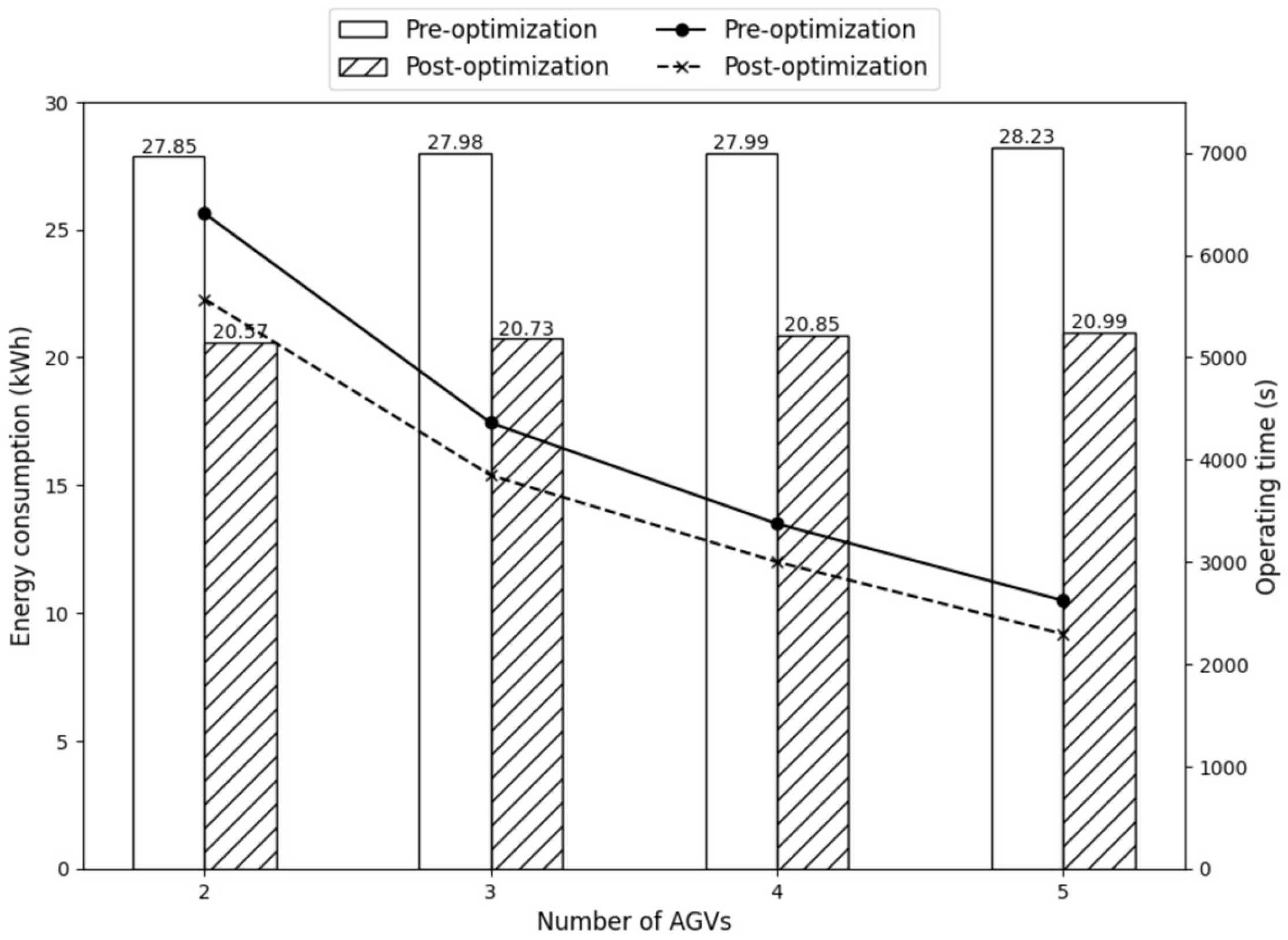
6.3.1. Comparison of the Number of AGVs in Large-Scale
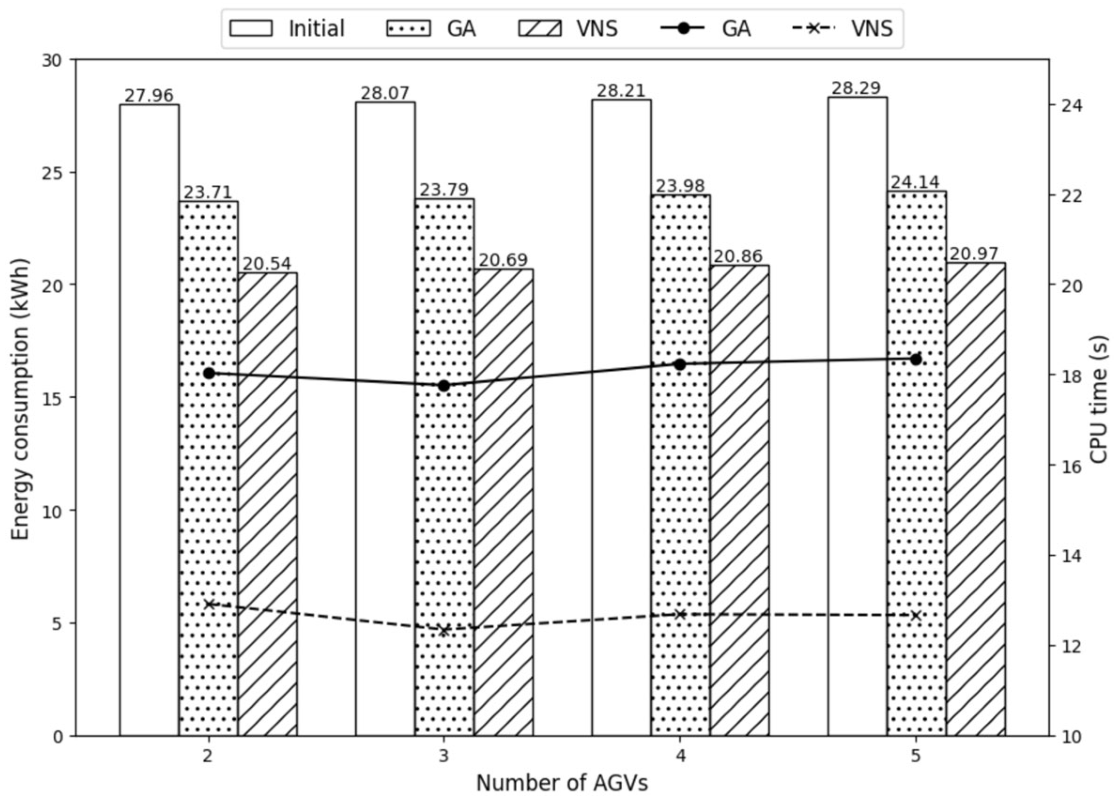
6.3.2. Comparison of Algorithms in Large-Scale
6.3.3. Convergence Analysis in Large-Scale
6.4. Analysis of AGV Speed Change
7. Conclusions
Author Contributions
Funding
Data Availability Statement
Conflicts of Interest
References
- Yue, L. Research on Configuration and Scheduling of Double-Trolley Quay Crane and AGV in Automated Container Terminal; Dalian Maritime University: Dalian, China, 2020. [Google Scholar]
- Wang, Z.; Hu, W. Cooperative scheduling of loading and unloading equipment in automated container terminal considering AGV path conflict. Ind. Eng. Manag. 2023, 28, 80–92. [Google Scholar]
- Bae, J.W.; Kim, K.H. A pooled dispatching strategy for automated guided vehicles in port container terminals. Manag. Sci. Financ. Eng. 2000, 6, 47–67. [Google Scholar]
- Zhao, Q.; Ji, S.; Guo, D.; Du, X.; Wang, H. Research on Cooperative Scheduling of Automated Quayside Cranes and Automatic Guided Vehicles in Automated Container Terminal. Math. Probl. Eng. 2019, 2019, 6574582. [Google Scholar]
- Yang, Y.; Zhong, M.; Dessouky, Y.; Postolache, O. An Integrated Scheduling Method for AGV Routing in Automated Container Terminals. Comput. Ind. Eng. 2018, 126, 482–493. [Google Scholar]
- Choe, R.; Kim, J.; Ryu, K.R. Online preference learning for adaptive dispatching of AGVs in an automated container terminal. Appl. Soft Comput. 2016, 38, 647–660. [Google Scholar] [CrossRef]
- Zhao, T.; Liang, C.J.; Hu, X.Y.; Wang, Y. Solution of AGV scheduling and battery exchange two-layer model for automated container terminal. J. Dalian Univ. Technol. 2021, 61, 623–633. [Google Scholar]
- Zeng, Q.; Li, M.; Yun, X. Modeling of AGV assignment considering charging factors at automated container terminals. Oper. Res. Manag. Sci. 2024, 33, 56–62. [Google Scholar]
- Xu, P.; Liang, C. Research on multi-AGV scheduling optimization of automated container terminal considering number of battery packs. Appl. Res. Comput. 2022, 39, 2653–2659. [Google Scholar]
- Ma, N.; Hu, Z. Congestion-aware AGV charging strategy in automated container terminal. Comput. Integr. Manuf. Syst. 2024, 30, 2621–2630. [Google Scholar]
- Drungilas, D.; Kurmis, M.; Senulis, A.; Lukosius, Z.; Andziulis, A.; Januteniene, J.; Bogdevicius, M.; Jankunas, V.; Voznak, M. Deep reinforcement learning based optimization of automated guided vehicle time and energy consumption in a container terminal. Alex. Eng. J. 2023, 67, 397–407. [Google Scholar] [CrossRef]
- Yang, X.; Hu, H.; Jin, J. Battery-powered automated guided vehicles scheduling problem in automated container terminals for minimizing energy consumption. Ocean Coast. Manag. 2023, 246, 106873. [Google Scholar] [CrossRef]
- Wang, C.; Jin, C.; Li, Z. Bilevel programming model of low energy consumption AGV scheduling problem at automated container terminal. In Proceedings of the 2019 IEEE International Conference on Smart Manufacturing, Industrial & Logistics Engineering, Hangzhou, China, 20–21 April 2019; IEEE: Piscataway, NJ, USA; pp. 195–199. [Google Scholar]
- Zhou, W.; Zhang, Y.; Tang, K.; He, L.; Zhang, C.; Tian, Y. Co-optimization of the operation and energy for AGVs considering battery-swapping in automated container terminals. Comput. Ind. Eng. 2024, 195, 110445. [Google Scholar]
- Yang, J.; Yu, F.; Wu, E.; Yang, Y. Energy saving of automated terminals considering AGV speed variation. In Proceedings of the 2022 International Symposium on Sensing and Instrumentation in 5G and IoT Era, ISSI 2022, Shanghai, China, 17–18 November 2022; pp. 68–73. [Google Scholar]
- Xing, Z.; Liu, H.; Wang, T.; Chew, E.P.; Lee, L.H.; Tan, K.C. Integrated automated guided vehicle dispatching and equipment scheduling with speed optimization. Transp. Res. Part E Logist. Transp. Rev. 2023, 169, 102993. [Google Scholar] [CrossRef]
- Chu, L.; Liang, D. Multiobjective scheduling optimization of AGVs in DQN algorithm-based automated container terminals. J. Harbin Eng. Univ. 2024, 45, 996–1004. [Google Scholar]
- Zhao, Q. Collaborative Scheduling Optimization of Operation Equipment in Automated Container Terminal Considering Energy Consumption; Beijing Jiaotong University: Beijing, China, 2021. [Google Scholar]
- Fan, H.; Guo, Z.; Yue, L.; Ma, M. Joint configuration and scheduling optimization of dual-trolley quay crane and AGV for container terminal with considering energy saving. Acta Autom. Sin. 2021, 47, 2412–2426. [Google Scholar]
- Ai, L.; Han, X. Coordinated scheduling of handling equipments at automated terminals considering energy consumption. J. Shanghai Marit. Univ. 2018, 39, 26–31. [Google Scholar]
- Yang, J.; Yu, F.; Yang, Y. Multi-Equipment coordinated scheduling considering energy consumption in sea-rail intermodal container terminal. Comput. Eng. 2024, 50, 393–404. [Google Scholar]


| Parameter | Description | Value |
|---|---|---|
| vf | Loading speed of AGV/(m/s) | 3.5 |
| ve | Unloading speed of AGV/(m/s) | 6 |
| Cf | Energy consumption of AGV in loading state/(kWh/s) | 0.006 |
| Ce | Energy consumption of AGV in unloading state/(kWh/s) | 0.004 |
| Cw | Energy consumption of AGV in waiting state/(kWh/s) | 0.0025 |
| Number of AGVs | Pre-Optimization | Post-Optimization | Decrease | |||
|---|---|---|---|---|---|---|
| EC (kWh) | OT (s) | EC (kWh) | OT (s) | EC | OT | |
| 2 | 27.85 | 6406.64 | 20.57 | 5568.61 | 26.14% | 13.09% |
| 3 | 27.98 | 4358.53 | 20.73 | 3845.59 | 25.91% | 11.77% |
| 4 | 27.99 | 3372.59 | 20.85 | 2999.17 | 25.51% | 11.07% |
| 5 | 28.23 | 2621.11 | 20.99 | 2294.20 | 25.65% | 12.47% |
| Number of AGVs | Initial EC (kWh) | GA [15] | VNS | Gap | |||||
|---|---|---|---|---|---|---|---|---|---|
| EC (kWh) | OR | CPU Time (s) | EC (kWh) | OR | CPU Time (s) | EC | CPU Time | ||
| 2 | 27.96 | 23.71 | 15.20% | 18.03 | 20.54 | 26.54% | 12.91 | 13.37% | 28.40% |
| 3 | 28.07 | 23.79 | 15.25% | 17.76 | 20.69 | 26.29% | 12.34 | 13.03% | 30.52% |
| 4 | 28.21 | 23.98 | 14.99% | 18.23 | 20.86 | 26.05% | 12.68 | 13.01% | 30.44% |
| 5 | 28.29 | 24.14 | 14.67% | 18.35 | 20.97 | 25.87% | 12.66 | 13.13% | 31.01% |
| Number of AGVs | Pre-Optimization | Post-Optimization | Average OR | |||
|---|---|---|---|---|---|---|
| EC (kWh) | OT (s) | EC (kWh) | OT (s) | EC | OT | |
| 2 | 139.01 | 32,013.01 | 101.66 | 27,330.87 | 26.87% | 14.63% |
| 3 | 139.18 | 21,603.92 | 101.75 | 18,374.90 | 26.89% | 14.95% |
| 4 | 139.20 | 16,201.16 | 101.86 | 13,726.88 | 26.82% | 15.27% |
| 5 | 139.36 | 13,224.88 | 101.97 | 11,539.90 | 26.83% | 12.74% |
| Number of AGVs | Initial EC (kWh) | GA [15] | VNS | Gap | |||||
|---|---|---|---|---|---|---|---|---|---|
| EC (kWh) | OR | CPU Time (s) | EC (kWh) | OR | CPU Time (s) | EC | CPU Time | ||
| 2 | 139.03 | 122.67 | 11.77% | 58.55 | 101.41 | 27.06% | 41.04 | 17.33% | 29.91% |
| 3 | 139.23 | 123.00 | 11.66% | 62.12 | 101.51 | 27.09% | 42.87 | 17.45% | 30.83% |
| 4 | 139.32 | 123.09 | 11.65% | 59.34 | 101.54 | 27.12% | 42.35 | 17.51% | 28.63% |
| 5 | 139.39 | 123.13 | 11.67% | 61.24 | 101.73 | 27.02% | 43.42 | 17.38% | 29.10% |
| Loading Speed (m/s) | Unloading Speed (m/s) | Loading EC/(kWh/s) | Unloading EC/(kWh/s) |
|---|---|---|---|
| 3.5 | 6 | 0.006 | 0.004 |
| 4.2 | 7.2 | 0.00864 | 0.00576 |
| 5.25 | 9 | 0.0135 | 0.009 |
| 7 | 12 | 0.024 | 0.016 |
| Loading Speed (m/s) | Unloading Speed (m/s) | Pre-Optimization EC (kWh) | Post-Optimization EC (kWh) | OR |
|---|---|---|---|---|
| 3.5 | 6 | 28.22 | 20.69 | 26.68% |
| 4.2 | 7.2 | 33.81 | 24.79 | 26.66% |
| 5.25 | 9 | 42.18 | 30.99 | 26.53% |
| 7 | 12 | 56.12 | 41.26 | 26.48% |
Disclaimer/Publisher’s Note: The statements, opinions and data contained in all publications are solely those of the individual author(s) and contributor(s) and not of MDPI and/or the editor(s). MDPI and/or the editor(s) disclaim responsibility for any injury to people or property resulting from any ideas, methods, instructions or products referred to in the content. |
© 2025 by the authors. Licensee MDPI, Basel, Switzerland. This article is an open access article distributed under the terms and conditions of the Creative Commons Attribution (CC BY) license (https://creativecommons.org/licenses/by/4.0/).
Share and Cite
Zhao, N.; Li, R.; Yang, X. AGV Scheduling and Energy Consumption Optimization in Automated Container Terminals Based on Variable Neighborhood Search Algorithm. J. Mar. Sci. Eng. 2025, 13, 647. https://doi.org/10.3390/jmse13040647
Zhao N, Li R, Yang X. AGV Scheduling and Energy Consumption Optimization in Automated Container Terminals Based on Variable Neighborhood Search Algorithm. Journal of Marine Science and Engineering. 2025; 13(4):647. https://doi.org/10.3390/jmse13040647
Chicago/Turabian StyleZhao, Ning, Rongao Li, and Xiaoming Yang. 2025. "AGV Scheduling and Energy Consumption Optimization in Automated Container Terminals Based on Variable Neighborhood Search Algorithm" Journal of Marine Science and Engineering 13, no. 4: 647. https://doi.org/10.3390/jmse13040647
APA StyleZhao, N., Li, R., & Yang, X. (2025). AGV Scheduling and Energy Consumption Optimization in Automated Container Terminals Based on Variable Neighborhood Search Algorithm. Journal of Marine Science and Engineering, 13(4), 647. https://doi.org/10.3390/jmse13040647