Dynamic Sliding Mode Formation Control of Unmanned Surface Vehicles Under Actuator Failure

Abstract

Unmanned surface vehicles (USVs) are increasingly critical in modern maritime operations, where reliable cooperative formation control under actuator failure is essential for safe navigation and efficient mission execution. Thus, this study presents an innovative fault-tolerant control strategy for USV formations, specifically addressing the challenges posed by actuator degradation, compound uncertainties, and input saturation. Concretely, the main contribution of this study is as follows. First, a detailed analysis of the USV kinematics and dynamics is conducted, and a novel position constraint model is developed through a formation transformation approach. To mitigate internal and external disturbances, a new non-singular terminal sliding mode surface is designed in conjunction with a dynamically regulated convergence law, ensuring finite-time convergence while reducing chattering. An adaptive terminal sliding mode controller is then formulated, integrating an event-triggered mechanism and an RBF neural network to compensate for model uncertainties and input saturation effects. Simulation results demonstrate that the proposed method not only achieves robust cooperative formation control under partial actuator failure but also significantly enhances the tracking accuracy and reduces the communication load compared to conventional sliding mode approaches.

1. Introduction

The emergence of intelligent and unmanned vessels has accelerated the need for the development of cooperative formation navigation, a promising paradigm for future maritime engineering. Implementing such formations holds the potential to enhance operational efficiency, improve vessel mobility, and mitigate navigation risks. Its applications span ship group combat, maritime search and rescue, polar navigation, and beyond [1,2,3]. In contrast to other domains, such as mobile robotics, aircraft, underwater vehicles, and ground vehicles—which were developed earlier and have provided substantial theoretical and technical support—the unique challenges associated with ship cooperative formation navigation demand specialized control solutions [4,5]. Achieving safe and coordinated navigation among multiple autonomous vessels, while accomplishing pre-designed missions, critically depends on resolving complex control issues. Given the inherent interconnectivity of control systems, a failure in one component can propagate and impact the entire control loop; in severe cases, such failures may render the system inoperable, necessitating a shutdown until repairs are performed [6]. Moreover, the performance of an actuator may be compromised by environmental corrosion and the aging of components, leading to a reduction in the force and torque generated. This degradation often results in chattering within the control process, which can further cause control failures or even catastrophic accidents [7,8]. Consequently, addressing actuator failures is imperative to ensure the safe and reliable navigation of cooperative formations in maritime environments.

Control systems are employed extensively across a range of major fields, facilitating a diverse array of services that are integral to human life. It is unfortunate that no technological system is entirely free from the possibility of failure. In ship control, actuator failure [9] is particularly problematic—it can induce chattering, which in turn may lead to control breakdowns and even serious accidents. To mitigate chattering, significant efforts have been devoted to actuator fault compensation, resulting in advances through various techniques, such as robust control [10], multi-model approaches [11,12], and sliding mode control [13,14,15,16]. For instance, Witkowska et al. [17] developed control laws based on adaptive backstepping for overdriven ships operating under uncertainty. These laws provide inputs to a control allocation unit tasked with updating the thrust distribution in the event of actuator failures. However, their method relies heavily on precise mathematical models and incurs high computational complexity. Alternatively, another study [18] introduced a cascade control method that employs the weighted pseudo-inverse generation of normalized propulsion to address partial thruster failures. This approach integrates quantum behavioral particle swarm optimization to limit the use of faulty thrusters, yet it may encounter delays in applications with stringent real-time requirements. In ref. [19], the authors combined infinite-paradigm optimization with two-paradigm optimization to construct a two-criteria primitive dyadic neural network thrust optimal allocation fault tolerance control (FTC) scheme. This approach improves the computational efficiency and achieves thrust allocation. Although the method has strong adaptability in fault tolerance, the control accuracy will decrease when the model parameters change drastically. In ref. [20], the authors devised an interval two-type fuzzy neural network approximator to address nonlinear uncertainty in the context of timing tracking control under external perturbations, error constraints, and actuator faults, and they also proposed a prescribed-performance terminal sliding mode surface to address the aforementioned constraints. We note that the sliding mode control approach can play a more desirable role in solving the problem of actuator failure, but it should be noted that sliding mode control suffers from its own chattering phenomena [21], physical limitations on actuator saturation, and problems in matching the system model.

USVs at sea are difficult to physically overhaul in a timely manner when experiencing actuator wear and failure, and this may degrade the system performance more quickly during the use of a sliding mode control strategy; therefore, it is imperative to design a more engineering-friendly sliding mode control method for USV systems. For the power positioning system with model uncertainty, external perturbations, and unknown faults in the propeller, Wang [22] established a composite adaptive neural network control algorithm that improves the robustness by combining a sliding mode algorithm and an inverse step scheme. However, this approach relies on an extensive amount of training data for the neural network, which can increase the computational burden and limit the real-time applicability in dynamic maritime environments. When a ship was subjected to unknown environmental disturbances and thruster failures, ref. [23] combined an integrated non-singular fast terminal sliding mode with a finite-time observer to establish a fault-tolerant thruster control scheme, optimizing the transient and steady-state performance. Despite its advantages in ensuring finite-time convergence, the NFTSM introduces strong chattering effects, which may accelerate actuator wear. In ref. [24], the authors designed a novel quantized sliding mode control strategy based on the switching mechanism to compensate for the effect of actuator faults, combined with an improved dynamic quantized parameter tuning strategy to realize the dynamic positioning of USVs. This method helps to reduce the control energy consumption; however, the reliance on quantization introduces potential precision losses in high-accuracy positioning tasks. In ref. [25], the authors constructed a nonlinear feedback scheme based on the position estimation error, which led to the development of an adaptive sliding mode observer that avoids the discontinuity term in the fault-tolerant controller to achieve finite-time convergence. However, the observer’s accuracy depends on the quality of state estimations, which can be reduced in noisy and uncertain marine conditions. In the practical application of engineering training, the multi-intelligent body control system builds an intelligent system integrating engineering management and control through distributed control technology. In order to achieve the safety and reliability of the whole system, research related to the USV formation method has also attracted much attention.

Alongside the challenges already mentioned, coordinated formation control stands apart from single-vessel trajectory tracking control, primarily because it requires maintaining a fixed formation among multiple vessels [26]. The most prevalent methods for coordinated formation control include the virtual structure approach, artificial potential field approach, leader–follower method, and behavior-based strategy. Among these, the leader–follower method is particularly notable for its straightforwardness and ease of implementation. In this method, one vessel is assigned the role of leader, while the others act as followers. The leader sets the path, and the followers adjust their movements relative to the leader, ensuring that the desired formation is maintained throughout the operation. Utilizing the cascade structure of ship models, in ref. [27], the authors developed structured dynamics for ship collaboration and proposed a distributed robust collaborative formation control scheme by combining graph theory, supervision control techniques, and continuous excitation. However, this method relies on predefined interaction topologies, making it less flexible for dynamic environmental changes. Focusing on the feature wherein leaders–followers can communicate with each other in a directed interaction topology, in ref. [28], the authors developed a novel distributed robust formation controller with two different adaptive laws for each ASV. While it improves the adaptability, this method assumes perfect or near-perfect communication, which may not be realistic in USV networks with bandwidth limitations and delays. In order to enable multiple MSVs to complete the synergistic formation within a finite time frame, in ref. [29], the authors constructed a novel nonlinear extended state observer to recover the speed, and they designed output feedback synergistic controllers to ensure that the desired synergistic performance was achieved within the specified time limit. However, observer-based control strategies are sensitive to modeling errors and noise, which can reduce the estimation accuracy. In ref. [30], the authors proposed a simplified design process for second-order formation dynamics in the follower’s driving degrees of freedom by modeling the aforementioned dynamics. While this reduces the computational complexity, the method oversimplifies the real-world USV dynamics, neglecting uncertainties like ocean currents, actuator faults, and communication constraints. To enable each control target to follow a reference trajectory and to avoid collisions between leaders and followers, in ref. [31], the authors considered transient and steady-state performance constraints that affected the co-tracking error. In ref. [32], the authors dealt with both the first- and second-order cases and introduced a leader–follower framework to achieve the goal formation of the whole system within certain specified performance boundaries. However, this control framework does not actively handle actuator degradation, which can impact the long-term performance in real-world applications. Additionally, the rigid performance constraints might reduce the flexibility in dynamic maritime operations.

This paper is structured as follows: the mathematical model and the definition of the problem are presented in Section 2, the design and analysis of the control strategy is presented in Section 3, the simulation results and discussion are shown in Section 4, and Section 5 summarizes the research results and proposes future research directions. This paper proposes an innovative approach to modeling and controlling actuator faults and disturbances, addressing their impacts on system performance. By combining sliding mode control with nonlinear saturation fitting functions, significant improvements are achieved in enhancing the system robustness and control efficiency. The main contributions of this paper are as follows.

• Composite Fault Modeling and Control Method: A novel composite fault modeling framework is introduced, capable of handling complex combinations of actuator faults and external disturbances. This approach effectively accommodates various fault scenarios, thereby markedly improving the robustness and stability of the control system under fault conditions.
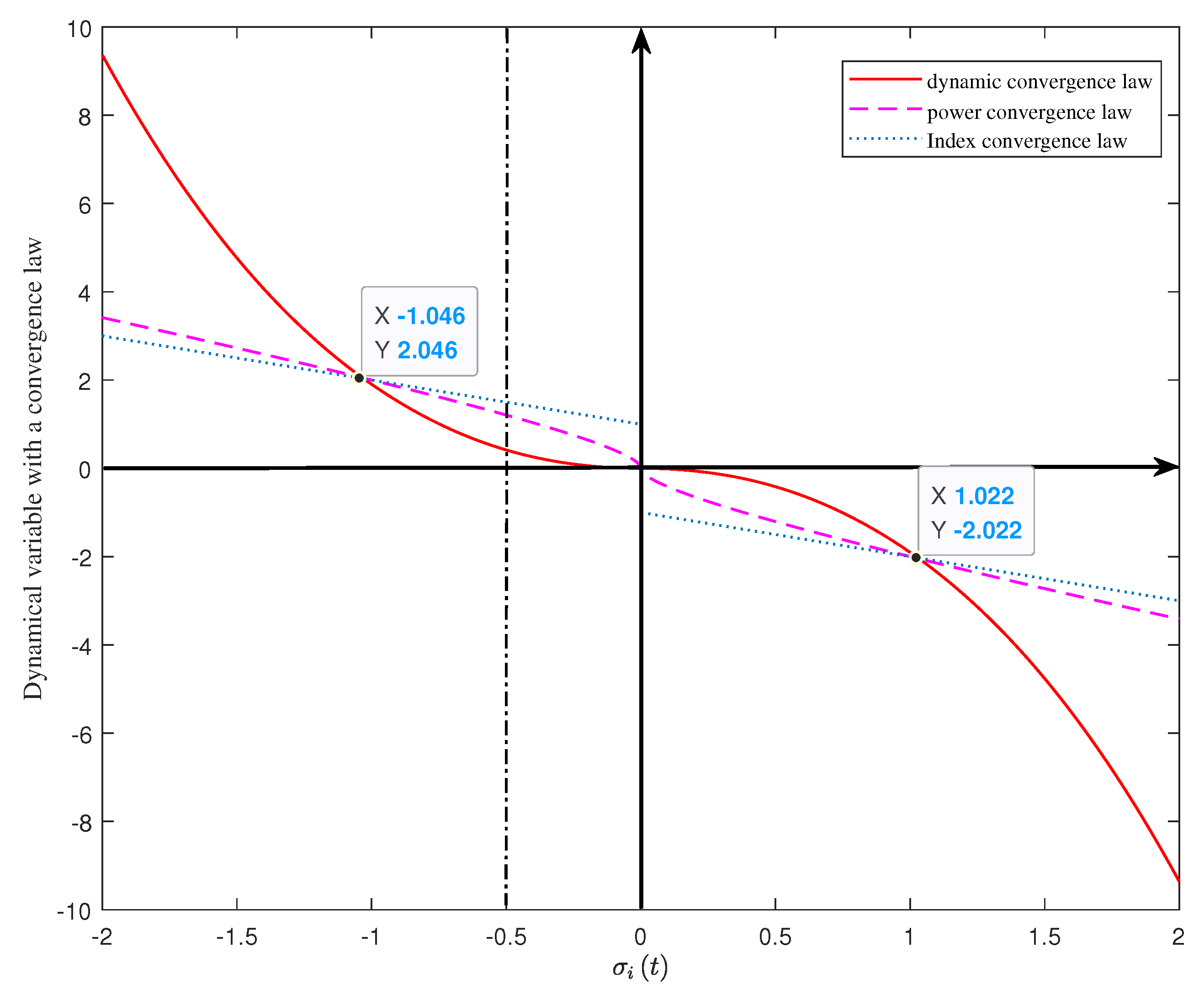
• Innovative Sliding Mode Control Design: Building on conventional sliding mode control, this paper develops a new sliding mode surface and convergence law. The refined convergence law decelerates the initiation of the arrival phase to reduce chattering, while simultaneously accelerating the system’s response as it moves away from the sliding mode surface. This dual effect enhances both the dynamic performance and responsiveness of the system.
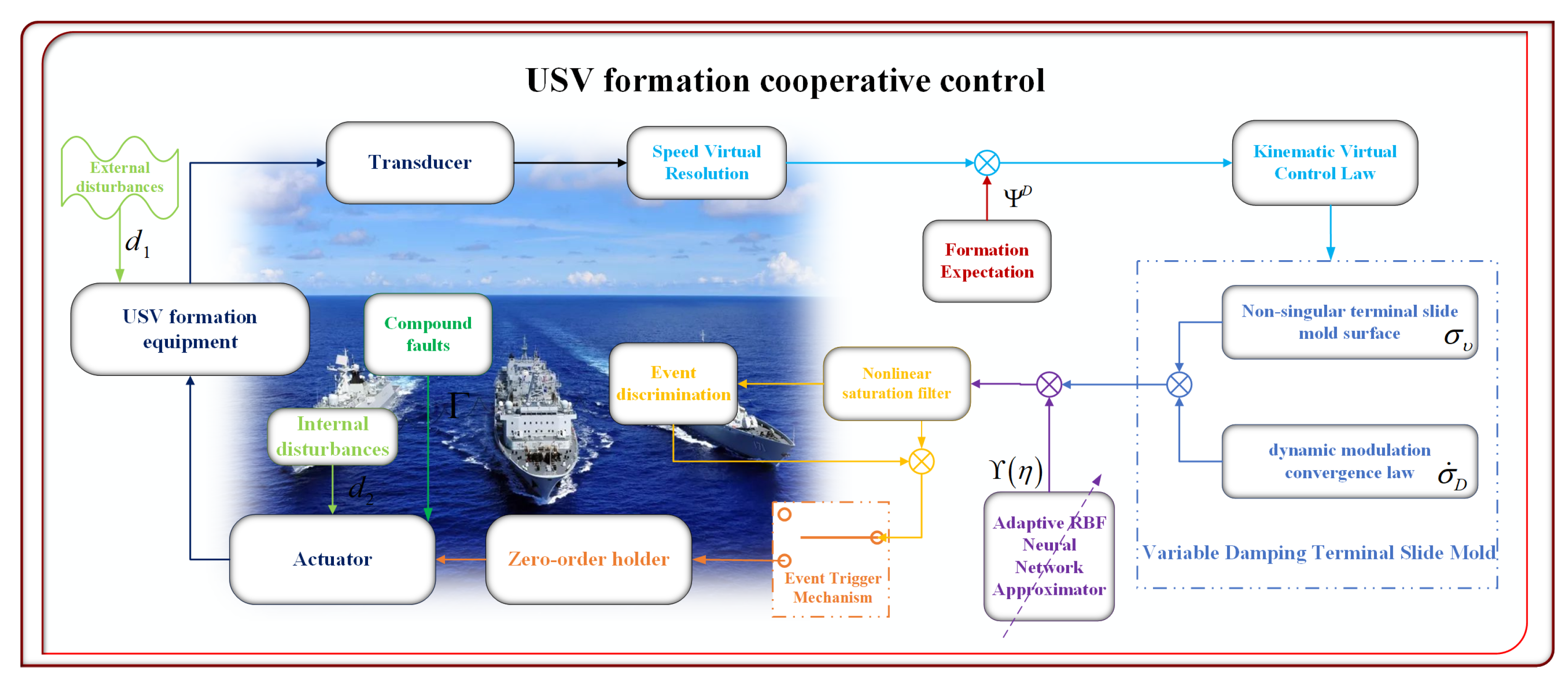
• Combination of Nonlinear Saturation Fitting and Event-Triggered Mechanism: To address issues related to saturation filtering and communication resource constraints, a nonlinear saturation fitting function is designed and integrated with an event-triggered mechanism. This combined solution effectively reduces the communication overhead, mitigates potential communication problems during fault events, and maintains system stability and precision under adverse fault conditions.

In conclusion, the control strategies and methods developed in this work effectively address the challenges associated with controlling systems under complex fault conditions and limited communication resources. These contributions significantly enhance the robustness, response speed, and resource efficiency of automatic control systems, offering both valuable theoretical insights and practical guidance for related research and applications.

2. Problem Formulation

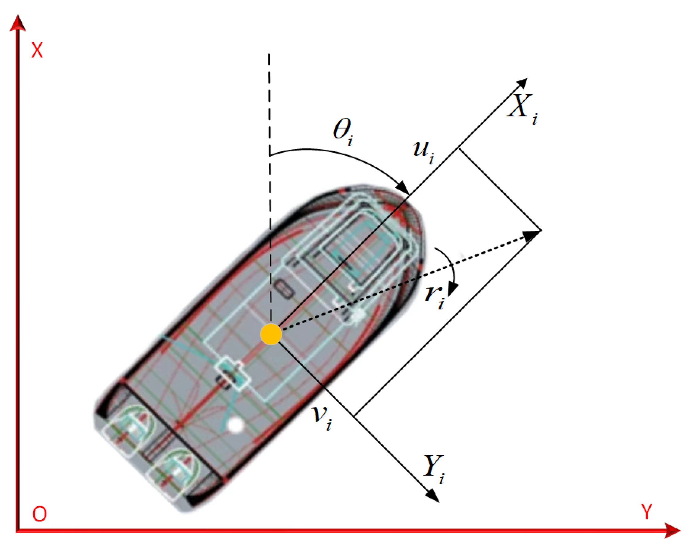
2.1. Mathematical Model

In this paper, we consider the law of motion of the USV in the horizontal plane, where the mass of the USV is uniformly distributed [33]. The kinematic characteristics of the USV [34] in the inertial coordinate system are shown in Figure 1.

The kinematics equation of the USV is described as

$${\dot{\eta }}_i=J_i\left({\theta }_i\right){\upsilon }_i$$

(1)

where $J_i\left({\theta }_i\right)=\left[cos\left({\theta }_i\right),-sin\left({\theta }_i\right),0;sin\left({\theta }_i\right),cos\left({\theta }_i\right),0;0,0,1\right]$. $\eta$ is the position coordinate vector, ${\dot{\eta }}_i={[{\dot{x}}_i,{\dot{y}}_i,{\dot{\theta }}_i]}^T$.

The dynamics equation of the USV is described as

$$M_i{\dot{\upsilon }}_i=-C_i\left({\upsilon }_i\right){\upsilon }_i-D_i{\upsilon }_i+{\tau }_i+d_i$$

(2)

where ${\upsilon }_i={[u_i,v_i,r_i]}^T$ is the velocity vector, ${\tau }_i$ is the control input, $d_i$ represents unknown external disturbances, $∥d∥\le d_{max}$. $M_i$ is the symmetric positive definite inertia matrix, $C_i\left({\upsilon }_i\right)$ denotes the centripetal and Coriolis torques, and $D_i$ is the damping matrix.

The motion model of the USV has systematic uptake, which can be expressed as

$${\dot{\upsilon }}_i=-M_i^{-1}{C}_i\left({\upsilon }_i\right){\upsilon }_i-M_i^{-1}{D}_i{\upsilon }_i+M_i^{-1}{\tau }_i+M_i^{-1}{d}_i$$

(3)

To facilitate the kinetic description, Equation (2) is transformed to

$${\dot{\upsilon }}_i=-{\Delta }_i+M_i^{-1}{\tau }_i+M_i^{-1}{d}_i$$

(4)

where ${\Delta }_i=M_i^{-1}\left(C_i\left({\upsilon }_i\right)+D_i\right){\upsilon }_i$ is the model parameter uncertainty term.

2.2. Fault Model

When a USV experiences an actuator failure, the actuator cannot execute the input command correctly; in other words, it cannot execute the control signal correctly. This issue will surely affect the control performance of the USV and thus impact the entire formation control. Actuator faults can be described as

$${\tau }_i^{*}={\Gamma }_i{\tau }_i\left(t\right)+f_i$$

(5)

where ${\Gamma }_i$ is the partial failure efficiency factor, $f={\left[f_1,f_2,f_3\right]}^{\mathrm{T}}$ is the deviation fault, ${\tau }_i$ is the actual control input to the system, ${\tau }_i^{*}$ is the input signal affected by the actuator fault, and ${\tau }_i^{*}\in {\mathrm{R}}^{3\times 1}$.

Assumption 1.

A partial failure fault satisfies condition $0<{\Gamma }_i\le 1$, $i=1,2,3$, ensuring that faults do not completely disable the system and allowing the control law to compensate for them.

Remark 1.

During actual formation sailing, devices are bound by physical constraints such as actuator power ratings and limited shipboard power sources. Consequently, the control inputs are subject to saturation constraints. Therefore, it is necessary to introduce a saturation function to model this physical characteristic. The control input can thus be redefined as

$${\tau }_{bi}=sat\left({\tau }_i^{*}\right)=\left\{\begin{array}{c}{\tau }_i^{*},\\ {\tau }_M,\end{array}\right.\begin{array}{c}∥{\tau }_i^{*}∥\le {\tau }_M\\ {\tau }_M\le {\tau }_i^{*}\end{array}$$

(6)

where ${\tau }_M>0$ is the maximum control force and moment provided by the USV propulsion system, and $sat\left(·\right)$ is the saturation function.

Lemma 1

([35]). Integral Valuation Theorem. $m_A\left(b-a\right)\le {\int }_a^{b}Adt\le M_A\left(b-a\right)$, $m_A$ and $M_A$ are the minimum and maximum values of A.

Lemma 2

([36]). $-ln\left(1+x\right)\le -{\displaystyle \frac{\left|x\right|}{1+\left|x\right|}}\le -{\displaystyle \frac{c_b{\left|x\right|}^{\frac{1}{2}}-\frac{1}{2}{c}_b^2}{1+\left|x\right|}}$, $c_b>0.25$.

Lemma 3

([37]). Select $N_{\kappa }\left(Q_{\kappa }\right)=exp({(Q_{\kappa }-\kappa )}^{\mathrm{T}}(Q_{\kappa }-\kappa )/-l^2)$ as the Gaussian function to improve nonlinear local approximation. $W_{\kappa }^{*}$ is the best-fitting $m_{\kappa }$-dimensional weighted row vector, shown as

$$W_{\kappa }^{*}=arg\left({min}_{{\stackrel{⌢}{W}}_{\kappa }^{*}}\left\{\underset{Q_{\kappa }\in {\Xi }^{m_{\kappa }}}{sup}\left|{\stackrel{⌢}{W}}_{\kappa }^{*T}{\zeta }_{\kappa }\left(Q_{\kappa }\right)-f_{\kappa }\left(Q_{\kappa }\right)\right|\right\}\right)$$

2.3. Cooperative Formation Model

Equations (1) and (4) are simplified using state-space equations in matrix form derived from kinematics and dynamics. Meanwhile, the global motion model of the USV cooperative formation (7), which takes into account perturbations and uncertainties in the model parameters, is established by integrating the saturation function (6)

$$\left\{\begin{array}{c}{\dot{\eta }}_i=J_i\left({\theta }_i\right){\upsilon }_i\\ {\dot{\upsilon }}_i=-{\Delta }_i+sat\left({\tau }_i^{*}\right)+M_i^{-1}{d}_i\end{array}\right.$$

(7)

where $i=L\in \left\{L_1,L_2,\cdots ,L_n\right\}$ is the leader device, and $i=f\in \left\{f_1,f_2,\cdots ,f_m\right\}$ is the follower device.

The real cooperative formation geometric feature matrix of the leader ship and the follower ship in the global coordinate system is ${\Psi }_{lf}=\left[L_{lf};{\Phi }_{lf};{\Phi }_{fl}\right]$, where $L_{lf}$ is the generalized distance between the leader and the follower, and ${\Phi }_{lf}$ is the angle between the leader and $L_{lf}$. $L_{lf}^D$ is the desired formation geometric distance between the leader and follower ships, $L_{lf}^D\ge ∥L_{lf}^D∥$, and $∥L_{lf}^D∥$ indicates the minimum safe distance. ${\Phi }_{fl}^D$ is the desired angle between the follower ship and $L_{lf}^D$. The geometric relationship between the leader ship and the follower ship in the generalized spatial coordinates is illustrated in Figure 2.

Cooperative formation control has two phases: recovery and keeping. This aims to change the shape of the group from ${\Psi }_{lf}$ to ${\Psi }_{lf}^D$ in space, while keeping it together. The dynamic feature represents the target motion synergy as $\underset{t\to \infty }{\lim }\left({\Psi }_{lf}^D-{\Psi }_{lf}\right)=0$, establishing the positional dynamics of each device and the dynamic transformation feature relationship as

$${\dot{\eta }}_l={\dot{\eta }}_f+G_{\dot{\eta }lf}=\left[\begin{array}{c}{\dot{x}}_l\\ {\dot{y}}_l\\ {\dot{\theta }}_l\end{array}\right]=\left[\begin{array}{c}{\dot{x}}_f\\ {\dot{y}}_f\\ {\dot{\theta }}_f\end{array}\right]+\left[\begin{array}{c}{G}_{\dot{x}lf}\\ G_{\dot{y}lf}\\ G_{\dot{\theta }lf}\end{array}\right]$$

(8)

where $G_{\dot{x}lf}={\dot{L}}_{lf}cos\left({\theta }_l+{\Phi }_{lf}\right)+L_{lf}\left({\dot{\theta }}_l+{\dot{\Phi }}_{lf}\right)sin\left({\theta }_l+{\Phi }_{lf}\right)$; $G_{\dot{y}lf}=-{\dot{L}}_{lf}sin\left({\theta }_l+{\Phi }_{lf}\right)-L_{lf}\left({\dot{\theta }}_l+{\dot{\Phi }}_{lf}\right)cos\left({\theta }_l+{\Phi }_{lf}\right)$ and $G_{\dot{\theta }lf}={\dot{\Phi }}_{lf}+{\dot{\Phi }}_{fl}$ are the motion transition terms.

After collation, the formation motion difference model (9) is used to control the formation. This matrix is used to design the control system to achieve objective $\underset{t\to \infty }{\lim }{\eta }_i^E=0$.

$${\eta }_i^E={\eta }_i^D-{\eta }_i=\left[\begin{array}{c}{\eta }_l^d\\ {\eta }_f^d\\ {\overline{\eta }}_l^d\\ {\overline{\eta }}_f^d\end{array}\right]-\left[\begin{array}{c}{\eta }_l\\ {\eta }_f\\ {\overline{\eta }}_l\\ {\overline{\eta }}_f\end{array}\right]$$

(9)

where ${\eta }_l^d$ is the geometric positional expectation of the lead ship, and ${\eta }_f^d$ is the expectation of the follower ship. ${\overline{\eta }}_l^d$ is the virtual expectation of ${\overline{\eta }}_l$, and ${\overline{\eta }}_f^d$ is the virtual expectation of ${\overline{\eta }}_f$.

Equation (9) and the cooperative formation model (7) are used to derive the dynamic model (10).

$${\dot{E}}_{\eta i}={\dot{\eta }}_i^d-{\dot{\eta }}_i$$

(10)

3. Basic Control Design

3.1. Non-Singular Terminal Sliding Mode Surface Design and Analysis

Based on the conventional TSMC strategy [38], a novel TSMS is designed based on the traditional terminal slide mold surface.

$${\sigma }_{\upsilon i}=c_1{E}_{\upsilon i}+c_2\int {∥E_{\upsilon i}∥}^{c_4}sign\left[E_{\upsilon i}\right]dt+c_3{∥E_{\upsilon i}∥}^{c_5}sign\left[E_{\upsilon i}\right]$$

(11)

where $c_1$, $c_2$, $c_3$, $c_4$, $c_5$ are normal number diagonal matrices and $sign\left[·\right]$ is the sign diagonal matrix. Integral term $\int {∥E_{\upsilon i}∥}^{c_4}sign\left[E_{\upsilon i}\right]dt$ introduces historical error information, which can smooth the control signal, and power exponent term ${∥E_{\upsilon i}∥}^{c_5}sign\left[E_{\upsilon i}\right]$ dynamically adjusts the control effort, so that, when the error is small, the sliding mode surface changes smoothly, thus reducing the risk of chattering. Deriving Equation (11) gives Equation (12).

$${\dot{\sigma }}_{\upsilon i}=\left(c_1+c_3{c}_5{∥E_{\upsilon i}∥}^{c_5-1}sign\left[E_{\upsilon i}\right]\right){\dot{E}}_{\upsilon i}+c_2{∥E_{\upsilon i}∥}^{c_4}sign\left[E_{\upsilon i}\right]$$

(12)

According to [39], it can be seen that there is no singularity in ${\dot{\sigma }}_{\upsilon i}$, and the SMS satisfies Equation (13). Therefore, the novel SMS is not affected by the singularity.

$$\left\{\begin{array}{c}{\sigma }_{\upsilon i}>0,E_{\upsilon i}>0\\ {\sigma }_{\upsilon i}=0,E_{\upsilon i}=0\\ {\sigma }_{\upsilon i}<0,E_{\upsilon i}<0\end{array}\right.$$

(13)

Proof. 

When ${\sigma }_{\upsilon i}=0$, ${\dot{\sigma }}_{\upsilon i}={\displaystyle \frac{d{\sigma }_{\upsilon i}}{dt}}=0$, Equation (12) can be deformed into

$${\dot{E}}_{\upsilon i}={\displaystyle \frac{d{E}_{\upsilon i}}{dt}}=-{\displaystyle \frac{c_2{∥E_{\upsilon i}∥}^{c_4}sign\left[E_{\upsilon i}\right]}{c_1+c_3{c}_5{∥E_{\upsilon i}∥}^{c_5-1}sign\left[E_{\upsilon i}\right]}}$$

(14)

Integrating Equation (14) in the convergence interval $\left(0,T_{\upsilon }\right)$ yields

$$-T_{\upsilon }={\int }_0^{E_{\upsilon i}\left(T_{\upsilon }\right)}{\displaystyle \frac{c_1+c_3{c}_5{∥E_{\upsilon i}∥}^{c_5-1}sign\left[E_{\upsilon i}\right]}{c_2{∥E∥}^{c_4}sign\left[E_{\upsilon i}\right]}}d{E}_{\upsilon i}=c_2^{-1}{\int }_0^{E_{\upsilon i}\left(T_{\upsilon }\right)}{\displaystyle \frac{c_{1}sign\left[E_{\upsilon i}\right]}{{∥E_{\upsilon i}∥}^{c_4}}}+c_3{c}_5∥E_{\upsilon i}∥d{E}_{\upsilon i}$$

(15)

According to Lemma 1, it is known that $m_{\upsilon e}(T_{\upsilon }-0)\le {\int }_0^{T_{\upsilon }}{c}_3{c}_5{∥E_{\upsilon i}∥}^{c_5-1}dt\le M_{\upsilon e}(T_{\upsilon }-0)$. When $E_{\upsilon i}\left(T_{\upsilon }\right)=0$, then ${\int }_0^{E_{\upsilon i}\left(T_{\upsilon }\right)}{c}_3{c}_5∥E_{\upsilon i}∥d{E}_{\upsilon i}=c_3{c}_5\left[E_{\upsilon i}{\left(T_{\upsilon }\right)}^{2}sign\left(E_{\upsilon i}\left(T_{\upsilon }\right)\right)-0\right]=0$, and Equation (15) is deformed into

$$-T_{\upsilon }=c_2^{-1}{\int }_0^{E_{\upsilon i}\left(T_{\upsilon }\right)}{c}_1{\displaystyle \frac{sign\left[E_{\upsilon i}\right]}{{∥E_{\upsilon i}∥}^{c_4}}}d{E}_{\upsilon i}\ge c_2^{-1}{\int }_0^{E_{\upsilon i}\left(T_{\upsilon }\right)}{c}_1{∥E_{\upsilon i}∥}^{c_4}d{E}_{\upsilon i}\ge -c_2^{-1}{c}_1{∥E_{\upsilon i}\left(0\right)∥}^{1-c_4}$$

(16)

Up to this point, it can be seen that the TSMS can complete convergence in a finite time $T_{\upsilon }\le c_1{c}_2^{-1}{∥E_{\upsilon i}\left(0\right)∥}^{1-c_4}$. □

3.2. Dynamically Regulated Convergence Law Design and Analysis

To optimize chattering and improve the robustness, a novel dynamically regulated convergence law (17) is designed based on the traditional power convergence law.

$${\dot{\sigma }}_{Di}=-\epsilon \left[\left(k+{\sigma }_{\upsilon i}^2\right)ln\left(k+{\sigma }_{\upsilon i}^2\right)-kln\left(k\right)\right]sign\left[{\sigma }_{\upsilon i}\right]-{\kappa }_{\upsilon i}{\sigma }_{\upsilon i}$$

(17)

where $\epsilon >0$, $k\ge 1$, ${\kappa }_{\upsilon i}>0$.

Proof. 

When $D=\left(k+{\sigma }_{\upsilon i}^2\right)ln\left(k+{\sigma }_{\upsilon i}^2\right)-kln\left(k\right)$, considering Lemma 2, then $-D\le -\left(k-1+{∥{\sigma }_{\upsilon i}∥}^2\right)+kln\left(k\right)\le -\left(k-1+c_b∥{\sigma }_{\upsilon i}∥-{\displaystyle \frac{1}{2}}{c}_b^2\right)+kln\left(k\right)$.

Obtain ${\dot{\sigma }}_D=-\epsilon \left[\left(k-1+c_b∥{\sigma }_{\upsilon i}∥-{\displaystyle \frac{1}{2}}{c}_b^2\right)-kln\left(k\right)\right]sign\left[{\sigma }_{\upsilon i}\right]$. Establishing the Lyapunov function $V_D={\displaystyle \frac{1}{2}}{\left({\sigma }_{\upsilon i}^{\mathrm{T}}{\sigma }_{\upsilon i}\right)}^2$ and bringing in Equation (17), ${\dot{V}}_D$ can be obtained:

$$\begin{array}{cc}\hfill & {\dot{V}}_D=-{\sigma }_{\upsilon i}^{\mathrm{T}}{\sigma }_{\upsilon i}{\sigma }_{\upsilon i}^{\mathrm{T}}(\epsilon \left[\left(k+{\sigma }_{\upsilon i}^2\right)ln\left(k+{\sigma }_{\upsilon i}^2\right)-kln\left(k\right)\right]sign\left[{\sigma }_{\upsilon i}\right]+\kappa {\sigma }_{\upsilon i})\hfill \\ \hfill & \le -{\sigma }_{\upsilon i}^{\mathrm{T}}{\sigma }_{\upsilon i}[\epsilon ∥{\sigma }_{\upsilon i}^{\mathrm{T}}∥(k-1+c_b∥{\sigma }_{\upsilon i}∥-{\displaystyle \frac{1}{2}}{c}_b^2)-kln\left(k\right)\epsilon {\sigma }_{\upsilon i}^{\mathrm{T}}]\hfill \\ \hfill & \le -{\epsilon }_D{V}_D-{\epsilon }^{*}{\dot{V}}_D^{{\displaystyle \frac{3}{4}}}\hfill \end{array}$$

(18)

where ${\epsilon }^{*}=min\left\{c_b-kln\left(k\right)\epsilon \right\}$, $c_b-kln\left(k\right)\epsilon >0$, ${\epsilon }_D=min\left\{\epsilon -{\displaystyle \frac{1}{2}}\epsilon c_b^2\right\}$, $\epsilon -{\displaystyle \frac{1}{2}}\epsilon c_b^2>0$.

Thus, it can be shown that the dynamically regulated convergence law can realize finite-time convergence. A comparison of the sliding mode convergence law is shown in Figure 3. □

3.3. Event-Triggering Mechanism Design and Stability Analysis

The wireless communication system is used to manage the polling waste issue in the server event access mechanism caused by actuator failures. To effectively reduce unnecessary control updates, the event trigger mechanism of the upper computer is designed as follows:

$$\left\{\begin{array}{c}{\tau }_i={\tau }_{i,c},\forall t\in \left[t_c,t_{c+1}\right)\\ {\tau }_{i,c}=inf\left\{{\tau }_i,∥{\zeta }_{i\tau }∥\ge {\chi }_{i,c}∥{\tau }_i∥+{\xi }_{i,c}\mathrm{or}t-t_c\ge T_{max}\right\}\end{array}\right.$$

(19)

where ${\zeta }_{i,c}={\tau }_i-{\tau }_{i,c}$; conditional weight $0<{\chi }_{i,c}<1$, $∥{\xi }_{i,c}∥\ge 0$, is the control value updated by the controller. $t_c,c\in R^{+}$ is the trigger time; it can send the updated control command if the trigger mechanism is satisfied. $T_{max}$ is the upper limit of the sampling period. When the trigger is not satisfied, the device executes the control command of the zero-order keeper in $\left[t_c,t_{c+1}\right)$ time.

To achieve dynamic fault-tolerant control within the performance limits, a hyperbolic tangent smooth function $sat\left(·\right)$ is introduced based on Equation (10). The saturation filtering mechanism is designed as follows:

$${\tau }_{i,c}=L_{id}tanh\left({\tau }_i\right)+E_{ic}$$

(20)

where $E_{ic}$ is the filtering error.

Proof. 

If the designed mechanism threshold is less than a neighborhood, the Zeno problem occurs and the controller will output frequently, affecting the control stability. Therefore, the trigger interval is made to be $∥t_{c+1}-t_c∥>t_u,t_u\in {\mathrm{N}}^{+}$ to avoid the Zeno phenomenon.

According to Equation (20), the input signal is characterized by the presence of $∥{\tau }_i∥\le {\tau }_M$ through the saturation filtering mechanism, which leads to $∥{\zeta }_{i\tau }∥=∥{\tau }_i-{\tau }_{i,c}∥\le \tau ,\tau >0$. This shows that the output of the twice-triggered controller is a bounded variable.

Deriving the trigger error ${\zeta }_{i\tau }$ with respect to time yields

$${\displaystyle \frac{d∥{\zeta }_{i\tau }∥}{dt}}=\mathrm{sign}\left[{\dot{\zeta }}_{i\tau }\right]{\dot{\zeta }}_{i\tau }\le {\displaystyle \frac{d∥L_{id}tanh\left({\tau }_i\right)+E_{ic}∥}{dt}}$$

(21)

The input is constrained to saturation ${\tau }_M$, which, according to Equation (21), yields

$$\begin{array}{cc}\hfill \left({\chi }_{i,c}∥{\tau }_i∥+{\xi }_{i,c}\right){\left({\tau }_M{t}_u\right)}^{-1}& \le \left(\underset{t\to t_{c+1}}{lim}{\zeta }_{i\tau }\left(t\right)-{\zeta }_{i\tau }\left(t_c\right)\right){\left({\tau }_M{t}_u\right)}^{-1}\hfill \\ \hfill & \le {\left({\tau }_M{t}_u\right)}^{-1}d{\zeta }_{i\tau }\le \left(t_{c+1}-t_c\right)t_u^{-1}.\hfill \end{array}$$

Thus, $inf\left\{t_u\right\}=\left({\chi }_{i,c}∥{\tau }_i∥+{\xi }_{i,c}\right)/\left({\tau }_M{t}_u\right)$ is obtained, proving that the event-triggered mechanism is able to avoid Zeno’s phenomenon. □

3.4. Controller Design

The position error is defined as

$$E_{qi}=\left[\begin{array}{c}{E}_{qxi}\\ E_{qyi}\\ E_{q\theta i}\end{array}\right]=G_a{E}_{\eta i}-G_{\eta i}$$

(22)

where $G_a=\left[1,0,0;0,1,0;0,0,0\right]$, $G_{\eta i}={\left[-cos\left({\theta }_e\right),-{\theta }_e,{\left(1-cos\left({\theta }_e\right)\right)}^{{\displaystyle \frac{1}{2}}}\right]}^{\mathrm{T}}$.

The virtual control laws can be designed as follows:

$${\upsilon }_i=W_{qi}{E}_{qi}+W_{Ei}$$

(23)

where $W_{Ei}={\left[-1-u{E}_{qx}-r{\theta }_e+u,\beta usin\left({\theta }_e\right)+r,D_i\left({\sigma }_{\upsilon i}\right)sign\left[{\sigma }_{\upsilon i}\right]+{\eta }_f^d\right]}^{\mathrm{T}}$, $W_{qi}=\left[k_{l2}{\alpha }_{fx},0,0;0,{\rho }_l{k}_{l1}{\alpha }_{fy},0;0,0,{\alpha }_{f\theta }\right]$, $D_i\left({\sigma }_{\upsilon i}\right)=\left(k+{\sigma }_{\upsilon i}^2\right)ln\left(k+{\sigma }_{\upsilon i}^2\right)-kln\left(k\right)$, ${\rho }_l$, $\beta$, ${\alpha }_{fx}$, ${\alpha }_{fy}$ and ${\alpha }_{f\theta }$ are positive constants.

Lemma 3 is used to construct the RBF neural network approximator as ${\Delta }_i=W_i^{*\mathrm{T}}{Z}_{Wi}\left({\upsilon }_i\right)+e_i\left({\upsilon }_i\right)$. Substituting Equation (10) leads to

$${\dot{E}}_{\upsilon i}={\dot{\overline{\upsilon }}}_i^d-\left(M_i^{-1}{\tau }_i-W_i^{*\mathrm{T}}{Z}_{Wi}\left({\upsilon }_i\right)-e_i\left({\upsilon }_i\right)-M_i^{-1}{d}_i\right)$$

(24)

Substituting Equation (24) into Equation (12) yields

$$\begin{array}{cc}\hfill {\dot{\sigma }}_{\upsilon i}& =A_1{\dot{E}}_{\upsilon i}+c_2{∥E_{\upsilon i}∥}^{{\displaystyle \frac{1}{4}}}sign\left[E_{\upsilon i}\right]\hfill \\ \hfill & =A_1\left({\dot{\overline{\upsilon }}}_i^d-\left(M_i^{-1}{\tau }_i-W_i^{*\mathrm{T}}{Z}_{Wi}\left({\upsilon }_i\right)-e_i\left({\upsilon }_i\right)-M_i^{-1}{d}_i\right)\right)+A_3\hfill \end{array}$$

(25)

where $A_1=c_1+c_3{c}_5{∥E_{\upsilon i}∥}^{{\displaystyle \frac{5}{4}}}sign\left[E_{\upsilon i}\right]$, $A_2=k+ln{\left(k+{∥{\sigma }_{\upsilon i}∥}^2\right)}^{{∥{\sigma }_{\upsilon i}∥}^2-1}$, $A_3=c_2{∥E_{\upsilon i}∥}^{c_4}sign\left[E_{\upsilon i}\right]$.

To make the sliding model more robust and converge faster, we substitute the novel TSMS and the dynamically regulated convergence law into the global motion model. The adaptive law and dynamic controller are obtained.

$${\dot{\widehat{\vartheta }}}_{\tau i}=C_1{\sigma }_{\upsilon i}tanh\left(C_2{\sigma }_{\upsilon i}\right)-C_4{\widehat{\vartheta }}_{\tau i}+C_3{∥{\sigma }_{\upsilon i}∥}^{2}tanh\left({\sigma }_{\upsilon }^2\right)P_d^4$$

(26)

$$\begin{array}{cc}\hfill {\tau }_i=& M_i{A}_1^{-1}\epsilon sign\left[{\sigma }_{\upsilon i}\right]A_{2}ln\left(k+{∥{\sigma }_i∥}^{-1}\right)+M_i{A}_1^{-1}{C}_1{\widehat{\vartheta }}_{\tau i}tanh\left(C_2{\sigma }_{\upsilon i}\right)\hfill \\ \hfill & +M_i{A}_1^{-1}{C}_3{\widehat{\vartheta }}_{\tau i}{\sigma }_{\upsilon i}{P}_d^4+M_i{\dot{\overline{\upsilon }}}_i^d\hfill \end{array}$$

(27)

where $C_1,C_2,C_3,C_4\in {\mathrm{R}}^{+}$. $∥{\vartheta }_{\tau i}∥\le {\overline{\vartheta }}_{\tau i}$. $P_d=∥M^{-1}{\tau }_{max}∥+∥Z\left({\upsilon }_i\right)∥+∥{\upsilon }_e∥+5$ is the continuous excitation. The design flowchart is shown in Figure 4.

3.5. Stability Analysis

Consider the system (7); $V_q={\displaystyle \frac{1}{2}}{E}_{qi}^{\mathrm{T}}{E}_{qi}$ is designed and the first-order derivation is obtained:

$$\begin{array}{cc}\hfill {\dot{V}}_q& =E_{qx}\left(-sin{\theta }_e+{\dot{x}}_e\right)+E_{qy}\left({\dot{y}}_e+{\dot{\theta }}_e\right)+E_{q\theta }\left({\displaystyle \frac{1}{2}}{\left(1-cos\left({\theta }_e\right)\right)}^{-{\displaystyle \frac{1}{2}}}\right)\left({\dot{\theta }}_{e}sin\left({\theta }_e\right)\right)\hfill \\ \hfill & =E_{qx}\left(ucos\left({\theta }_e\right)-u+E_{qy}r-{\theta }_{e}r\right)+E_{qy}\left(usin\left({\theta }_e\right)+{\dot{\theta }}_e-r{E}_{qx}\right)+{\dot{\theta }}_{e}sin\left({\theta }_e\right)\hfill \end{array}$$

(28)

Substituting the kinematic control law and transforming it using Young’s inequality yields

$$\begin{array}{cc}\hfill {\dot{V}}_q& \le -k_1^{{\displaystyle \frac{1}{2}}}∥E_{qx}∥-k_1{E}_{qx}^{\mathrm{T}}{E}_{qx}-\sqrt{\partial k_1}∥E_{qy}∥-\partial k_1{E}_{qy}^{\mathrm{T}}{E}_{qy}-k_2{E}_{q\theta }^{\mathrm{T}}{E}_{q\theta }-k_2{E}_{q\theta }+6\hfill \\ \hfill & \le -K_1{V}_q-K_2{V}_q^{{\displaystyle \frac{1}{2}}}+6\hfill \end{array}$$

(29)

where $k_1$ and $k_2$ are positive constants, $K_1=min\left\{k_1\right\}$, $K_2=min\left\{k_2\right\}$.

The kinematic controller follows Lyapunov’s theory, which makes the cooperative formation system stable in finite time.

According to the new sliding mode surface and the adaptive law, the design of the Lyapunov function $V_{\upsilon }={\displaystyle \frac{1}{2}}{\sigma }_{\upsilon i}^{\mathrm{T}}{\sigma }_{\upsilon i}+{\displaystyle \frac{1}{2}}{\tilde{\vartheta }}_{\tau i}^{\mathrm{T}}{\tilde{\vartheta }}_{\tau i}$, where $\tilde{\vartheta }={\vartheta }_{\tau i}-{\widehat{\vartheta }}_{\tau i}$, and the first-order derivation of it leads to

$$\begin{array}{cc}\hfill {\dot{V}}_{\upsilon }& ={\sigma }_{\upsilon i}^{\mathrm{T}}\left[A_3\right.+A_1\left.\left({\dot{\overline{\upsilon }}}_i^d-M_i^{-1}tanh\left({\tau }_i+{\iota }_i\right)+W_i^{*\mathrm{T}}{Z}_{Wi}\left({\upsilon }_i\right)+e_i\left({\upsilon }_i\right)+M_i^{-1}{d}_i\right)\right]+{\tilde{\vartheta }}_{\tau i}^{\mathrm{T}}{\dot{\tilde{\vartheta }}}_{\tau i}\hfill \\ \hfill & \le {\sigma }_{\upsilon i}^{\mathrm{T}}\left[A_3+A_1\right.\left.\left({\dot{\overline{\upsilon }}}_i^d-{\tau }_i-M_i^{-1}{\iota }_i+W_i^{*\mathrm{T}}{Z}_{Wi}\left({\upsilon }_i\right)+e_i\left({\upsilon }_i\right)+M_i^{-1}{d}_i\right)\right]+{\tilde{\vartheta }}_{\tau i}^{\mathrm{T}}{\dot{\tilde{\vartheta }}}_{\tau i}\hfill \end{array}$$

(30)

Combining the minimum learning parameter and the paradigm inequality approach, Equation (31) can be simplified as

$$\begin{array}{cc}\hfill {\dot{V}}_{\upsilon }\le & {\sigma }_{\upsilon i}^{\mathrm{T}}\left[A_1\left({\dot{\overline{\upsilon }}}_i^d-{\tau }_i+∥M_i^{-1}{\iota }_i∥+∥M_i^{-1}{E}_{id}∥+∥W_i^{*\mathrm{T}}∥∥Z_{Wi}\left({\upsilon }_i\right)∥+∥e_i\left({\upsilon }_i\right)∥+∥M_i^{-1}{d}_i∥\right)\right.\left.+A_3\right]\hfill \\ \hfill & +{\tilde{\vartheta }}_{\tau i}^{\mathrm{T}}{\dot{\tilde{\vartheta }}}_{\tau i}\hfill \end{array}$$

(31)

Substituting Equations (26) and (27) and combining Young’s inequality, we obtain

$$\begin{array}{cc}\hfill {\dot{V}}_{\upsilon }\le & -{\displaystyle \frac{1}{2}}\epsilon {∥{\sigma }_{\upsilon i}∥}^2-\epsilon \left(s_1-s_2\right)∥{\sigma }_{\upsilon i}∥+\epsilon s_2^2-{\sigma }_{\upsilon i}^{\mathrm{T}}{\vartheta }_{\tau i}{C}_{1}tanh\left(C_2{\sigma }_{\upsilon i}\right)+C_1∥{\sigma }_{\upsilon i}^{\mathrm{T}}∥{\vartheta }_{\tau i}\hfill \\ \hfill & -C_3{∥{\sigma }_{\upsilon i}∥}^2{\widehat{\vartheta }}_{\tau i}{P}_d^4+\left(4C_1^{-1}\right)∥{\sigma }_{\upsilon i}^{\mathrm{T}}∥{\vartheta }_{\tau i}{P}_d^2+C_4{\tilde{\vartheta }}_{\tau i}^{\mathrm{T}}{\widehat{\vartheta }}_{\tau i}-C_3{\tilde{\vartheta }}_{\tau i}^{\mathrm{T}}{∥{\sigma }_{\upsilon i}∥}^2{P}_d^4+{\tilde{\vartheta }}_{\tau i}^{\mathrm{T}}{\vartheta }_{\tau i}\hfill \end{array}$$

(32)

where $s_2>s_1$, $C_4>2$.

According to inequality ${\tilde{\vartheta }}_{\tau i}^{\mathrm{T}}{\widehat{\vartheta }}_{\tau i}\le {\tilde{\vartheta }}_{\tau i}^{\mathrm{T}}\left({\vartheta }_{\tau i}-{\tilde{\vartheta }}_{\tau i}^{\mathrm{T}}\right)\le {\displaystyle \frac{1}{2}}{\vartheta }_{\tau i}^2-{\displaystyle \frac{1}{2}}{\tilde{\vartheta }}_{\tau i}^{\mathrm{T}}{\tilde{\vartheta }}_{\tau i}$ and Lemma 2, Equation (33) can be simplified as

$$\begin{array}{cc}\hfill {\dot{V}}_{\upsilon }\le & {\displaystyle \frac{1}{2}}\epsilon {∥{\sigma }_{\upsilon i}∥}^2-\epsilon \left(s_1-s_2\right)∥{\sigma }_{\upsilon i}∥-\left({\displaystyle \frac{1}{4}}{C}_4-{\displaystyle \frac{1}{2}}\right){\tilde{\vartheta }}_{\tau i}^{\mathrm{T}}{\tilde{\vartheta }}_{\tau i}-{\displaystyle \frac{1}{4}}∥{\tilde{\vartheta }}_{\tau i}∥\hfill \\ \hfill & +\epsilon s_2^2+C_1{C}_2^{-1}{\vartheta }_{\tau i}+{\displaystyle \frac{1}{2}}{\tilde{\vartheta }}_{\tau i}^{\mathrm{T}}{\vartheta }_{\tau i}+{\displaystyle \frac{1}{2}}{C}_4{\vartheta }_{\tau i}^{\mathrm{T}}{\vartheta }_{\tau i}+{\displaystyle \frac{1}{16}}{C}_4\hfill \end{array}$$

(33)

Based on Equations (30) and (33), the Lyapunov function $V_D=V_q+V_{\upsilon }$ is established and its derivation leads to

$$\begin{array}{cc}\hfill {\dot{V}}_D\le & -K_1{V}_q-K_2{V}_q^{{\displaystyle \frac{1}{2}}}+6+{\displaystyle \frac{1}{2}}\epsilon {∥{\sigma }_{\upsilon i}∥}^2-\epsilon \left(s_1-s_2\right)∥{\sigma }_{\upsilon i}∥-\left({\displaystyle \frac{1}{4}}{C}_4-{\displaystyle \frac{1}{2}}\right){\tilde{\vartheta }}_{\tau i}^{\mathrm{T}}{\tilde{\vartheta }}_{\tau i}\hfill \\ \hfill & -{\displaystyle \frac{1}{4}}∥{\tilde{\vartheta }}_{\tau i}∥+\epsilon s_2^2+C_1{C}_2^{-1}{\vartheta }_{\tau i}+{\displaystyle \frac{1}{2}}{\tilde{\vartheta }}_{\tau i}^{\mathrm{T}}{\vartheta }_{\tau i}+{\displaystyle \frac{1}{2}}{C}_4{\vartheta }_{\tau i}^{\mathrm{T}}{\vartheta }_{\tau i}+{\displaystyle \frac{1}{16}}{C}_4\hfill \end{array}$$

(34)

This is simplified using the minimum learning parameter method [40] to obtain

$$\begin{array}{cc}\hfill {\dot{V}}_D& \le -{\chi }_1\left(∥{\sigma }_{\upsilon i}∥+∥{\tilde{\vartheta }}_{\upsilon i}∥+∥E_{qi}∥\right)-{\chi }_2\left({∥{\sigma }_{\upsilon i}∥}^2+{∥{\tilde{\vartheta }}_{\upsilon i}∥}^2+E_{qi}^{\mathrm{T}}{E}_{qi}\right)+\lambda \hfill \\ \hfill & \le -{\chi }_1{V}_D^{{\displaystyle \frac{1}{2}}}-{\chi }_2{V}_D+\lambda \hfill \end{array}$$

(35)

where ${\chi }_1=min\left\{\epsilon \left(s_1-s_2\right),0.25,K_2\right\}$, ${\chi }_2=min\left\{{\displaystyle \frac{\epsilon C_3}{2}},{\displaystyle \frac{C_4-2}{4}},K_1\right\}$, boundary term $\lambda =max\left\{C_3\epsilon s_2^2+C_1{C}_2^{-1}{\vartheta }_{\tau i}+{\displaystyle \frac{1}{2}}{\vartheta }_{\tau }^{\mathrm{T}}{\vartheta }_{\tau }+{\lambda }_1+2\right\}$, ${\lambda }_1={\displaystyle \frac{1}{16}}{C}_4+{\displaystyle \frac{1}{2}}\epsilon s_2^2+{\displaystyle \frac{1}{2}}{C}_4{\vartheta }_{\tau }^{\mathrm{T}}{\vartheta }_{\tau }$. The proof shows that Equation (35) satisfies Lemmas 1–2 and can converge in finite time.

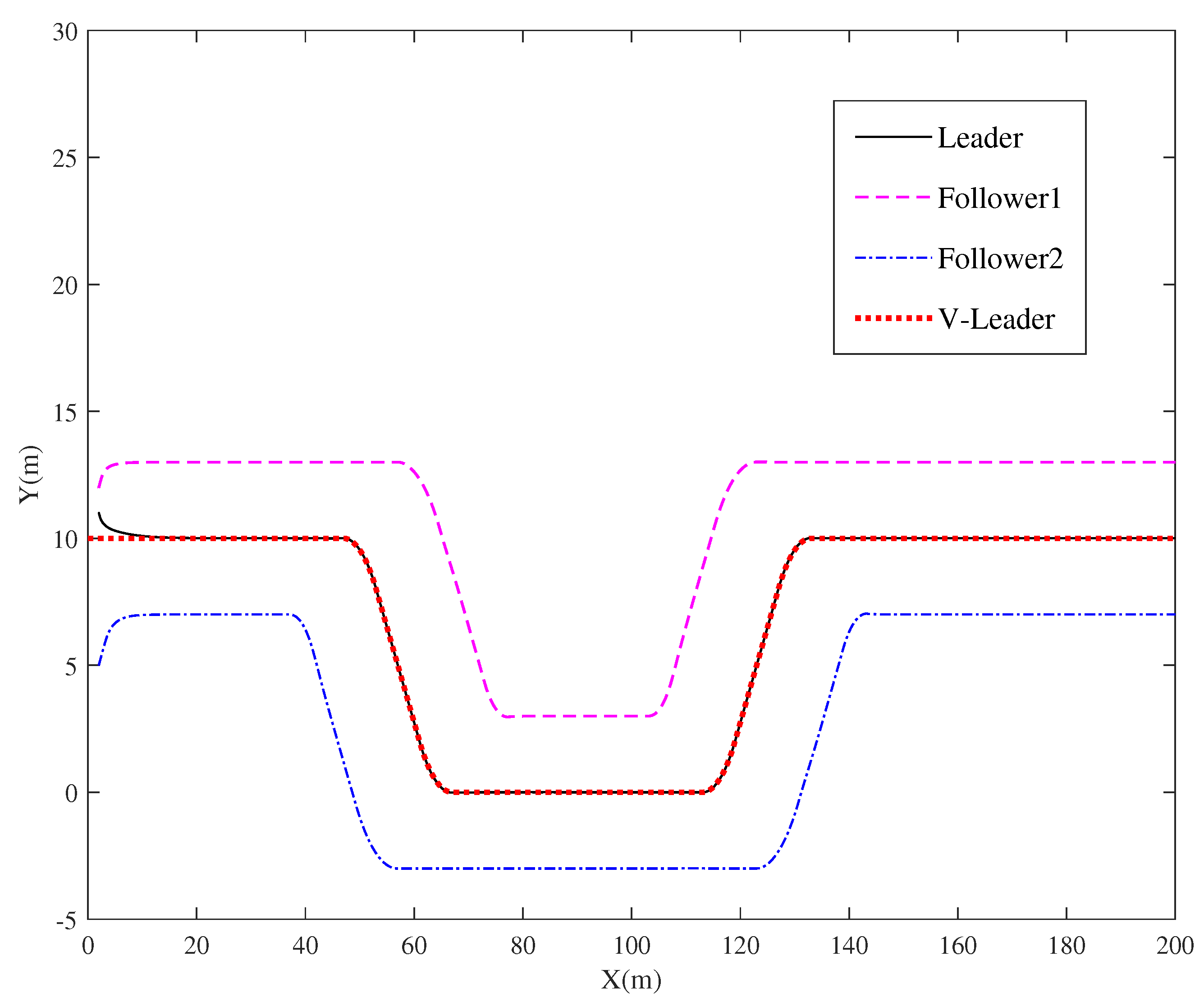
4. Simulation Analysis

For scientific simulation, all three USVs use CyberShip II [40], the 1:70 ship from the Norwegian University of Science and Technology with dual symmetrical propellers, dual rudders, and a single side thruster, with a mass of 23.8 kg, a length of 1.255 m, a breadth of 0.29 m, and the input limit value of ${\tau }_M={\left[5\mathrm{N},5\mathrm{N},2.5\mathrm{N}·\mathrm{m}\right]}^{\mathrm{T}}$. $d_{11}=12\mathrm{kg}/\mathrm{s}$, $d_{22}=17\mathrm{kg}/\mathrm{s}$, $d_{33}=0.5\mathrm{kg}/\mathrm{s}$, $d_{23}=d_{32}=0.2\mathrm{kg}/\mathrm{s}$, $m_{11}=25.8\mathrm{kg}$, $m_{22}=33.8\mathrm{kg}$, $m_{33}=2.76\mathrm{kg}$. The geometric features of the formation for the lead ship and two following ships are set to ${\Psi }_{lf1}=\left[3;90;90\right]$, ${\Psi }_{lf2}=\left[3.5;90;90\right]$. The virtual leader’s reference trajectory is ${\eta }_{l_0}={\left[x_l,y_l,{\theta }_l\right]}^{\mathrm{T}}$, where $x_l=t$, ${\theta }_l=arctan\left({\dot{x}}_l^{-1}{\dot{y}}_l\right)$, $y_l$ as follows [36].

The total simulation time is 200 s, and the step size is 0.01 s. In reality, actuators can exhibit intermittent failures; therefore, a random fault model is introduced: ${\Gamma }_i=\left\{\begin{array}{c}1\\ 0.6+G_{\omega }\end{array}\begin{array}{c},t\le 50\\ ,t>50\end{array}\right.$, $f_i=2$. Disturbances [40] to USVs caused by wind, waves, and currents are $d_i=\left[d_{iu},d_{iv},d_{ir}\right]$, where $d_{iu}=0.2sin\left(0.5t+{\displaystyle \frac{\pi }{4}}\right)+G_{\omega }$, $d_{iv}=0.18sin\left(0.5t\right)+0.1cos\left(t\right)+G_{\omega }$, $d_{ir}=0.25cos\left(t\right)+0.25G_{\omega }$, and $G_{\omega }$ denotes zero-mean Gaussian white noise, $d_{max}=2.5$.

To facilitate the verification of the control effect of USV cooperative formation, three USVs are selected to form a formation, with one of them as the leader and the other two as the followers. We set the initial offset to simulate the USV’s initial error; the initial position of the leader is ${\eta }_l\left(0\right)={\left[4,8,{1.8}^{-1}\pi \right]}^{\mathrm{T}}$, the initial position of the followers ${\eta }_{f_1}\left(0\right)={\left[3,7,{1.8}^{-1}\pi \right]}^{\mathrm{T}}$, ${\eta }_{f_2}\left(0\right)={\left[6,5,{1.8}^{-1}\pi \right]}^{\mathrm{T}}$, and the initial speed is set to 0 for all three USVs. Comparing the method of this paper with the traditional adaptive formation control method ${\tau }_{i1}$, an integral SMS ${\sigma }_{\upsilon i0}=c_1{E}_{\upsilon i}+c_2\int E_{\upsilon i}dt+c_3{\dot{E}}_{\upsilon i}$ [41] is introduced to verify the superiority of the algorithm. Then, combined with the exponential convergence law and without considering event-triggered control, the comparison controller is designed as

$${\tau }_{i0}=M_i{\delta }_i^{-1}\epsilon sign\left[{\sigma }_{\upsilon i0}\right]+M_i{\delta }_i^{-1}{C}_1{\widehat{\vartheta }}_{{\tau }_i}tanh\left(C_2{\sigma }_{\upsilon i0}\right)+M_i{\delta }_i^{-1}{C}_3{\widehat{\vartheta }}_{{\tau }_i}{\sigma }_{\upsilon i0}{P}_d^4+M_i{\dot{\overline{\eta }}}_i^d$$

(36)

The nodes of the RBF neural network function are uniformly set to 2, and the center is distributed in the interval $\left[-2,2\right]$. $T_{max}=2.5\mathrm{s}$. To verify the robustness of the control algorithm, the same control parameters are used for both controllers.

Table 1. Formation controller parameters.

Parameter	Value	Parameter	Value
${\epsilon }_u$	$0.5$	$C_{1u}$	10
${\epsilon }_v$	1	$C_{1v}$	25
${\epsilon }_r$	$0.05$	$C_{1r}$	17
$k_{l1}$	$0.2$	$C_{2u}$	$0.1$
$k_{l2}$	$2.5$	$C_{2v}$	15
${\rho }_l$	$0.4$	$C_{2r}$	$0.4$
${\alpha }_{fx}$	$0.15$	$C_{3u}$	180
${\alpha }_{fy}$	$0.1$	$C_{3v}$	130
${\alpha }_{f\theta }$	2	$C_{3r}$	40
$c_{i1}$	$diag\left(2,2.5,1.5\right)$	$C_{4u}$	1
$c_{i2}$	$diag\left(0.5,1,0.5\right)$	$C_{4v}$	1
$c_{i3}$	$diag\left(0.5,0.5,0.2\right)$	$C_{4r}$	$1.5$
${\chi }_{i,c}$	$0.1$	${\xi }_{i,c}$	$0.5$

represents the parameters of the formation controller.

To quantitatively assess the effectiveness of the algorithms in this paper, the following metrics are used: mean integral absolute control (MIAC) is used to calculate the input energy, and the mean integral squared error (MISE) is used to measure the error control accuracy, where $\mathrm{MIAC}={\left(t_l-t_0\right)}^{-1}{\int }_{t_0}^{t_l}∥{\tau }_i∥d\mu$, $\mathrm{MISE}={\left(t_l-t_0\right)}^{-1}{\int }_{t_0}^{t_l}{∥E_D∥}^{2}d\mu$.

Figure 5 demonstrates that the proposed control method effectively operates during both the formation recovery and holding phases, successfully navigating through width-varying narrows even in the presence of a partial actuator failure, multi-source interference, and input saturation. A quantitative comparison of the MISE is presented in Figure 6, Figure 7 and Figure 8 and

Table 2. ${\tau }_i$ quantitative analysis of control effect.

Evaluation Criterion	MIAC	MISE	Number of Transmissions
Leader	$\left[0.8,1.19,2.66\right]$	$\left[3.62,3.32,4.60\right]$	$\left[7980,8610,9280\right]$
Follower 1	$\left[0.9,1.69,2.21\right]$	$\left[3.35,2.82,2.02\right]$	$\left[8433,9106,9686\right]$
Follower 2	$\left[1.1,1.09,2.16\right]$	$\left[3.10,2.93,2.66\right]$	$\left[6621,7638,8370\right]$

and

Table 3. ${\tau }_{i0}$ quantitative analysis of control effect.

Evaluation Criterion	MIAC	MISE	Number of Transmissions
Leader	$\left[1.8,2.37,4.06\right]$	$\left[4.12,4.01,4.71\right]$	20,000
Follower 1	$\left[1.2,3.71,4.22\right]$	$\left[4.27,3.46,2.52\right]$	20,000
Follower 2	$\left[1.91,2.52,3.14\right]$	$\left[3.87,3.73,2.81\right]$	20,000

. It indicates that the proposed control law ${\tau }_i$ delivers superior control accuracy compared to ${\tau }_{i0}$. Notably, all control objects achieve the desired positions within 20 s, which is a significant improvement over ${\tau }_{i0}$ and ${\tau }_{i1}$, which require longer convergence times. The proposed method converges the position error to zero more rapidly and ensures smoother sailing at trajectory inflection points. Even under actuator failure, the jitter amplitude remains small, yielding higher overall control accuracy. An analysis of the leader’s position error further reveals that, in comparison to ${\tau }_{i0}$, the proposed method achieves better control at the inflection points between 45–65 s and 110–125 s by effectively suppressing error fluctuations, with no pronounced sharp deviations observed between 126 and 134 s. Moreover, relative to ${\tau }_{i1}$, the proposed approach exhibits faster initial error convergence and, during the intervals of 54–64 s and 125–140 s, demonstrates superior control accuracy and reduced error fluctuations in the presence of environmental disturbances and actuator faults. Similar improvements are observed for the follower vessels, where the proposed method enables faster formation adjustments in the early stages of navigation, avoids the typical buffeting observed with traditional sliding mode control, and yields enhanced error convergence at trajectory inflection points. In contrast, ${\tau }_{i1}$ is susceptible to abrupt positional and angular deviations due to actuator failure, a drawback not exhibited by ${\tau }_i$ throughout the entire voyage. Overall, the USVs, starting from different initial conditions, can all reach their desired states in finite time. This insensitivity to the initial conditions, combined with a moderate convergence rate, ensures accurate formation control while simultaneously mitigating chattering and excessive computational burdens, thereby underscoring the robustness and reliability of the proposed method.

Figure 9, Figure 10 and Figure 11 depict the dynamic curvature changes associated with speed errors across three degrees of freedom during cooperative formation operations. Analyzing the error convergence speed, stability, disturbance rejection, and stationarity reveals that ${\tau }_i$ exhibits clear advantages. First, regarding the convergence speed, ${\tau }_i$ reduces the error to near zero more rapidly than ${\tau }_{i0}$ and ${\tau }_{i1}$, demonstrating superior dynamic performance. Secondly, in terms of stability, the error curve for ${\tau }_i$ consistently declines without significant buffering or overshoot, whereas ${\tau }_{i0}$ and ${\tau }_{i1}$ display pronounced fluctuations during initial control and at inflection points, indicating that ${\tau }_i$ better avoids overshoots and maintains system stability. Additionally, when evaluating the anti-disturbance capabilities, ${\tau }_i$ experiences fewer error fluctuations during periods affected by wind, wave currents, and actuator failures (50–70 s and 125–140 s) and quickly returns to a stable state, reflecting its enhanced environmental adaptability. Finally, concerning stationarity, the error curve of ${\tau }_i$ remains smooth at critical inflection intervals (such as 45–65 s and 110–125 s) without abrupt spikes or deviations, whereas ${\tau }_{i0}$ and ${\tau }_{i1}$ exhibit sudden deviations. This indicates that ${\tau }_i$ adjusts the ship speed more smoothly, ensuring stable and seamless formation sailing. In summary, ${\tau }_i$ outperforms the other two control methods by providing faster convergence, improved stability, stronger disturbance rejection, and higher sailing smoothness. These characteristics render it a more effective optimization strategy for intelligent ship formation control.

Figure 12, Figure 13 and Figure 14 demonstrate that ${\tau }_i$ has a more pronounced impact on the suppression of chatter vibration. During the sliding mode phase of 0–20 s, ${\tau }_i$ can converge to the desired ${\sigma }_{\upsilon i}=0$ at a faster rate. In contrast, during the switching phase, the dynamic convergence law of ${\tau }_i$ plays a role in suppressing chatter vibration, accelerating convergence, reducing overshooting, and achieving the original design intent. In the arrival phase of 20–100 s, both control methods are operational, and the control effect of ${\tau }_{i0}$ is less pronounced than that of ${\tau }_i$. When the ship fails at 100–200 s, ${\tau }_i$ demonstrates superior compensation for the faulty ship, with a shorter convergence recovery response.

Figure 15, Figure 16 and Figure 17 compare the control input curves for the three USVs, and the results clearly demonstrate the significant advantages of ${\tau }_i$ in terms of the input signal stationarity, response speed, and anti-interference capabilities. Under external disturbances and actuator faults, the input signal of ${\tau }_i$ remains remarkably stable, with a considerably smaller fluctuation range compared to ${\tau }_{i0}$ and ${\tau }_{i1}$. This stability minimizes violent jitter, thereby reducing the energy consumption and mitigating structural fatigue, which ultimately enhances the durability and safety of the vessel’s control system. Moreover, during trajectory inflection points, the input signal of ${\tau }_i$ transitions smoothly without abrupt changes, allowing the vessel to adjust its path gradually. This smooth transition not only improves the sailing process but also effectively suppresses oscillations in the control inputs, thus preventing potential attitude instability caused by significant variations in the thrust and rudder angle. In contrast, the input signals for ${\tau }_{i0}$ and ${\tau }_{i1}$ exhibit large fluctuations at these critical points, leading to overshoot and adversely affecting the navigation accuracy. Additionally, for the following vessels in the formation, ${\tau }_i$ enables quicker adjustments of the thrust and rudder angle, allowing them to rapidly correct their course and positional deviations relative to the leader. Even in the presence of actuator faults, ${\tau }_i$ maintains effective responsiveness and a smooth input signal, ensuring accurate power distribution and preventing significant positional deviations. Conversely, the more pronounced fluctuations observed in ${\tau }_{i0}$ and ${\tau }_{i1}$ under similar conditions indicate weaker adaptability to actuator faults, which may lead to increased formation deviation and compromise the overall stability. In summary, ${\tau }_i$ outperforms the alternative control schemes in terms of control precision, stability, and disturbance rejection. It not only enhances the accuracy and smoothness of vessel navigation by ensuring steady input signal variations but also maintains robust performance in the presence of external disturbances and actuator failures. These advantages substantiate the effectiveness and practical engineering value of ${\tau }_i$ for intelligent ship formation control, offering a solid theoretical foundation and practical reference for subsequent engineering applications and optimization designs.

Figure 18 illustrates the transmission comparison for the cooperative formation device. When combining the transmission counts listed in Table 1 and Table 2, it is evident that ${\tau }_{i0}$, which does not employ an event-triggered mechanism, samples the control outputs 20,000 times. In contrast, ${\tau }_i$, which adopts the event trigger mechanism considering the saturation characteristics, saves more than 50% of the control resources, allowing the ship control transmission to be within the rated power limit to improve the control robustness of the ship control transmission within the limits of the rated power; at the same time, it has better transmission regulation performance to achieve better control efficiency under the premise of an actuator compound failure.

This method synergistically combines dynamic TSMC, an event triggering mechanism, and an RBF neural network to enhance the robustness and fault tolerance of USV formation control. The event-triggered control mechanism effectively minimizes unnecessary control updates, thereby reducing both the computational and communication overheads. While the RBF neural network introduces additional computational effort, its online updating capability streamlines the compensation for system uncertainties and lessens the dependence on traditionally complex modeling techniques. Given that existing USV systems are typically equipped with embedded hardware possessing substantial computational power, the proposed control approach is well suited for practical implementation in real-world maritime applications.

5. Conclusions

This paper proposes a fault-tolerant control method for USV cooperative formation. By considering model parameter uncertainty, compound perturbations, actuator failures, and input saturation constraints, a novel terminal sliding mode surface with a dynamic convergence law is designed. An adaptive controller is developed by integrating an RBF neural network to robustly control unmanned ship formations even in the event of actuator faults. The proposed sliding mode surface achieves finite-time convergence in both stages of sliding mode operation, mitigates chattering through the dynamic convergence law, and adaptively compensates for input anomalies due to faults and disturbances, thereby ensuring robust system responsiveness. The control strategy is validated through stabilization tests on three USVs and is compared with traditional terminal sliding mode control methods. The results demonstrate superior performance in terms of the convergence speed, robustness, and disturbance rejection. Numerical simulations further confirm the effectiveness of the method under fault conditions. Notably, the approach optimizes computational resource usage via event-triggered control and an efficient computational architecture, making it suitable for deployment on low-power USV platforms. Future work will extend the proposed strategy to larger-scale USV formations and dynamic mission scenarios, such as obstacle avoidance and adaptive formation adjustments. To enhance the scalability and robustness in complex maritime environments, distributed consensus-based control methods and real-time path planning algorithms will be investigated.

References

1. Xu, H.; Cui, G.; Ma, Q.; Li, Z.; Hao, W. Fixed-time disturbance observer-based distributed formation control for multiple QUAVs. IEEE Trans. Circuits Syst. II Express Briefs 2023, 70, 2181–2185. [Google Scholar] [CrossRef]
2. Zou, Z.; Yang, S.; Zhao, L. Dual-loop control and state prediction analysis of QUAV trajectory tracking based on biological swarm intelligent optimization algorithm. Sci. Rep. 2024, 14, 19091. [Google Scholar]
3. Mirzaee Kahagh, A.; Pazooki, F.; Etemadi Haghighi, S.; Asadi, D. Real-time formation control and obstacle avoidance algorithm for fixed-wing UAVs. Aeronaut. J. 2022, 126, 2111–2133. [Google Scholar] [CrossRef]
4. Li, J.; Zhang, G.; Zhang, W.; Shan, Q.; Zhang, W. Cooperative path following control of USV-UAVs considering low design complexity and command transmission requirements. IEEE Trans. Intell. Veh. 2024, 9, 715–724. [Google Scholar]
5. Najafi, A.; Vu, M.T.; Mobayen, S.; Asad, J.H.; Fekih, A. Adaptive Barrier Fast Terminal Sliding Mode Actuator Fault Tolerant Control Approach for Quadrotor UAVs. Mathematics 2022, 10, 3009. [Google Scholar] [CrossRef]
6. Lai, G.; Tao, G.; Zhang, Y.; Liu, Z.; Wang, J. Adaptive Actuator Failure Compensation Control Schemes for Uncertain Noncanonical Neural-Network Systems. IEEE Trans. Cybern. 2022, 52, 2635–2648. [Google Scholar] [CrossRef]
7. Nguyen, N.P.; Xuan Mung, N.; Hong, S.K. Actuator fault detection and fault-tolerant control for hexacopter. Sensors 2019, 19, 4721. [Google Scholar] [CrossRef]
8. Ruiz-Carcel, C.; Starr, A. Data-based detection and diagnosis of faults in linear actuators. IEEE Trans. Instrum. Meas. 2018, 67, 2035–2047. [Google Scholar]
9. Vizentin, G.; Vukelic, G.; Murawski, L.; Recho, N.; Orovic, J. Marine propulsion system failures—A review. J. Mar. Sci. Eng. 2020, 8, 662. [Google Scholar] [CrossRef]
10. Kuperman, A.; Zhong, Q. Robust control of uncertain nonlinear systems with state delays based on an uncertainty and disturbance estimator. Int. J. Robust Nonlinear Control 2011, 21, 79–92. [Google Scholar]
11. Chen, F.; Zhang, S.; Jiang, B.; Tao, G. Multiple model–based fault detection and diagnosis for helicopter with actuator faults via quantum information technique. Proc. Inst. Mech. Eng. Part I J. Syst. Control Eng. 2014, 228, 182–190. [Google Scholar] [CrossRef]
12. Alattas, K.A.; Vu, M.T.; Mofid, O.; El-Sousy, F.F.M.; Alanazi, A.K.; Awrejcewicz, J.; Mobayen, S. Adaptive Nonsingular Terminal Sliding Mode Control for Performance Improvement of Perturbed Nonlinear Systems. Mathematics 2022, 10, 1064. [Google Scholar] [CrossRef]
13. Chen, F.; Jiang, B.; Tao, G. An intelligent self-repairing control for nonlinear MIMO systems via adaptive sliding mode control technology. J. Frankl. Inst. 2014, 351, 399–411. [Google Scholar] [CrossRef]
14. Veluvolu, K.C.; Defoort, M.; Soh, Y.C. High-gain observer with sliding mode for nonlinear state estimation and fault reconstruction. J. Frankl. Inst. 2014, 351, 1995–2014. [Google Scholar] [CrossRef]
15. Zou, Y. Nonlinear robust adaptive hierarchical sliding mode control approach for quadrotors. Int. J. Robust Nonlinear Control 2017, 27, 925–941. [Google Scholar] [CrossRef]
16. Mofid, O.; Amirkhani, S.; ud Din, S.; Mobayen, S.; Vu, M.T.; Assawinchaichote, W. Finite-time convergence of perturbed nonlinear systems using adaptive barrier-function nonsingular sliding mode control with experimental validation. J. Vib. Control 2023, 29, 3326–3339. [Google Scholar] [CrossRef]
17. Witkowska, A.; Śmierzchalski, R. Adaptive dynamic control allocation for dynamic positioning of marine vessel based on backstepping method and sequential quadratic programming. Ocean Eng. 2018, 163, 570–582. [Google Scholar] [CrossRef]
18. Sun, B.; Zhu, D.; Yang, S.X. A novel tracking controller for autonomous underwater vehicles with thruster fault accommodation. J. Navig. 2016, 69, 593–612. [Google Scholar] [CrossRef]
19. Huang, H.; Wan, L.; Chang, W.-T.; Pang, Y.-J.; Jiang, S.-Q. A fault-tolerable control scheme for an open-frame underwater vehicle. Int. J. Adv. Robot. Syst. 2014, 11, 77. [Google Scholar]
20. Qin, H.; Yang, H.; Sun, Y.; Zhang, Y. Adaptive interval type-2 fuzzy fixed-time control for underwater walking robot with error constraints and actuator faults using prescribed performance terminal sliding-mode surfaces. Int. J. Fuzzy Syst. 2021, 23, 1137–1149. [Google Scholar] [CrossRef]
21. Chen, B.; Hu, J.; Zhao, Y.; Ghosh, B.K. Finite-time observer based tracking control of uncertain heterogeneous underwater vehicles using adaptive sliding mode approach. Neurocomputing 2022, 481, 322–332. [Google Scholar] [CrossRef]
22. Wang, Y.; Wilson, P.A.; Liu, X. Adaptive neural network-based backstepping fault tolerant control for underwater vehicles with thruster fault. Ocean Eng. 2015, 110, 15–24. [Google Scholar]
23. Chen, H.; Ren, H.; Gao, Z.; Yu, F.; Guan, W.; Wang, D. Disturbance observer-based finite-time control scheme for dynamic positioning of ships subject to thruster faults. Int. J. Robust Nonlinear Control 2021, 31, 6255–6271. [Google Scholar]
24. Hao, L.Y.; Zhang, H.; Li, T.S.; Lin, B.; Chen, C.P. Fault tolerant control for dynamic positioning of unmanned marine vehicles based on TS fuzzy model with unknown membership functions. IEEE Trans. Veh. Technol. 2021, 70, 146–157. [Google Scholar] [CrossRef]
25. Liu, X.; Zhang, M.; Wang, Y.; Rogers, E. Design and experimental validation of an adaptive sliding mode observer-based fault-tolerant control for underwater vehicles. IEEE Trans. Control Syst. Technol. 2018, 27, 2655–2662. [Google Scholar] [CrossRef]
26. Huang, Y.; Dai, S.L. Similarity-Based Rigidity Formation Maneuver Control of Underactuated Surface Vehicles Over Directed Graphs. IEEE Trans. Control Netw. Syst. 2024, 12, 461–473. [Google Scholar] [CrossRef]
27. Wang, B.; Nersesov, S.G.; Ashrafiuon, H. Robust formation control and obstacle avoidance for heterogeneous underactuated surface vessel networks. IEEE Trans. Control Netw. Syst. 2022, 9, 125–137. [Google Scholar]
28. Lu, Y.; Zhang, G.; Sun, Z.; Zhang, W. Adaptive cooperative formation control of autonomous surface vessels with uncertain dynamics and external disturbances. Ocean Eng. 2018, 167, 36–44. [Google Scholar]
29. Wang, P.; Yu, C.; Pan, Y.J. Finite-time output feedback cooperative formation control for marine surface vessels with unknown actuator faults. IEEE Trans. Control Netw. Syst. 2022, 10, 887–899. [Google Scholar]
30. Shojaei, K. Leader–follower formation control of underactuated autonomous marine surface vehicles with limited torque. Ocean Eng. 2015, 105, 196–205. [Google Scholar] [CrossRef]
31. He, S.; Wang, M.; Dai, S.L.; Luo, F. Leader–follower formation control of USVs with prescribed performance and collision avoidance. IEEE Trans. Ind. Inform. 2018, 15, 572–581. [Google Scholar]
32. Chen, F.; Dimarogonas, D.V. Leader–follower formation control with prescribed performance guarantees. IEEE Trans. Control Netw. Syst. 2020, 8, 450–461. [Google Scholar]
33. Fan, Y.; Liu, B.; Wang, G.; Mu, D. Adaptive fast non-singular terminal sliding mode path following control for an underactuated unmanned surface vehicle with uncertainties and unknown disturbances. Sensors 2021, 21, 7454. [Google Scholar] [CrossRef] [PubMed]
34. Zhu, G.; Du, J. Global robust adaptive trajectory tracking control for surface ships under input saturation. IEEE J. Ocean. Eng. 2018, 45, 442–450. [Google Scholar]
35. Chen, Z.; Sulem, A. An integral representation theorem of g-expectations. Risk Decis. Anal. 2011, 2, 245–255. [Google Scholar]
36. Chen, Q.; Zhang, Q.; Hu, Y.; Liu, Y.; Wu, H. Euclidean distance damping–based adaptive sliding mode fault-tolerant event-triggered trajectory-tracking control. Proc. Inst. Mech. Eng. Part I J. Syst. Control Eng. 2023, 237, 551–567. [Google Scholar]
37. Wang, H.; Zhou, X.; Tian, Y. Robust adaptive fault-tolerant control using RBF-based neural network for a rigid-flexible robotic system with unknown control direction. Int. J. Robust Nonlinear Control 2022, 32, 1272–1302. [Google Scholar]
38. Min, H.; Xu, S.; Zhang, Z. Adaptive finite-time stabilization of stochastic nonlinear systems subject to full-state constraints and input saturation. IEEE Trans. Autom. Control 2020, 66, 1306–1313. [Google Scholar]
39. Shi, J.; Zhou, D.; Yang, Y.; Sun, J. Fault tolerant multivehicle formation control framework with applications in multiquadrotor systems. Sci. China. Inf. Sci. 2018, 61, 124201. [Google Scholar]
40. Zhang, G.; Liu, S.; Zhang, X. Adaptive distributed fault-tolerant control for underactuated surface vehicles with bridge-to-bridge event-triggered mechanism. Ocean Eng. 2022, 262, 112205. [Google Scholar]
41. Chen, Q.; Hu, Y.; Zhang, Q.; Jiang, J.; Chi, M.; Zhu, Y. Dynamic damping-based terminal sliding mode event-triggered fault-tolerant pre-compensation stochastic control for tracked ROV. J. Mar. Sci. Eng. 2022, 10, 1228. [Google Scholar] [CrossRef]
Figure 1. USV plane motion geometry.
Jmse 13 00657 g001
Figure 2. Single leading–following cooperative formation geometries.
Jmse 13 00657 g002
Figure 3. Comparison of dynamic effects of sliding mode convergence law.
Jmse 13 00657 g003
Figure 4. Design flow chart.
Jmse 13 00657 g004
Figure 5. Navigational trajectories of coordinated formations in complex waters.
Jmse 13 00657 g005
Figure 6. Comparison of leader position error convergence.
Jmse 13 00657 g006
Figure 7. Comparison of follower 1 position error convergence.
Jmse 13 00657 g007
Figure 8. Comparison of follower 2 position error convergence.
Jmse 13 00657 g008
Figure 9. Comparison of leader speed error convergence.
Jmse 13 00657 g009
Figure 10. Comparison of follower 1 speed error convergence.
Jmse 13 00657 g010
Figure 11. Comparison of follower 2 speed error convergence.
Jmse 13 00657 g011
Figure 12. Comparison of leader sliding mold dynamic curve.
Jmse 13 00657 g012
Figure 13. Comparison of follower 1 sliding mold dynamic curve.
Jmse 13 00657 g013
Figure 14. Comparison of follower 2 sliding mold dynamic curve.
Jmse 13 00657 g014
Figure 15. Comparison of leader control input.
Jmse 13 00657 g015
Figure 16. Comparison of follower 1 control input.
Jmse 13 00657 g016
Figure 17. Comparison of follower 2 control input.
Jmse 13 00657 g017
Figure 18. Comparison of signal transmission in devices.
Jmse 13 00657 g018