Lightweight GPU-Accelerated Parallel Processing of the SCHISM Model Using CUDA Fortran

Abstract

The SCHISM model is widely used for ocean numerical simulations, but its computational efficiency is constrained by the substantial resources it requires. To enhance its performance, this study develops GPU–SCHISM, a GPU-accelerated parallel version of SCHISM using the CUDA Fortran framework, and this study evaluates its acceleration performance on a single GPU-enabled node. The research results demonstrate that the GPU–SCHISM model achieves computational acceleration while maintaining high simulation accuracy. For small-scale classical experiments, a single GPU improves the efficiency of the Jacobi solver—identified as a performance hotspot—by 3.06 times and accelerates the overall model by 1.18 times. However, increasing the number of GPUs reduces the computational workload per GPU, which hinders further acceleration improvements. The GPU is particularly effective for performing higher-resolution calculations, leveraging its computational power. For large-scale experiments with 2,560,000 grid points, the GPU speedup ratio is 35.13; however, CPU has more advantages in small-scale calculations. Moreover, a comparison between CUDA and OpenACC-based GPU acceleration shows that CUDA outperforms OpenACC under all experimental conditions. This study marks the first successful GPU acceleration of the SCHISM model within the CUDA Fortran framework, laying a preliminary foundation for lightweight GPU-accelerated parallel processing in ocean numerical simulations.

1. Introduction

Against the backdrop of global warming, coastal natural disasters are showing an increasing trend, with storm surges and coastal erosion caused by rising sea levels being particularly severe. These phenomena pose significant threats to the socio-economic activities, human endeavors, and properties in low-lying coastal areas. The western Pacific coast, with an extensive coastline, frequently suffers from typhoon attacks, making storm surges one of the most impactful marine dynamic disasters [1,2]. Consequently, storm surge forecasting has been a focal point of basic scientific research and application for oceanographers and meteorologists, with a long history of research internationally.

Since the 1960s and 1970s, the development of storm surge numerical models led to the forecasting of changes in coastal water levels and inundation processes during typhoons. The National Oceanic and Atmospheric Administration (NOAA) and the National Hurricane Center (NHC) in the United States have utilized the Sea, Lake, and Overland Surges from Hurricanes (SLOSH) model to study and provide storm surge probability products and maximum potential water level rise products, offering decision-making support to government departments [3]. With the support of international organizations such as the Joint Technical Commission for Oceanography and Marine Meteorology (JCOMM), the numerical forecasting capabilities for storm surges and tsunamis have significantly improved [4]. The rapid advancement of computer technology has spurred swift advancement in numerical models, leading to the development of unstructured grid-based ocean circulation models, including the ADvanced CIRCulation (ADCIRC) model [5], Finite-Volume Coastal Ocean Model (FVCOM) [6], and Semi-implicit Eulerian–Lagrangian Finite Element (SELFE) model [7]. Furthermore, with the deepened understanding of storm surge theory, coupled wave–storm surge forecasting models have been developed and employed by oceanographers [8,9,10,11,12].

However, most ocean numerical models rely on parallel computing using CPUs in large-scale computers, and high-resolution numerical model computations require substantial computational resources and time. Given the high spatial variability of storm surges, an operational forecasting system is deployed at local coastal marine forecasting stations with relatively simple hardware conditions. In recent years, the rapid development of GPU acceleration technology has provided the technical means to efficiently run these models on graphics workstations. GPU has played a significant role in large-scale computations across various regions [13,14,15]. In the field of ocean and climate numerical modeling, several mainstream numerical models and algorithms have been successfully ported to a GPU heterogeneous computing platform, significantly improving model performance. For instance, Xu et al. redesigned the Princeton Ocean Model (POM) based on the GPU [16]. On a workstation equipped with four GPUs, the GPU-accelerated model achieved performance comparable to that of a cluster with 408 standard CPUs while reducing energy consumption by a factor of 6.8. Qin et al. combined adaptive mesh refinement and GPU acceleration technology, enabling a tsunami model running on a single GPU to be 3.6 to 6.4 times faster than the original model running on a 16-core CPU [17]. Jiang et al. developed a GPU-based version of LICOM, speeding it up by 6.6 times [18], while Brodtkorb and Holm proposed a GPU simulation framework for solving shallow water equations using a high-resolution finite volume method [19]. Yuan et al. developed a GPU-accelerated version of the WAM model [20], which can run all its computational components on a GPU, significantly improving the performance of ocean wave models and saving approximately 90% of the power.

Despite these advancements, multi-GPU scaling remains a key challenge in scientific computing, with GPU implementations showing only small reductions in simulation time and computational resource usage [15], likely due to communication overhead and memory bandwidth limitations. Optimizing inter-GPU communication and load balancing techniques is essential for improving scalability in high-resolution storm surge models [21,22,23]. Moreover, precision reduction methods are commonly implemented in neural network models [24,25,26,27], driving the development of specialized CPU and accelerator hardware architectures [28]. However, using single-precision algorithms in GPU-based ocean models can impact numerical accuracy [29].

Given the high spatial variability of storm surge disasters and the need for operational forecasting to be deployed at coastal marine forecasting stations with limited hardware, there is an urgent need to achieve lightweight storm surge forecasting. Therefore, this study utilizes GPU computing technology to enhance the numerical forecasting of storm surges, providing the technical foundation for the lightweight operational deployment of storm surge numerical forecasting systems. The paper is organized as follows: Section 2 presents the data and methods; Section 3 provides main findings; and Section 4 is the conclusions and discussion.

2. Data and Methods

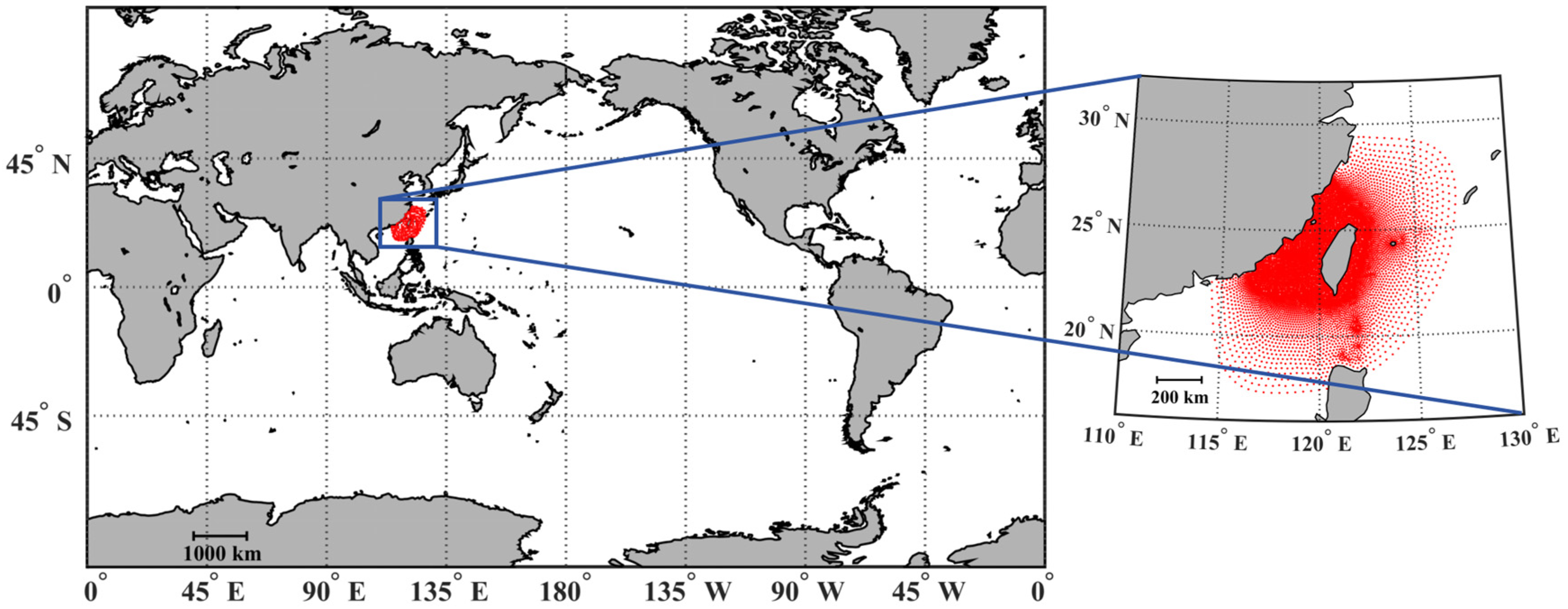
2.1. Data

The data used in this study are obtained from numerical simulations using the SCHISM v5.8.0. The Semi-implicit Cross-scale Hydroscience Integrated System Model (SCHISM, https://ccrm.vims.edu/schismweb/, accessed on 22 March 2025) is a three-dimensional, seamless cross-scale ocean and hydrodynamic numerical model based on an unstructured grid. It was developed from the original SELFE model and has been integrated with multiple physical and biogeochemical modules, including ocean waves, oil spills, water quality, ecosystem dynamics, and turbulence. The model has been successfully applied to various oceanic phenomena, such as storm surges and sediment transport. SCHISM employs a semi-implicit finite element/finite volume method combined with the Euler–Lagrange algorithm to solve the hydrostatic form of the Navier–Stokes equations. This discretization method reduces the Courant–Friedrichs–Lewy (CFL) constraint. Its numerical scheme, which integrates high-order and low-order methods, ensures computational accuracy while maintaining efficiency, enabling it to efficiently and accurately simulate ocean dynamics and ecological processes. Regarding grid design, SCHISM utilizes an unstructured hybrid triangular/quadrilateral grid in the horizontal direction, which can not only adapt to complex coastline terrain but also perform local grid encryption in key areas to effectively balance the computational accuracy and computational complexity. In the vertical direction, the model supports hybrid SZ and LSC2 coordinate systems, enhancing its capability to accurately simulate complex topographic variations. The control equation of SCHISM is as follows [30]:

Momentum equation:

$${\displaystyle \frac{Du}{Dt}}={\displaystyle \frac{\partial }{\partial z}}(\nu {\displaystyle \frac{\partial u}{\partial z}})-g\nabla \eta +f$$

(1)

where u is the horizontal velocity, t is the time, D/Dt represents material derivative (it describes the rate of change of a variable of a fluid element over time), z is the vertical coordinate, $\nu$ is the vertical eddy viscosity coefficient, g is the gravitational acceleration, η is the free surface height, and f represents other forcing terms in the momentum (baroclinic gradient, horizontal viscosity, Coriolis force, tidal potential, atmospheric pressure, and radiation stress).

The depth-integrated form of the continuity equation is as follows:

$$\nabla \cdot u+{\displaystyle \frac{\partial w}{\partial z}}=0$$

(2)

$${\displaystyle \frac{\partial \eta }{\partial t}}+\nabla \cdot {\displaystyle {\int }_{-h}^{\eta }udz}=0$$

(3)

where w is the vertical velocity and h is the water depth.

The tidal potentials of SCHISM’s semi-diurnal tides (M2, S2, N2, K2) are as follows:

$$\widehat{\psi }(\varphi ,\lambda ,t)=C{f}_2{\cos }^2\varphi \cos ({\displaystyle \frac{2\pi t}{T}}+2\lambda +v)$$

(4)

The tidal potentials of SCHISM’s diurnal tides (K1, O1, P1, Q1) are as follows:

$$\widehat{\psi }(\varphi ,\lambda ,t)=C{f}_2{\sin }^2\varphi \cos ({\displaystyle \frac{2\pi t}{T}}+\lambda +v)$$

(5)

where $\widehat{\psi }$ is the tidal potential, $\varphi$ is the latitude, $\lambda$ is the longitude, C is the amplitude of the tidal component, f₂ is the intersection factor, T is the tidal component period, and v is the tidal delay angle.

The study area, shown in Figure 1, is located along the coast of Fujian Province, China. The simulation domain consists of 70,775 grid nodes, with refined grid resolution applied primarily near the coast of Fujian and around Taiwan Island (Figure 1). The LSC2 coordinate system is used in the vertical direction. The water depth is divided into 30 layers, and the reference depth of the sigma layer is 10 m, meaning that waters shallower than this depth may use a hybrid sigma-Z coordinate system, while deeper regions adopt sigma layers. Bathymetric data are obtained from a fused product of nautical charts and ETOPO1, where nautical chart data are used for nearshore regions and ETOPO1 data are applied to offshore areas. The model simulation starts on 21 May 2014, because of the presence of storm surges during this period. The simulation time step is 300 s. The simulation outputs every 0.5 h with a total forecast duration of 5 days.

2.2. Lightweight Methods

Building upon a detailed performance analysis of the original CPU-based Fortran code of the SCHISM model, this study identifies the computationally intensive Jacobi iterative solver module as a key optimization target. The module is restructured and accelerated for GPU implementation, leveraging the advantages of GPU-based large-scale parallel computing.

The optimization of the Jacobi iteration module employed two commonly used GPU acceleration methods, namely, OpenACC and CUDA. In the comparative experiments of this study (Case 2 in Section 3), the CUDA Fortran method was used to achieve lightweight accelerated parallel processing for the SCHISM model. CUDA uses a kernel-based programming approach, offering greater performance and finer-grained control compared to OpenACC. Through low-level optimization, CUDA allows complete control over thread blocks, memory hierarchy, and synchronization, enabling superior performance. The CUDA method involves writing explicit parallel kernel code that runs on the GPU, requiring modifications to the original Fortran code of the SCHISM model via CUDA interfaces to manage data transfer between the host and GPU. Additionally, OpenACC was used to compare the efficiency of Fortran acceleration methods. OpenACC is a high-level directive-based programming model that simplifies GPU parallel programming by adding directives to Fortran code to offload computational tasks to the GPU without modifying the underlying code. It uses the “$acc” directive to mark the regions of code to be accelerated and allows for incremental parallelization. The approach starts by modifying small parts of the code and gradually adding more directives to test acceleration effects. OpenACC also handles data transfers between the host and GPU automatically. While OpenACC is fast, convenient, and highly portable, it offers limited control over low-level optimizations, making it less flexible for handling complex parallel models. In this study, both methods were applied to the GPU-accelerated version of the SCHISM model, and the acceleration effects of these two methods were tested and compared for grid sizes of 2,560,000, 256,000, 70,775, 25,600, and 2560 grid points.

Building upon the GPU rewriting of the source code, this study also designed the following optimization strategies to further achieve efficient parallel computation:

(1) Grid Point Parallel Distribution: Each grid point in the SCHISM model was assigned to an independent GPU thread for computation, with each thread processing a single grid point. Since the grid structure of the SCHISM model inherently supports parallelism, the data computations for each grid point were independent of each other. This method allowed for the full utilization of the large number of parallel computation units available on the GPU.

(2) Splitting Complex Loops: In the SCHISM model, complex nested loops exist that were traditionally designed for CPU serial execution. These loops were rewritten to fit a structure suitable for GPU parallel execution. By splitting complex loops into several smaller loops, each sub-loop task could be executed in parallel, thus improving overall parallelism and GPU utilization.

(3) Dynamically Adjustable Heterogeneous Domain Decomposition: Based on an in-depth analysis of key configuration parameters such as CPU and GPU accelerator clock frequencies, core counts, cache sizes, memory access overhead, floating-point computing power, PCIe bandwidth, and device memory bandwidth in heterogeneous systems, this study proposed a dynamically adjustable heterogeneous domain decomposition method based on an internal–external partitioning strategy. The core idea of this method was to divide the computational domain into internal and external regions, where the internal region contains dense grid points that fully leveraged the high parallel computational capacity of the GPU for acceleration, while the external region included the edge HALO areas handled by the CPU to take advantage of its flexibility and low-latency characteristics. By dynamically adjusting the ratio of the internal to external regions, this method could adapt to different hardware configurations and computational demands, maximizing the overall performance of the heterogeneous system. Experimental results showed that this strategy not only improved GPU computational utilization but also significantly reduced communication overhead between the CPU and GPU, providing a novel solution for efficient domain decomposition in heterogeneous computing environments.

(4) Comprehensive Optimization Measures: Based on the memory hierarchy and computational architecture of the GPU platform, a multi-dimensional optimization strategy was designed to enhance the numerical computation efficiency of the GPU–SCHISM model, specifically including (a) a memory access alignment optimization, which reorganized data structures to achieve global memory coalescing, such that the memory bandwidth pressure was effectively reduced; (b) design of a vectorized conditional branching mechanism to improve SIMD unit utilization; and (c) development of a loop optimization algorithm based on warp-level unrolling to hide memory access latency by increasing instruction-level parallelism. For performance bottleneck modules in the Jacobi iteration solver—such as nonlinear discrete function calculations, sparse matrix-vector multiplication (SpMV), and sparse matrix decomposition—a GPU-architecture-oriented optimization framework was constructed. This included introducing hierarchical storage access patterns to reduce global memory contention, applying mixed-precision computing strategies to enhance floating-point operation density, and designing asynchronous communication mechanisms based on thread–block cooperation to reduce synchronization overhead.

3. Results

3.1. Software and Hardware Platform

Experiments were conducted on a graphics workstation to validate the accuracy and acceleration rate of the proposed GPU–SCHISM lightweight method. The operating system featured CentOS 7.9.2009, with an AMD EPYC 7542 32-core CPU running at 2.85 GHz, 512 GB of memory, and four NVIDIA RTX 4090 GPUs with 24 GB of device memory each. The software environment consisted of the CUDA 12.3 compiler (nvhpc_2023_2311_Linux_x86_64_cuda_12.3).

3.2. Experimental Design

In this study, three control experiments (Case 1-x) running SCHISM using only CPUs are compared with experiments (Case 2-x) using combined CPUs and GPUs. Case 1 consists of three subcases, each utilizing 1 (Case 1-1), 2 (Case 1-2), or 4 (Case 1-4) CPU cores, serving as the baseline runs. Case 2 utilizes the GPU–SCHISM lightweight acceleration framework proposed in this study, leveraging the powerful computational capabilities of the GPU to replace the CPU for computations; the CPU handles logical control, communication, and calculations in the HALO region to achieve GPU acceleration, as detailed in Section 2.2. Case 2 includes three subcases, each utilizing 1 (Case 2-1), 2 (Case 2-2), or 4 (Case 2-4) GPUs and the same number of CPUs on a single computing node. The simulation duration for all six experiments is set to 5 days, with an iteration time step of 300 s, totaling 1440 iterations. All experiments are conducted with the same initial conditions and physical parameters to ensure the comparability of the simulation results.

3.3. Accuracy Validation

To check the accuracy of the model forecast results after the introduction of the GPU–SCHISM lightweight acceleration framework, the simulation results of Case 2-1 are compared with those of Case 1-1. The forecast results from SCHISM for the Fujian coast at 24:00 on Day 3 and Day 5 in Case 1-1 show that at these two moments, the water levels (Figure 2) are lower in the Taiwan Strait and the southern part of the study area, while the water levels are generally higher to the east of Taiwan Island. Figure 3 shows the water level forecast results of GPU–SCHISM for Case 2-1 at the same time. The simulated water levels from GPU–SCHISM (Figure 3) are highly consistent with those from the original SCHISM model (Figure 2), indicating that the GPU acceleration framework can effectively keep the same accuracy with the results using only CPU.

Figure 4 presents the root mean square error (RMSE) distribution of the water level simulation results from Case 2-1 relative to Case 1-1 over the entire 5-day simulation period, which is calculated using the following formula:

$$error=\sqrt{{\displaystyle \frac{\sum _{i=0}^{n-1}{({swh}_{cpu}-{swh}_{gpu})}^2}{n}}}$$

(6)

where ${swh}_{cpu}$ and ${swh}_{gpu}$ represent the water levels from the original SCHISM model and the GPU–SCHISM model, respectively, and $n$ is the number of results for comparison. In Figure 4, the comparison is performed at each grid point based on the time series of simulated results, with $n$ corresponding to the number of temporal model output.

A logarithmic transformation is applied to the RMSE results in Figure 4 to better visualize the wide RMSE distribution across the entire model domain. The RMSEs (Figure 4) are relatively high in the Taiwan Strait and along the northern coastal areas of the study region, with magnitudes ranging from 10⁻⁷~10⁻⁵ m. In contrast, the RMSEs in the southeastern part of the study area are relatively low, with magnitudes ranging from 10⁻⁹~10⁻⁷ m. One source of these errors is the difference in numerical precision: the NVIDIA RTX 4090 GPU used in this study performs single-precision calculations, whereas the CPU performs double-precision computations. The GPU–SCHISM model employs single-precision arithmetic to optimize computational performance. Although this results in minor differences compared to double-precision CPU computations, the RMSE remains on the order of 10⁻⁶ m. This level of precision is sufficient for short-term storm surge forecasts but may limit accuracy for longer-term simulations or other applications requiring higher precision. Future work will explore mixed-precision or double-precision implementations to enhance numerical stability and accuracy in these contexts. Notably, the magnitude of these errors is significantly smaller than the overall magnitude of the simulated water levels. This indicates that GPU–SCHISM maintains nearly the same computational accuracy as the original CPU-based SCHISM model, further validating the accuracy of the lightweight GPU acceleration framework within the SCHISM model and its feasibility for short-term simulations (less than one week).

To further validate the accuracy of GPU–SCHISM, the RMSEs of water level predictions across the entire model domain at Day 3, 24:00 and Day 5, 24:00 are computed, yielding values of ${4.08\times 10}^{-4}$ m and ${4.57\times 10}^{-6}$ m (

Table 1. Water levels and their RMSEs in the original SCHISM model experiment (Case 1-1) and GPU–SCHISM experiment (Case 2-1).

Time	Average Water Level from CPU-Based SCHISM (m)	Average Water Level Simulated by GPU–SCHISM (m)	RMSE Between CPU-Based SCHISM and GPU–SCHISM (m)
Day 3, 24:00	0.3714	0.3714	4.08 × 10−4
Day 5, 24:00	0.0294	0.0294	4.57 × 10−6

), respectively. The regions with higher RMSEs are primarily located near the coastline. This result shows that the mean absolute errors of the two models at all spatial nodes are strictly controlled under the order of ${1.0\times 10}^{-4}$ m. It can be considered that the calculation results of GPU–SCHISM are consistent with those of the original SCHISM. For 24:00 on Day 5, dimensional analysis is based on the water level physical unit system (meter). When expressed in scientific notation, the error magnitude of ${4.57\times 10}^{-6}$ m means that the calculation results of the two models remain completely consistent at the fifth decimal place (corresponding to the 10⁻⁵ m level) and only differ at the sixth place (10⁻⁶ m level). This error magnitude is four orders of magnitude lower than the centimeter-level accuracy (10⁻² m) required for hydrological forecasting. In addition, the error magnitude at Day 3, 24:00 is two orders of magnitude lower than the centimeter-level accuracy required for hydrological forecasting. This scale difference can be regarded as calculation consistency in engineering practice, which fully confirms the reliability of the GPU-accelerated model at the physical forecasting level.

3.4. Lightweight Acceleration Performance

To evaluate the acceleration performance of a single-node GPU, the runtime comparisons between the original CPU-based SCHISM experiments and the GPU–SCHISM experiments over the 5-day forecast period are shown in Figure 5. For the Jacobi iterative solver module optimized in this study, using a single GPU yields a significant speedup with a runtime of 236.8 s, which is substantially lower than the 725.5 s using a single CPU core, resulting in a speedup ratio of 3.06. This demonstrates a clear computational advantage of the GPU in this scenario. As the number of CPU cores increases, the runtime of the CPU-based SCHISM experiments gradually decrease from 725.5 s with a single core to 224.5 s with four cores. However, in the GPU–SCHISM experiments, increasing the number of GPUs does not yield the expected acceleration. The runtime with two GPUs is comparable to that with two CPU cores, while the runtime with four GPUs is significantly longer than that of the four-core CPU case.

Increases in the numbers of both CPU cores and GPUs generally reduce computational runtime. However, the rate of reduction is slower in the GPU–SCHISM experiments. Using a single GPU reduces the runtime by 414.4 s compared to the single-core CPU, demonstrating good acceleration capability. However, with two GPUs, the runtime is similar to that of the two-core CPU, and with four GPUs, the runtime not only fails to show further acceleration but even exceeds that of the four-core CPU.

Figure 6 shows the speedup ratio of the GPU–SCHISM experiments compared with the CPU version of the SCHISM experiments. The speedup ratio is calculated based on the runtime of the corresponding CPU core number benchmark experiment. The results indicate that, for both the Jacobi iterative solver module and the overall model runtime, a single GPU provides the best acceleration, achieving speedup ratios of 3.06 and 1.18, respectively. The speedup of GPU–SCHISM is moderate compared to the acceleration effects of the other atmosphere and ocean models in

Table 2. Existing GPU porting work in climate fields. The speedups are normalized to one CPU core.

Model Name	Model Description	Porting Modules to GPU	Speedup
WRF	Weather Research and Forecasting	WSM5 microphysics	8
WRF-Chem	WRF Chemical	Chemical kinetics kernel	8.5
POP	Parallel Ocean Program	Loop structures	2.2
POM	Princeton Ocean Model	POM.gpu code	6.8
GPU–SCHISM	GPU-Semi-implicit Cross-scale Hydroscience Integrated System Model	Jacobian iterative solver module	3.06

. However, as the number of GPUs increases, the acceleration efficiency declines instead of improving. In particular, with four GPUs, the computational efficiency is even lower than that of the corresponding CPU experiments, indicating that GPU parallel scalability is limited under the current computational framework.

This experiment reveals an anomalous acceleration characteristic of GPU–SCHISM in Case 2 (grid size: 70,775). Specifically, as the number of GPU accelerators increases from one to four, the computational performance does not achieve the expected linear scaling; instead, the efficiency declines.

The scalability limitations of the multi-GPU implementation arise from a reduction in computational workload per GPU as the number of GPUs increases. This reduces the parallel efficiency of each device and increases the relative impact of communication overhead. We profile the communication overhead using NVIDIA Nsight Systems. Profiling results show that PCIe communication latency contributes to this bottleneck, particularly in the absence of overlapping communication with computation. Results indicate a PCIe communication latency of approximately 1.2 ms per data exchange, with effective bandwidth utilization of around 7.5 GB/s. The increased number of GPUs lead to reduced workload per device and elevated inter-GPU communication frequency, resulting in significant synchronization delays. Consequently, under the current architecture and PCIe-based communication, the scalability of GPU–SCHISM is constrained, particularly for small- to medium-grid resolutions.

Since GPUs generally demonstrate greater advantages in large-scale numerical simulations, their acceleration performance may depend on the number of grid points in the simulation domain. To further analyze the relationship between grid resolution and GPU performance, we perform tests on a simplified computational kernel based on the Jacobi iterative solver. The results indicate that CUDA Fortran achieves substantial speedup for large grid sizes, particularly when the number of grid points exceeds 256,000. In contrast, for small grid sizes, GPU acceleration provides limited benefits due to the underutilization of hardware resources and higher communication overhead. A comparison with OpenACC shows that although it also offers acceleration, its performance is consistently lower than that of CUDA Fortran across all grid resolutions tested. Therefore, Figure 7 presents the runtimes and speedup ratios of CPU and GPU calculations under different grid resolutions. Additionally, since there are two methods for GPU acceleration using CUDA Fortran and OpenACC, in order to further compare the performance of different acceleration methods, Figure 7 also includes the results using the OpenACC acceleration method. As shown in the figure, when the number of grid points is reduced from 2,560,000 to 256,000, the GPU runtime (for both CUDA and OpenACC) decreases substantially, similar to the CPU runtime. However, when the number of grid points is less than 256,000, the GPU runtimes do not decrease significantly with the grid size. Specifically, when the number of grid points is set to 2,560,000, 256,000, and 70,775, CUDA Fortran shows good acceleration effects, with speedup ratios of 35.13, 4.21, and 1.27 respectively. However, when the number of grid points is further reduced to 25,600 and below, CUDA Fortran actually reduces the computational efficiency, which is the main reason why the runtime of the system with 4 GPUs is longer than that of the system with 4 CPUs, as mentioned above. When the subdomain grid size per GPU increases, its computationally intensive nature allows streaming multiprocessors (SMs) to sustain a higher number of active threads, thereby maintaining a continuous computational load, significantly improving memory bandwidth utilization, and fully leveraging GPU computational capabilities. This finding suggests that CPUs are more efficient for small-scale grid simulations than GPUs, while GPUs exhibit significant advantages in large data simulations.

Furthermore, the OpenACC GPU acceleration method demonstrates a performance boost for grid sizes of 2,560,000 and 256,000, with a speedup trend similar to that of CUDA, i.e., decreasing speedup as the number of grid points reduces. However, it is noteworthy that the speedup achieved by OpenACC remains consistently lower than that achieved by CUDA, indicating that CUDA provides superior acceleration performance to the OpenACC in this study.

In terms of power consumption and energy efficiency, this paper utilizes the NVIDIA RTX 4090 24 GB GPU, which boasts a theoretical single-precision floating-point performance of 82.58 TFLOPS and a thermal design power (TDP) of 450 W, alongside the AMD EPYC 7542 32-core CPU, which has a theoretical single-precision floating point performance of 3.48 TFLOPS and a TDP of 225 W. From these numbers, it can be deduced that the NVIDIA RTX 4090 24 GB GPU’s floating-point performance is 23.7 times that of the AMD EPYC 7542 32-core CPU. Although the NVIDIA RTX 4090 24 GB GPU’s TDP is twice that of the AMD EPYC 7542 32-core CPU, it offers 23.7 times the computational power, indicating that the GPU used in this study theoretically has a higher “energy efficiency ratio”. On the other hand, the actual test data for the speedup ratio, shown in Figure 7 of this paper, reveals a speedup ratio of 35.13 at 256,000 grid points. This demonstrates that, despite consuming seven times the power of the CPU (using four GPUs), a speedup ratio of 35.13 is achieved, indicating that the “energy efficiency ratio” is superior to that of a CPU-only acceleration approach.

4. Conclusions and Discussion

To enhance the computational efficiency of the SCHISM model, this study developed a GPU-accelerated version, GPU–SCHISM, based on the CUDA Fortran approach and evaluated its performance in single-node GPU acceleration. Analysis of a series of numerical simulation experiments yielded the following key conclusions:

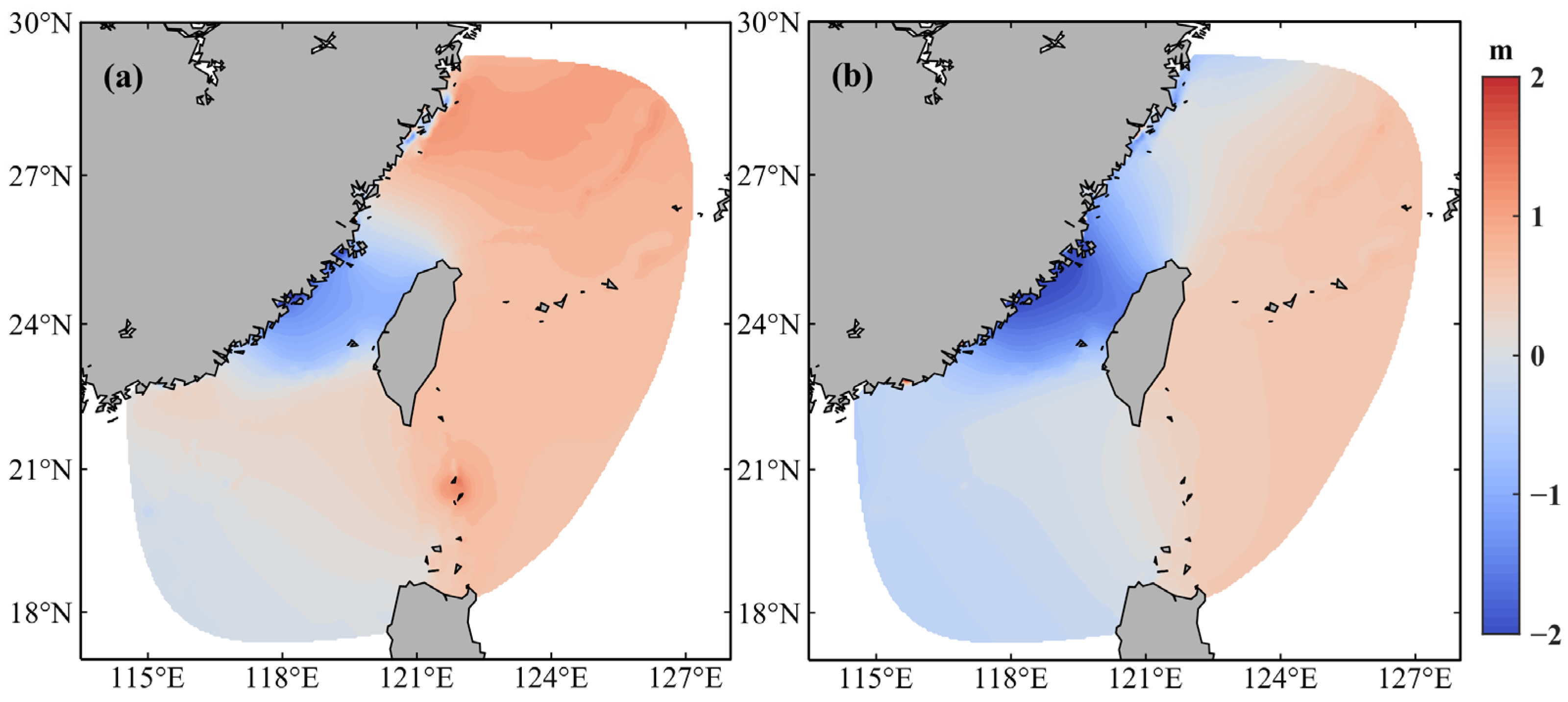
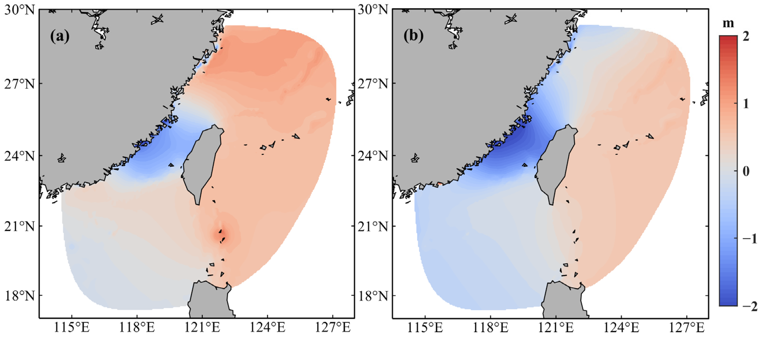
• The GPU–SCHISM model is able to maintain the accuracy as the simulation results by utilizing only CPU. The error in the water level simulation between the accelerated GPU version and the original CPU version is less than 10⁻⁶ m.
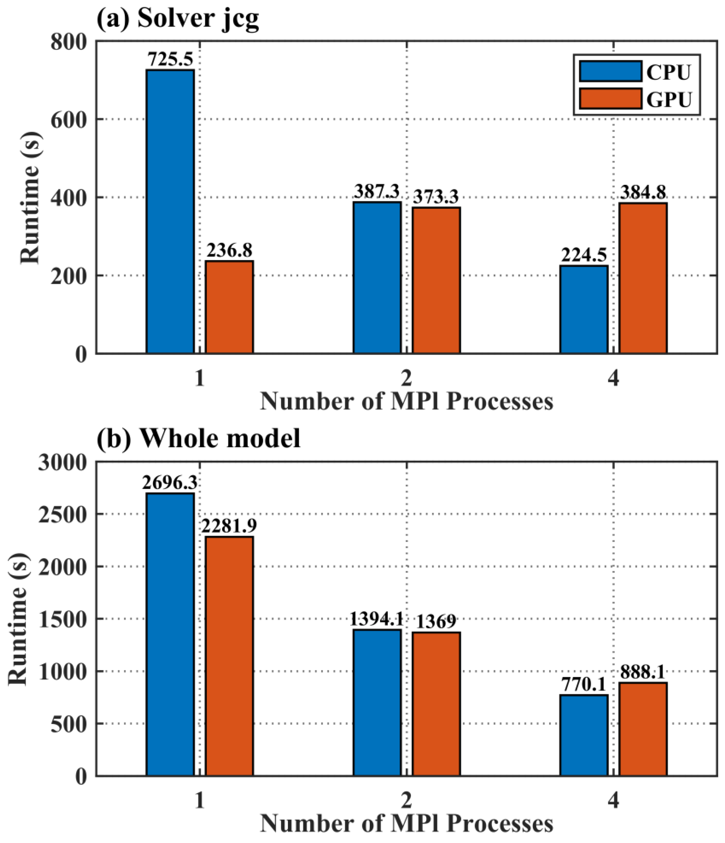
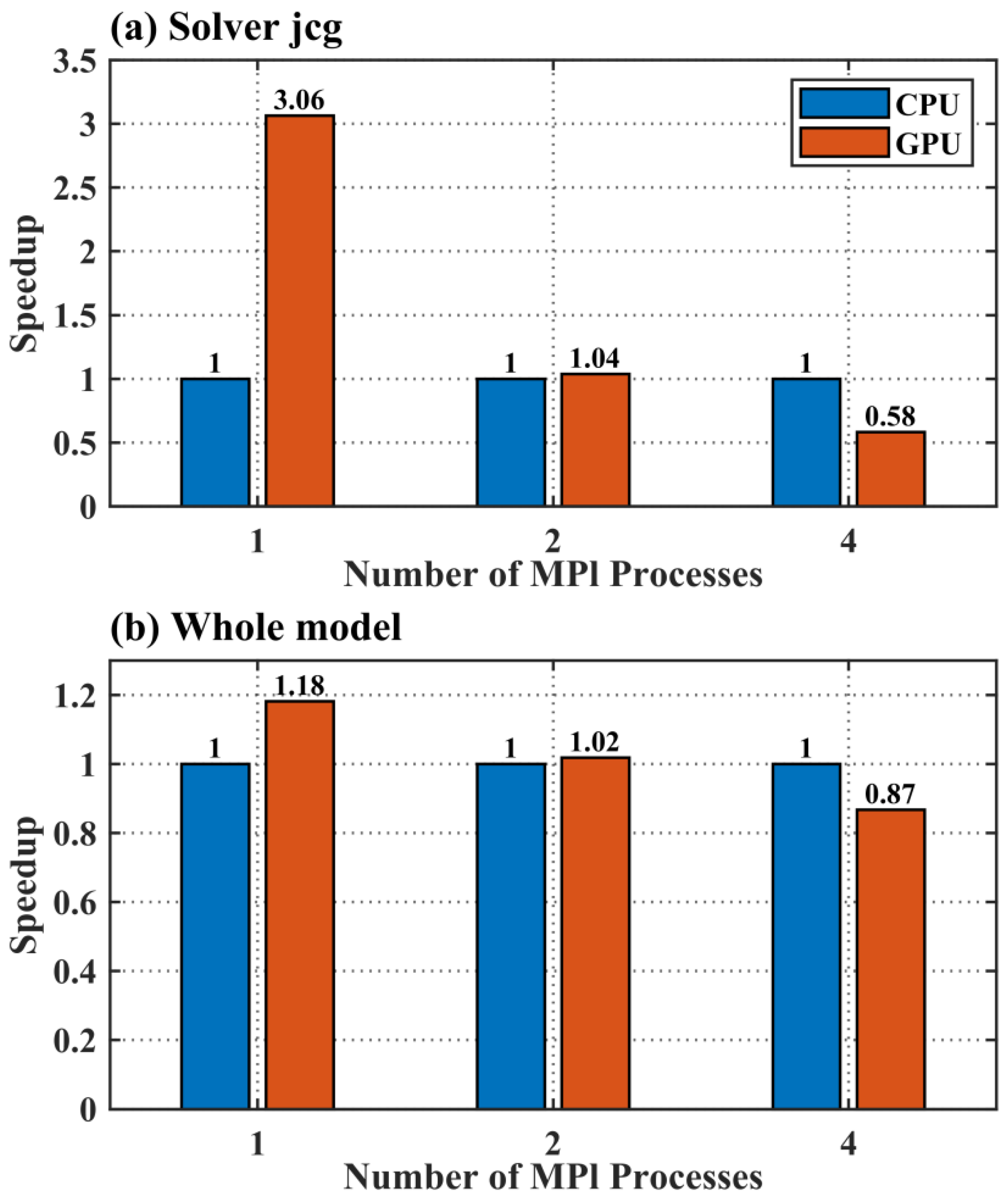
• The model using single GPU exhibits significant acceleration effects. The Jacobian iterative solver module, when accelerated with one GPU, completes a five-day water level forecast in 236.8 s, achieving a speedup ratio of 3.06, differing from that of a single-core CPU. The entire GPU–SCHISM model completes the five-day forecast in 2281.9 s, with an overall speedup ratio of 1.18.
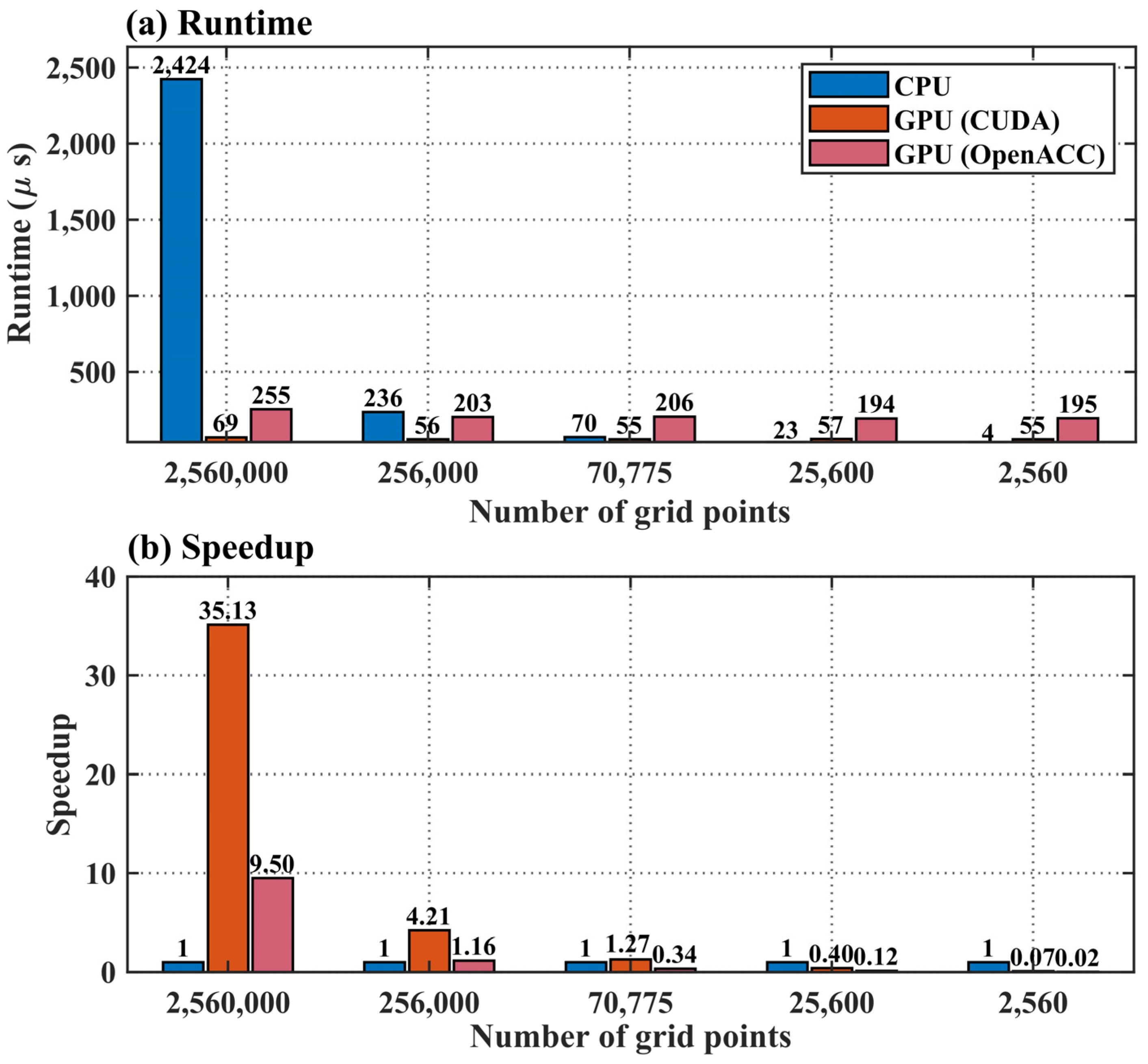
• The parallel expansion acceleration of GPU depends on the scale of calculation. In high-resolution, large-scale calculations, GPU has a significant advantage, with a GPU speedup ratio of 35.13 with 2,560,000 grid points; in small-scale calculations, the GPU calculation efficiency is lower than that of CPU.
• A comparison between the two Fortran-based GPU acceleration approaches, CUDA and OpenACC, reveals that the CUDA method employed in this study provides superior acceleration performance.

This study is the first attempt to implement GPU acceleration of the SCHISM model under the CUDA Fortran framework. For small-scale simulations, GPU–SCHISM exhibits limited acceleration benefits. In these cases, the insufficient parallel workload leads to the underutilization of GPU computational resources, while data transfer and synchronization overheads become relatively more significant. Therefore, CPU-based computing remains preferable for low-resolution or small-domain simulations. The results preliminarily verify the acceleration potential of GPU–SCHISM in high-resolution numerical simulations. Several aspects for optimization can be explored in future studies. First, based on our experiments results that indicate that a single GPU offers significant acceleration, future research can focus on optimizing GPU task allocation strategies and identifying key computational modules for acceleration to enhance the overall computational efficiency of the SCHISM model. Second, more optimization strategies can be adopted during the recoding of the source code for the GPU. For example, data preloading and asynchronous transmission can be adopted. Constant data over time can be uploaded to the GPU device memory at once, avoiding frequent data transmission between the CPU and GPU during the calculation process, thereby reducing communication delays. In addition, boundary data required for the next time step can be preloaded while computing the current time step, effectively overlapping data transfer with computation. This approach reduces overall GPU idle time and data communication overhead, ultimately providing a more efficient and lightweight computational tool for high-resolution oceanic numerical simulations.

References

- Feng, X.; Li, M.; Li, Y.; Yu, F.; Yang, D.; Gao, G.; Xu, L.; Yin, B. Typhoon storm surge in the southeast Chinese mainland modulated by ENSO. Sci. Rep. 2021, 11, 10137. [Google Scholar] [CrossRef]
- Wang, K.; Yang, Y.; Reniers, G.; Huang, Q. A study into the spatiotemporal distribution of typhoon storm surge disasters in China. Nat. Hazards 2021, 108, 1237–1256. [Google Scholar]
- Glahn, B.; Taylor, A.; Kurkowski, N.; Shaffer, W.A. The role of the SLOSH model in National Weather Service storm surge forecasting. Natl. Weather. Dig. 2009, 33, 3–14. [Google Scholar]
- Kohno, N.; Dube, S.K.; Entel, M.; Fakhruddin, S.H.M.; Greenslade, D.; Leroux, M.; Rhome, J.; Thuy, N.B. Recent progress in storm surge forecasting. Trop. Cyclone Res. Rev. 2018, 7, 55–66. [Google Scholar] [CrossRef]
- Luettich, R.A.; Westerink, J.J. Formulation and Numerical Implementation of the 2D/3D ADCIRC Finite Element Model Version 44; University of North Carolina: Chapel Hill, NC, USA, 2004. [Google Scholar]
- Chen, C.; Beardsley, R.C.; Cowles, G. An Unstructured Grid, Finite-Volume Coastal Ocean Model (FVCOM) System. Oceanography 2006, 19, 78–89. [Google Scholar] [CrossRef]
- Zhang, Y.; Baptista, A.M. SELFE: A semi-implicit Eulerian–Lagrangian finite-element model for cross-scale ocean circulation. Ocean Model. 2008, 21, 71–96. [Google Scholar] [CrossRef]
- Yin, B.-S.; Hou, Y.-J.; Cheng, M.-H.; Su, J.-Z.; Lin, M.-X.; Li, M.-K.; El-Sabh, M.I. Numerical study of the influence of waves and tide-surge interaction on tide-surges in the Bohai Sea. Chin. J. Oceanol. Limnol. 2001, 19, 97–102. [Google Scholar]
- Dietrich, J.C.; Zijlema, M.; Westerink, J.J.; Holthuijsen, L.H.; Dawson, C.; Luettich, R.A.; Jensen, R.E.; Smith, J.M.; Stelling, G.S.; Stone, G.W. Modeling hurricane waves and storm surge using integrally-coupled, scalable computations. Coast. Eng. 2011, 58, 45–65. [Google Scholar]
- Feng, X.; Sun, J.; Yang, D.; Yin, B.; Gao, G.; Wan, W. Effect of Drag Coefficient Parameterizations on Air–Sea Coupled Simulations: A Case Study for Typhoons Haima and Nida in 2016. J. Atmos. Ocean. Technol. 2021, 38, 977–993. [Google Scholar] [CrossRef]
- Feng, X.; Yin, B.; Yang, D. Development of an unstructured-grid wave-current coupled model and its application. Ocean Model. 2016, 104, 213–225. [Google Scholar] [CrossRef]
- Li, S. On the consistent parametric description of the wave age dependence of the sea surface roughness. J. Phys. Oceanogr. 2023, 53, 2281–2290. [Google Scholar] [CrossRef]
- Häfner, D.; Nuterman, R.; Jochum, M. Fast, cheap, and turbulent-global ocean modeling with GPU acceleration in Python. J. Adv. Model. Earth Syst. 2021, 13, e2021MS002717. [Google Scholar]
- Yuan, Y.; Yang, H.; Yu, F.; Gao, Y.; Li, B.; Xing, C. A wave-resolving modeling study of rip current variability, rip hazard, and swimmer escape strategies on an embayed beach. Nat. Hazards Earth Syst. Sci. 2023, 23, 3487–3507. [Google Scholar]
- Ikuyajolu, O.J.; Van Roekel, L.; Brus, S.R.; Thomas, E.E.; Deng, Y.; Sreepathi, S. Porting the WAVEWATCH III (v6.07) wave action source terms to GPU. Geosci. Model Dev. Discuss. 2023, 16, 1445–1458. [Google Scholar]
- Xu, S.; Huang, X.; Oey, L.-Y.; Xu, F.; Fu, H.; Zhang, Y.; Yang, G. POM.gpu-v1.0: A GPU-based princeton ocean model. Geosci. Model Dev. 2015, 8, 2815–2827. [Google Scholar] [CrossRef]
- Qin, X.; LeVeque, R.J.; Motley, M.R. Accelerating an adaptive mesh refinement code for depth-averaged flows using graphics processing units (GPUs). J. Adv. Model. Earth Syst. 2019, 11, 2606–2628. [Google Scholar]
- Jiang, J.; Lin, P.; Wang, J.; Liu, H.; Chi, X.; Hao, H.; Wang, Y.; Wang, W.; Zhang, L. Porting LASG/IAP Climate System Ocean Model to Gpus Using OpenAcc. IEEE Access 2019, 7, 154490–154501. [Google Scholar] [CrossRef]
- Brodtkorb, A.R.; Holm, H.H. Coastal ocean forecasting on the GPU using a two-dimensional finite-volume scheme. Tellus A Dyn. Meteorol. Oceanogr. 2021, 73, 1–22. [Google Scholar]
- Yuan, Y.; Yu, F.; Chen, Z.; Li, X.; Hou, F.; Gao, Y.; Gao, Z.; Pang, R. Towards a real-time modeling of global ocean waves by the fully GPU-accelerated spectral wave model WAM6-GPU v1.0. Geosci. Model Dev. 2024, 17, 6123–6136. [Google Scholar]
- Jablin, T.B.; Prabhu, P.; Jablin, J.A.; Johnson, N.P.; Beard, S.R.; August, D.I. Automatic CPU-GPU communication management and optimization. In Proceedings of the 32nd ACM SIGPLAN Conference on Programming Language Design and Implementation, San Jose, CA, USA, 4–8 June 2011; pp. 142–151. [Google Scholar]
- Mittal, S.; Vaishay, S. A survey of techniques for optimizing deep learning on GPUs. J. Syst. Arch. 2019, 99, 101635. [Google Scholar]
- Sharkawi, S.S.; Chochia, G.A. Communication protocol optimization for enhanced GPU performance. IBM J. Res. Dev. 2020, 64, 9:1–9:9. [Google Scholar]
- Hopkins, M.; Mikaitis, M.; Lester, D.R.; Furber, S. Stochastic rounding and reduced-precision fixed-point arithmetic for solving neural ordinary differential equations. Philos. Trans. R. Soc. Lond. Ser. A 2020, 378, 20190052. [Google Scholar]
- Gupta, R.R.; Ranga, V. Comparative study of different reduced precision techniques in deep neural network. In Proceedings of the International Conference on Big Data, Machine Learning and their Applications, Prayagraj, India, 29–31 May 2020; Tiwari, S., Suryani, E., Ng, A.K., Mishra, K.K., Singh, N., Eds.; Springer: Singapore, 2021; pp. 123–136. [Google Scholar]
- Rehm, F.; Vallecorsa, S.; Saletore, V.; Pabst, H.; Chaibi, A.; Codreanu, V.; Borras, K.; Krücker, D. Reduced precision strategies for deep learning: A high energy physics generative adversarial network use case. arXiv 2021, arXiv:2103.10142. [Google Scholar]
- Noune, B.; Jones, P.; Justus, D.; Masters, D.; Luschi, C. 8-bit numerical formats for deep neural networks. arXiv 2022, arXiv:2206.02915. [Google Scholar]
- TensorFlow Accelerating AI Performance on 3rd Gen Intel Xeon Scalable Processors with TensorFlow and Bfloat16, 2020. Available online: https://blog.tensorflow.org/2020/06/accelerating-ai-performance-on-3rd-gen-processors-with-tensorflow-bfloat16.html (accessed on 18 June 2021).
- Tintó Prims, O.; Acosta, M.C.; Moore, A.M.; Castrillo, M.; Serradell, K.; Cortés, A.; Doblas-Reyes, F.J. How to use mixed precision in ocean models: Exploring a potential reduction of numerical precision in NEMO 4.0 and ROMS 3.6. Geosci. Model Dev. 2019, 12, 3135–3148. [Google Scholar]
- Zhang, Y.J.; Ye, F.; Stanev, E.V.; Grashorn, S. Seamless cross-scale modeling with SCHISM. Ocean Model. 2016, 102, 64–81. [Google Scholar]