Abstract
Accurate shoreline extraction is critical for coastal engineering applications, including erosion monitoring, disaster response, and sustainable management of island ecosystems. However, traditional methods face challenges in large-scale monitoring due to high costs, environmental interference (e.g., cloud cover), and poor performance in complex terrains (e.g., bedrock coastlines). This study developed an optimized DeepLabV3+ model for the extraction of island shorelines, which improved model performance by replacing the backbone network with MobileNetV2, introducing a strip pooling layer into the ASPP module, and adding CBAM modules in both the shallow and deep stages of feature extraction from the backbone network. The model accuracy was verified using a self-built drone dataset of the shoreline of Koh Lan, Thailand, and the results showed: (1) Compared with the control model, the improved DeepLabV3+ model performs excellently in pixel accuracy (PA), recall, F1 score, and intersection over union (IoU), reaching 98.7%, 97.7%, 98.0%, and 96.2%, respectively. Meanwhile, the model has the lowest number of parameters and floating-point operations, at 6.61 M and 6.7 GFLOPS, respectively. (2) In terms of pixel accuracy (PA) and intersection over union (IoU), the CBAM attention mechanism outperforms the SE-Net and CA attention mechanisms. Compared with the original DeepLabV3+ network, PA increased by 3.1%, and IoU increased by 8.2%. (3) The verification results of different types of coastlines indicate that the improved model can effectively distinguish between shadows and water bodies, reducing the occurrence of false negatives and false positives, thereby lowering the risk of misclassification and obtaining better extraction results. This work provides a cost-effective tool for dynamic coastal management, particularly in data-scarce island regions.
1. Introduction
Shoreline refers to the boundary line where a body of water, such as an ocean, lake, or river, meets the land [1]. Shoreline survey [2] and extraction are crucial for ecological conservation [3] as well as coastal planning [4], and disaster prevention, as they can reveal the ecological conditions of the coast, identify erosion and sedimentation [5], and guide the rational planning of coastal resources. Furthermore, shoreline change data lay the foundation for geomorphological and dynamic studies, enhance understanding of coastal evolution, and provide scientific support for dealing with natural disasters [6,7] and climate change [8].
1.1. Shoreline Measurement: Traditional Limitations and Remote Sensing Innovations
Traditional shoreline measurement techniques, such as plane surveying, tidal staff method, and hydrographic surveying [9], are limited by time-consuming and labor-intensive processes as well as the cost of building hydrological stations, especially in remote and rugged island areas where various difficulties are often encountered. To automate the analysis of shoreline change rates derived from historical data, tools such as the Digital Shoreline Analysis System (DSAS) [10] have been developed. DSAS employs statistical methods to quantify shoreline movement over time, supporting coastal erosion and accretion studies. However, its dependency on manually digitized shoreline data still limits scalability in large-scale or high-resolution monitoring. The continuous advancement of remote sensing technology has brought revolutionary changes to shoreline detection [11]. The shoreline extracted through remote sensing is often referred to, in a strict sense, as the Remote Sensing Shoreline or the Instantaneous Waterline [12]. This shoreline is the position of the coastline captured at a specific time through satellite remote sensing and low-altitude remote sensing technology from unmanned aerial vehicles [13,14], typically representing the boundary between water and land at the instant of image acquisition. Compared to satellite remote sensing, unmanned aerial vehicle (UAV) low-altitude remote sensing technology [15] offers greater flexibility and mobility, not being constrained by satellite revisit cycles. The ultra-low-altitude flight capability of drones enables them to bypass atmospheric cloud interference, rapidly acquiring small-scale, high-resolution imagery of islands. This provides an effective technical means for the refined mapping of island shorelines and for responding to short-term coastal changes and emergency responses such as flood warnings.
With the rapid development of geographic information science [16,17] and remote sensing technology [18], shoreline extraction technology has become a hot research area. From the late 20th century to the early 21st century, this process mainly relied on a series of classic image processing techniques, each with its unique application scenarios and challenges. The advantages and disadvantages of several mainstream image processing techniques in shoreline extraction are shown in Table 1.

Table 1.
Technical Analysis and Evaluation of Traditional Coastal Line Extraction.
With the increasing availability of high-resolution data sources and the continuous improvement of spatial resolution, traditional shoreline extraction methods such as image segmentation and edge detection show significant limitations when dealing with complex terrains and high-resolution demands [26]. These methods struggle to adapt to shoreline feature variability and often require manual parameter adjustments, hindering full automation and limiting their applicability in large-scale shoreline change monitoring [27].
1.2. Artificial Intelligence Algorithms Empower Remote Sensing Shoreline Extraction
In recent years, deep learning, as a significant branch of machine learning, has achieved rapid development. In particular, Convolutional Neural Networks (CNNs) have made groundbreaking progress in various fields such as image classification [28,29], object detection [30,31], and semantic segmentation [32], thanks to their exceptional feature extraction capabilities. In the task of shoreline extraction, deep learning algorithms leverage their strong generalization and multi-dimensional information fusion capabilities to achieve high-precision shoreline extraction. Their abilities in automatic threshold segmentation and automatic feature extraction offer new possibilities for the automated extraction of shorelines.
For instance, Dang et al. [33] effectively employed the U-Net model to assess the shoreline and coastline recognition due to coastal erosion caused by sea-level rise from storm events over 20 years in Vietnam. Scala et al. [34] developed a U-Net-based semantic segmentation method for shoreline extraction from aerial/satellite images, achieving 85% accuracy and 80% IoU using the Coast Train dataset. The model effectively distinguished water from land and other categories, demonstrating high precision in coastline detection in Sicily, Italy. Feng et al. [35] proposed the CSAFNet model, which, by integrating edge depth supervision and attention fusion mechanisms, significantly enhanced the precision of shoreline segmentation from satellite remote sensing imagery. Aryal et al. [36] proposed a modified U-Net variant that, using sparsely labeled data, automated the mapping of 4-band NOAA imagery, achieving an IoU of 94.86%, comparable to traditional ML methods (95.05% IoU), thus supporting Arctic shoreline mapping.
However, mainstream deep-learning network models for shoreline extraction are currently confronted with numerous challenges. On the one hand, these models typically contain a large number of parameters, which not only leads to high computational costs during model training and inference but also increases the storage requirements of the models. On the other hand, the floating-point operations (FLOPs) of these models are extremely high, further exacerbating the computational burden. This high computational complexity makes it difficult to achieve efficient operation while ensuring the accuracy of shoreline extraction, thereby posing obstacles to the real-time automated management of shorelines. Particularly in resource-constrained environments, such as UAV platforms or embedded devices, the high computational demands of these models limit their practical application. Therefore, how to optimize the computational efficiency of the models without sacrificing extraction accuracy is a pressing issue that needs to be addressed in the field of shoreline extraction [37].
DeepLabV3+ [38] is a deep learning model for image semantic segmentation proposed by Google’s research team in 2018. This model builds upon the multi-scale context information extraction technology of its predecessor, DeepLabV3, incorporates an Encoder-Decoder architecture and introduces Atrous Separable Convolution (also known as Dilated Convolution). This allows the network to perceive both small details and large-scale structures in the image simultaneously, enhancing the precision of segmentation boundaries while maintaining high spatial resolution. Although DeepLabV3+ has demonstrated exceptional performance in the field of image segmentation, it still faces challenges when dealing with shorelines that have complex features, such as blurred boundaries and discontinuous segmentation. Furthermore, the high parameter counts of its backbone network and relatively low operational efficiency limit the model’s flexibility in applications on mobile platforms.
To overcome the aforementioned issues, this paper proposes a lightweight shoreline extraction method based on an improved DeepLabV3+ network. By replacing the Xception [39] in the backbone network with MobileNetV2 [40], and introducing the Strip Pooling layer [41] and CBAM attention mechanism (Convolutional Block Attention Module) [42], the method aims to optimize the precision of shoreline extraction and enhance the operational efficiency of the extraction process. To comprehensively evaluate the performance of the improved DeepLabV3+ in land-sea segmentation capabilities, this study conducts experiments based on the drone dataset of Koh Lan, Thailand, and compares and analyzes it with FCN8 [43], SegNet [44], U-Net [45], and the original DeepLabV3+ model. The aim of the research is to verify the application potential of the improved DeepLabV3+ in the field of shoreline extraction, providing an efficient and accurate technical means for dynamic shoreline monitoring and marine resource management. The main contributions of this paper can be summarized as follows:
- (1)
- In response to the challenges of feature extraction in complex coastal environments, this study innovatively integrates a Strip Pooling layer and CBAM dual-attention modules into the DeepLabV3+ model, constructing a network architecture capable of perceiving multi-scale contextual information. The Strip Pooling layer enables the model to effectively capture long-range spatial dependencies of shorelines, while the CBAM channel-spatial attention mechanism dynamically enhances key features. This combination improves the model’s ability to identify fragmented shorelines and areas with blurred textures. Tested on a drone dataset from Koh Lan Island, Thailand, the model achieved a pixel accuracy (PA) of 98.7% and an intersection over union (IoU) of 96.2%, surpassing classic models such as U-Net, FCN8, SegNet, and the original DeepLabV3+ model. This achievement offers a novel solution for shoreline extraction from high-resolution remote sensing imagery.
- (2)
- To address the issue of low computational efficiency in traditional deep learning models, we redesigned the backbone network of DeepLabV3+ by replacing Xception with MobileNetV2 and incorporating depthwise separable convolutions. This optimization reduced the number of parameters by 88% and the floating-point operations (FLOPs) by 67%, enabling real-time processing on UAV platforms. The lightweight design maintains high accuracy while reducing hardware requirements, making it suitable for resource-constrained environments.
- (3)
- The integration of UAVs and deep learning offers a scalable solution for dynamic shoreline monitoring, especially in data-scarce island regions. By automating high-precision shoreline extraction, this framework supports critical applications such as erosion risk assessment, disaster response, and sustainable coastal planning.
2. Materials and Methods
2.1. Study Area and Data Collection
2.1.1. Overview of the Study Area
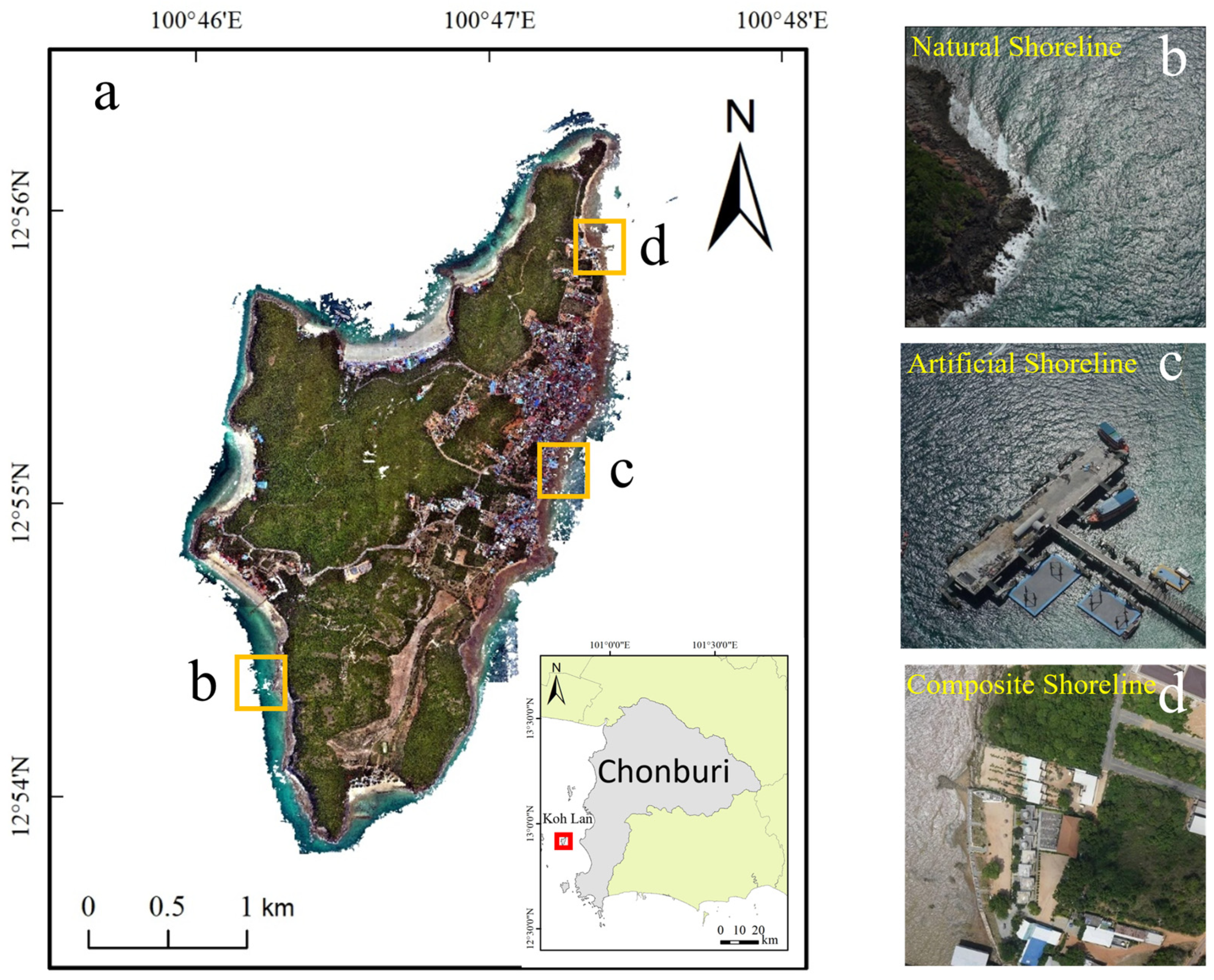
Koh Lan is located near the coast of Chon Buri Province, Thailand (100°45′ E–100°48′ E, 12°53′ N–12°57′ N), with a total area of approximately 6.82 km2. It is a well-known tourist and holiday island in Thailand (as shown in Figure 1a). The coastline of Koh Lan is winding, with different shoreline types varying in length and frequently alternating in space, making it an ideal area for shoreline extraction and verification research.

Figure 1.
Location and illustrations of different shoreline types the study area in Koh Lan, Thailand. (a) Location map of Koh Lan; (b) Natural shoreline; (c) Artificial shoreline; (d) Composite shoreline.
Shorelines are generally classified into two main categories based on their formation causes and characteristics: natural shorelines and artificial shorelines [46]. The artificial shoreline of Koh Lan (Figure 1c) mainly consists of coastlines that have been constructed or modified by human activities, such as docks and seawalls. The natural shoreline of Koh Lan (Figure 1b) can be further divided into three subtypes [47]: Bedrock shorelines, sandy shorelines, and muddy shorelines. Bedrock shorelines are coastlines composed of rocks such as granite, sandstone, or shale. They are characterized by their high stability and resistance to erosion from waves and tides. Sandy shorelines consist of loose particles like sand grains and silt, and they exhibit dynamic changes, being easily influenced by marine dynamics and climate changes. Muddy shorelines are coastlines made up of fine-grained sediments such as mud and clay. They have strong depositional and erosional processes and are often home to mangroves and coastal wetland vegetation. Considering the varying lengths and frequent spatial alternation of different shoreline types on Koh Lan, this study introduces a third type of shoreline the composite shoreline (Figure 1d), which refers to areas where natural and artificial shorelines are interwoven. This classification not only enriches the diversity of shoreline types but also more comprehensively reflects the complexity of shoreline types.
2.1.2. Data Acquisition and Preprocessing
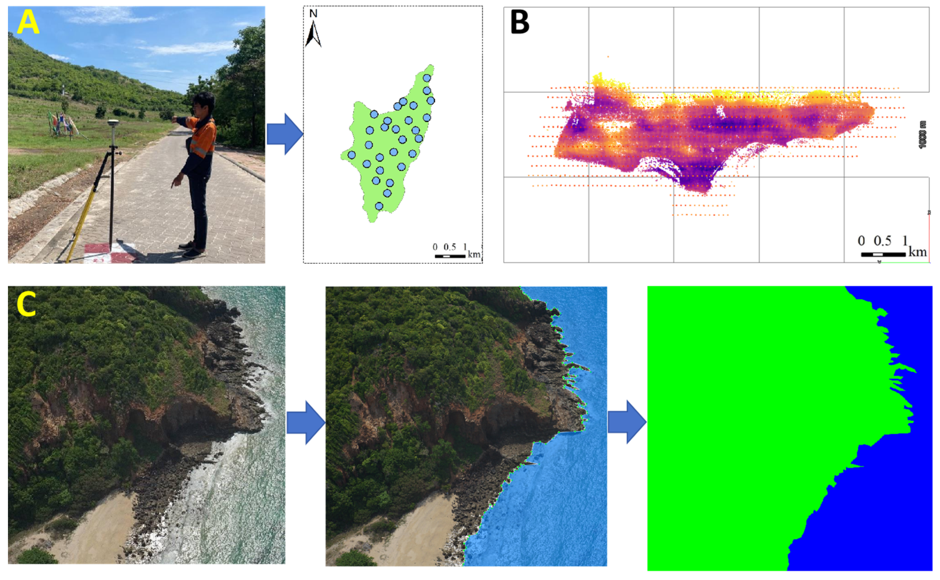
In this study, a CW-15 vertical (Chengdu Zong Heng Unmanned Aerial Vehicle Technology Co., Ltd., Chengdu, China) take-off and landing (VTOL) fixed-wing UAV equipped with a CA-502R five-lens oblique camera system (focal lengths: 43.1914 mm, 43.294 mm, 28.0234 mm, 43.2636 mm, and 43.2906 mm; tilt angle: 45°) was used as the primary aerial photography tool (see Figure 2B). The UAV operated at an altitude of 310 m and a speed of 18 m per second, capturing images with a resolution of 6000 × 4000 pixels and a spatial resolution of 1.5 cm. To enhance the georeferencing accuracy of the aerial images, a total of 96 Ground Control Points (GCPs) were set up using GNSS-RTK and measured with an onboard Global Navigation Satellite System-Inertial Measurement Unit (GNSS-IMU) (see Figure 2A). Aerotriangulation results show that the Root Mean Square Error (RMSE) for the horizontal direction of independent checkpoints was reduced to 0.12 m when using GCPs, compared to 0.22 m without GCPs. For the vertical direction, the RMSE was reduced to 0.18 m with GCPs, compared to 0.25 m without GCPs. It should be noted that the improvement in vertical RMSE is less significant.
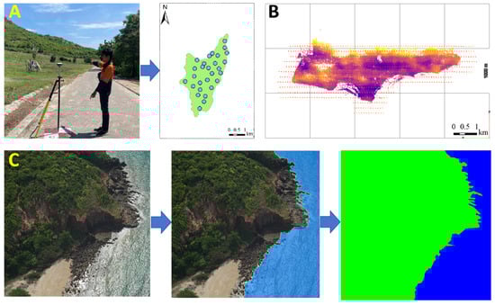
Figure 2.
Diagram of the UAV Survey and Data Processing Workflow. (A) Ground Control Points; (B) Unmanned Aerial Vehicle (UAV) Flight Path Planning; (C) Label Fabrication.
The data collection was completed on 17 May 2023. The planned flight route covered the entire shoreline of Koh Lan to obtain high-resolution imagery data for the entire island and coastal zone. From the original image set, 1000 images that clearly displayed shoreline features were manually selected and cropped into uniform blocks of 4000 × 4000 pixels to balance sea and land sample points and prevent biases and overfitting during the model training process.
This study employed the LabelMe image annotation tool to make precise annotations of the aerial images. During the annotation process, visual discrimination criteria were strictly followed, with land areas marked in green and sea areas marked in blue (as shown in Figure 2C). At the same time, full consideration was given to details such as topographic features, vegetation cover, and water body boundaries, which are crucial for constructing a high-quality training dataset and ensuring the model’s accuracy in image segmentation tasks. The annotated data in JSON format were converted into PNG image files through the PyCharm platform to ensure compatibility with different analysis tools.
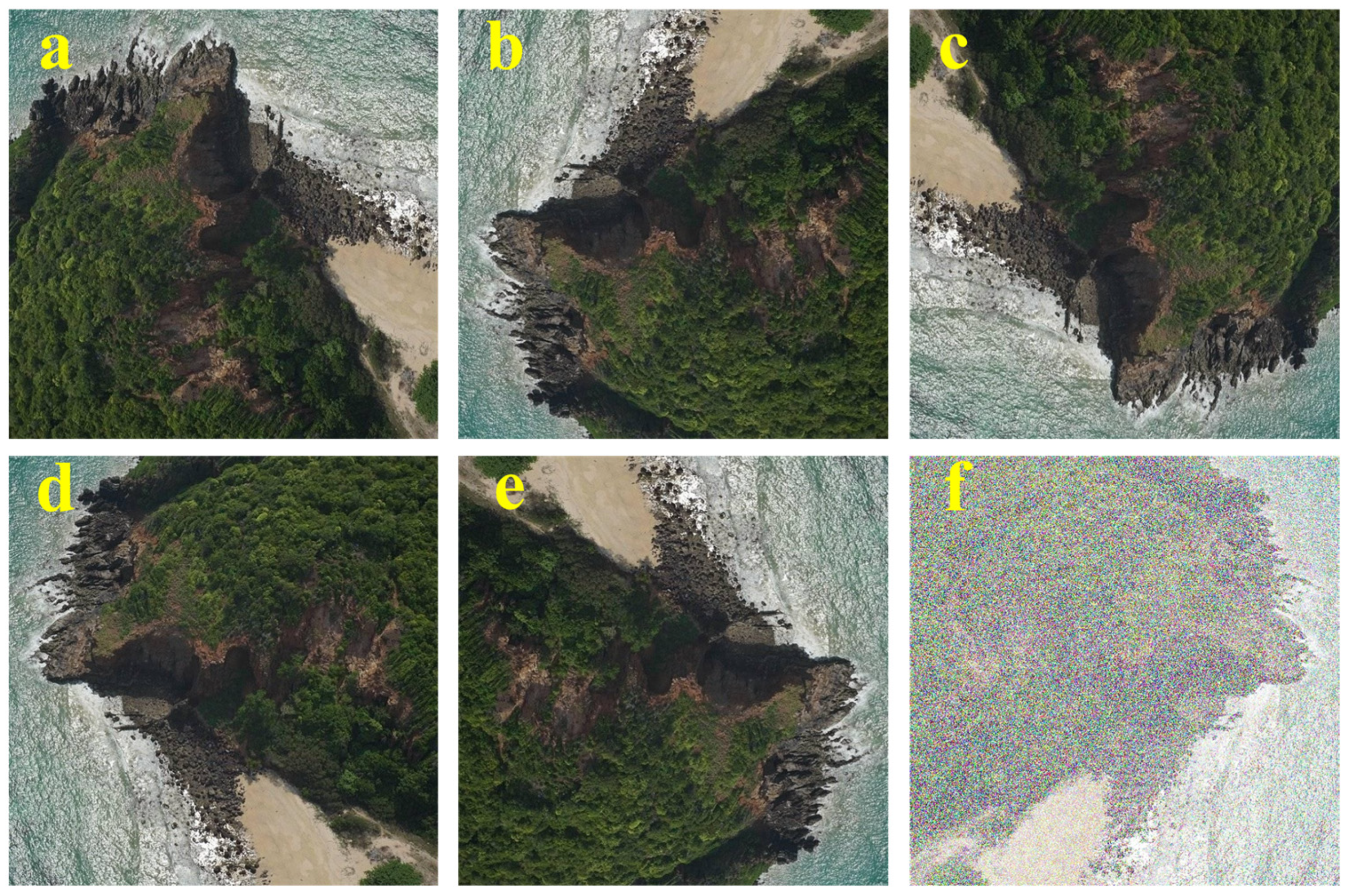
To effectively expand the scale of the training samples, this study employed data augmentation techniques on the dataset. The specific methods included random rotation of images (90°, 180°, 270°), horizontal and vertical flipping, and the introduction of Gaussian noise (Figure 3). After augmentation, a total of 7000 images were produced and divided according to a 9:1 ratio, creating a training set of 6300 images and a validation set of 700 images.

Figure 3.
Data augmentation example. (a) Rotation 90°; (b) Rotation 180°; (c) Rotation 270°; (d) Horizontal Flipping; (e) Vertical Flipping; (f) Adding Gaussian Noise.
2.1.3. Training Environment Setup
The experimental hardware environment for this study is detailed in Table 2, and all experiments were conducted strictly according to the configurations listed. The Adam optimization algorithm was used for model training, with an initial learning rate of 0.0001, a batch size of 8, and an initial epoch set to 200. To monitor the training process and save the best model state, model parameters were saved every 4 epochs for subsequent evaluation and selection of the optimal model.
Table 2.
Experimental setup parameters.
2.2. Construction of the Optimized DeepLabV3+ Model
This study constructed an optimized DeepLabV3+ model, the overall network structure of which is shown in Figure 4A. The main improvements made to the DeepLabV3+ model include: (1) the use of the MobileNetV2 network as the backbone for feature extraction, replacing the original backbone network. This improvement not only reduces the number of model parameters and computational complexity but also enhances the model’s ability to capture key visual features. (2) Innovatively introduced a Strip Pooling Layer in the ASPP (Atrous Spatial Pyramid Pooling) layer of the model, effectively expanding the receptive field of the network and enabling it to capture long-range dependencies within the image; (3) The model integrates the CBAM (Convolutional Block Attention Module) attention mechanism after low-dimensional feature extraction and before upsampling, allowing the model to adaptively focus on key areas of the image, thereby endowing the model with greater flexibility and adaptability during the feature extraction process.
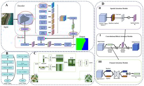
Figure 4.
Improvement of DeepLabV3+ schematic diagram. (A) Overall framework of the improved DeepLabV3+ model, Input: Original Shoreline Image, Output: Shoreline Label Image; (B) Inverted residual structure of MobileNetV2; (C) Schematic diagram of the strip pooling layer; (D) CBAM attention mechanism.
2.2.1. Backbone Extraction Network Replacement
In response to the complexity, large parameter size, and high computational cost of the Xception backbone network, this study introduces MobileNetV2, which is specifically designed for resource-constrained environments, to replace the original backbone network. This replacement aims to reduce computational load and enhance feature extraction capabilities. Its core advantage lies in the innovative inverted residual structure with a linear bottleneck (Figure 4B), which first increases the dimensionality through 1 × 1 convolutions to enhance feature representation, then reduces the dimensionality using depthwise separable convolutions, thereby maintaining sensitivity to key visual features while reducing the number of parameters and computational complexity. Finally, information fusion is achieved through residual connections with the original features.
2.2.2. Strip Pooling Layer
In shoreline extraction scenarios, due to the continuous and slender characteristics of shorelines, conventional global pooling struggles to accurately capture their features. To address the shortcomings of deep convolutional networks [48], multi-scale feature fusion [49], dilated convolutions, and pyramid network structures in capturing irregular or anisotropic contextual information, this study introduces a Strip Pooling layer into the Atrous Spatial Pyramid Pooling (ASPP) module of the original network architecture, as shown in Figure 4C. Strip Pooling utilizes long and narrow kernels (1 × N or N × 1) to expand the receptive field of the network, capturing long-range dependencies within the image more effectively.
The main process of Strip Pooling includes: (1) Input feature map: The input is a feature map with dimensions C × H × W (where C represents the number of channels, H represents the height of the feature map, and W represents the width of the feature map.); (2) Strip pooling: The feature map undergoes strip pooling in both the horizontal and vertical directions, with pooling kernels of 1 × N or N × 1, resulting in feature maps of dimensions H × 1 and 1 × W, where the pooling result is the average value of pixels within the strip region. (3) Feature Enhancement: After the strip pooling process, 1D convolution is applied to the feature maps to restore the number of channels to that of the input feature map, which is C × H × W. (4) Feature fusion and activation: The features are fused through 1 × 1 convolution and then subjected to a Sigmoid activation function for nonlinear transformation. Finally, they are multiplied pixel by pixel with the input feature map to obtain the final output.
2.2.3. CBAM Attention Mechanism
The attention mechanism has become one of the key technologies for enhancing the performance of deep learning models [50].CBAM (Convolutional Block Attention Module) is a lightweight module that combines channel attention and spatial attention, as shown in Figure 4D, effectively enhancing the model’s recognition of key image features. Its design not only saves computational effort but also effectively improves the model’s attention effects.
Channel Attention Module (CAM), as shown in Figure 4D(III): It captures the statistical information between channels through global average pooling and max pooling operations, then uses a multi-layer perceptron (MLP) to learn the dependencies among channels, generating channel weights for weighted processing of each channel (Equation (1) [51]).
where F is the input feature map, AvgPool(F) and MaxPool(F) respectively obtain the global information of each channel through global average pooling and global max pooling, MLP is the multi-layer perceptron, σ is the Sigmoid activation function, and Mc(F) is the channel attention weight map.
Spatial Attention Module (SAM), as shown in Figure 4D(II): It extracts spatial information through average pooling and max pooling, concatenates them, and then processes through a 7 × 7 convolution to generate spatial weights, highlighting key areas in the image (Equation (2) [51]).
where F is the input feature map, AvgPool(F) and MaxPool(F) capture spatial features through average pooling and max pooling respectively, f 7×7 denotes the 7 × 7 convolution, σ is the Sigmoid activation function, and Ms(F) is the spatial attention weight map.
2.2.4. Loss Function and Evaluation Metrics
To enhance numerical stability and simplify the model training process, while also optimizing the performance of binary classification tasks, this study employed BCEWithLogitsLoss as the loss function. This function is a variant of the binary cross-entropy loss (BCELoss), combining the Sigmoid activation function and BCELoss, allowing the model to directly learn unnormalized prediction values (logits). This approach prevents the vanishing or exploding gradient problem caused by the output range of the Sigmoid function (between 0 and 1). The definition of the loss function is given in Equation (3) [52]:
where y represents the true labels, z represents the raw output (logits) of the model, and σ represents the Sigmoid function.
Additionally, this study employed four evaluation metrics to assess the model’s performance, which are Pixel Accuracy (PA), Recall, F1 Score, and Intersection over Union (IoU). The specific calculations are given in Equation (4) [53]
where TP represents true positives (the model predicts positive and it is actually positive), FP represents false positives (the model predicts positive but it is actually negative), FN represents false negatives (the model predicts negative but it is actually positive), and TN represents true negatives (the model predicts negative and it is actually negative).
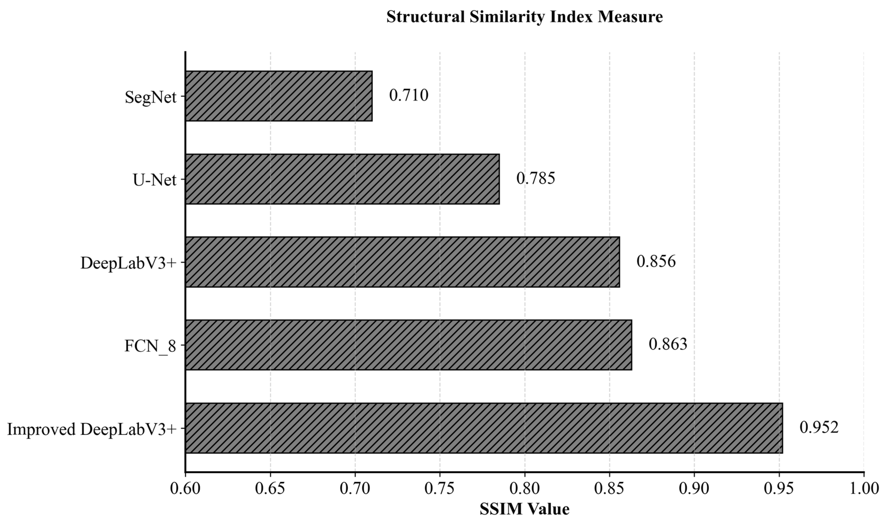
To further evaluate the spatial consistency and perceptual quality of predictions, we additionally adopted the Structural Similarity Index Measure (SSIM) [54], which quantifies the similarity in luminance, contrast, and structural patterns between predictions and references. It complements pixel-level metrics by emphasizing spatial coherence in complex coastal feature extraction tasks. The SSIM is calculated as:
where μx and μy represent the mean intensity of the predicted image x and the ground truth y, respectively; σx and σy represent the standard deviation of x and y; σxy represents the covariance between x and y; and C1 and C2 are stabilization constants to avoid division by zero.
3. Results
3.1. Training Results of Different Attention Mechanisms
To comprehensively evaluate the performance improvement of attention mechanisms on the improved DeepLabV3+ model, this study conducted a systematic comparison, analyzing three advanced attention mechanisms: Channel Attention (CA) [55], Squeeze-and-Excitation Networks (SE-Net) [56], and Convolutional Block Attention Module (CBAM). These mechanisms are strategically embedded in two critical stages of the model: shallow feature extraction and deep feature upsampling. The shallow layer is responsible for capturing the basic visual patterns of the image, while the deep layer integrates and refines these features.
The results shown in Table 3 reveal the impact of integrating three different attention mechanism modules on the performance of the improved DeepLabV3+ network. Among them, the CBAM attention mechanism showed particularly outstanding performance. Compared to the original network, the introduction of the CBAM attention mechanism increased the precision (PA) by 3.1%, and the Intersection over Union (IoU) was improved by 8.2%. Following the CBAM attention mechanism is the SE-Net attention mechanism, which increased PA and IoU by 2.9% and 7.7%, respectively. Although the CA attention mechanism showed a smaller improvement, it still achieved a 1.9% increase in PA and a 6.6% increase in IoU.
Table 3.
Results of attention mechanism selection.
3.2. Segmentation Accuracy Evaluation
To verify the effectiveness of the improved DeepLabV3+ model in shoreline extraction tasks, the study conducted a comprehensive comparison with FCN8, SegNet, U-Net, and the original DeepLabV3+ model. All models were evaluated under the same training parameters and conditions to ensure the fairness of the comparison and the reliability of the results.
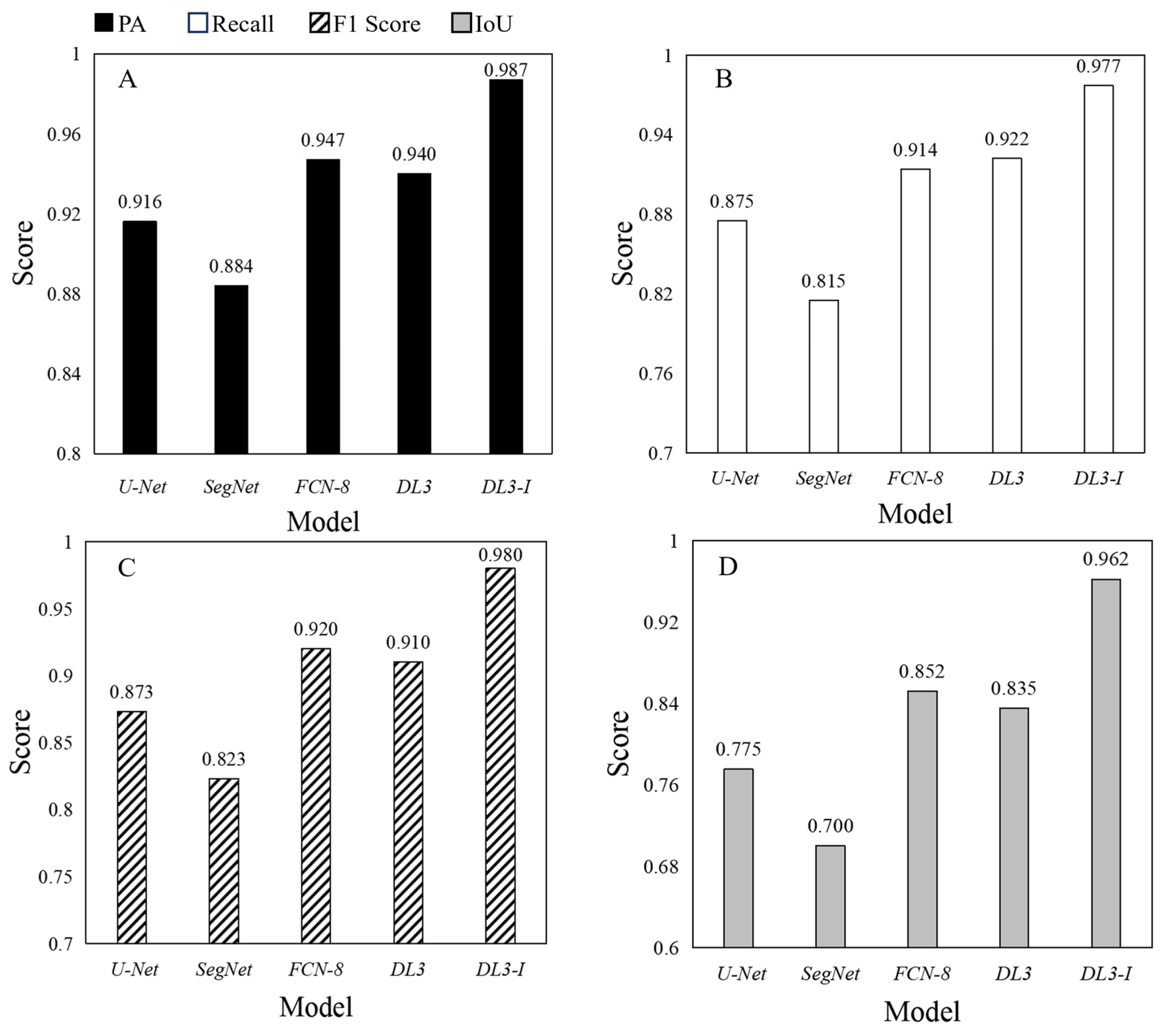
Figure 5 comprehensively presents the performance of various models on segmentation accuracy metrics, including Pixel Accuracy (PA), Recall, F1 Score, and Intersection over Union (IoU). Among them, the improved DeepLabV3+ model showed excellent performance in all evaluation metrics, with PA reaching 98.7%, Recall at 97.7%, F1 Score at 98.0%, and IoU at 96.2%. Compared to the original DeepLabV3+ model, the improvements in each metric were 4.7%, 5.5%, 7%, and 12.7%, respectively. Compared to FCN8, SegNet, and U-Net, the improved DeepLabV3+ model achieved enhancements of 4%, 10.3%, and 7.1%, 6.3%, 16.2%, and 10.2%, 6.0%, 15.7%, and 10.7%, as well as 11.0%, 26.2%, and 18.7% in PA, Recall, F1 Score, and IoU, respectively.

Figure 5.
Comparison of segmentation accuracy results for five models. where DL3 denotes the DeepLabV3+ model and DL3-I signifies the DeepLabV3+_Improved model. (A) illustrates the comparison of pixel accuracy (PA) metrics, (B) depicts the recall metrics, (C) presents the F1-score metrics, and (D) shows the intersection over union (IoU) metrics.
3.3. Model Efficiency Evaluation
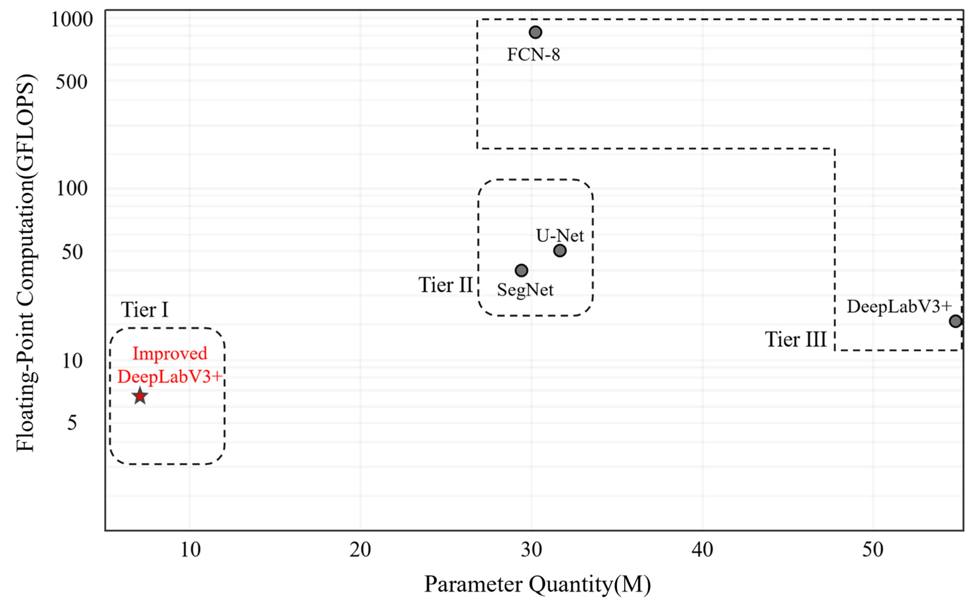
In practical applications, model efficiency is a crucial consideration factor, directly affecting the deployability and practicality of the model. This study compared the improved DeepLabV3+ model with other existing models in terms of parameter quantity and floating-point operations (GFLOPS) through Figure 6. The improved DeepLabV3+ model showed the lowest resource consumption among all models tested, with a parameter quantity of 6.61 M and a floating-point operation count of 6.7 GFLOPS.
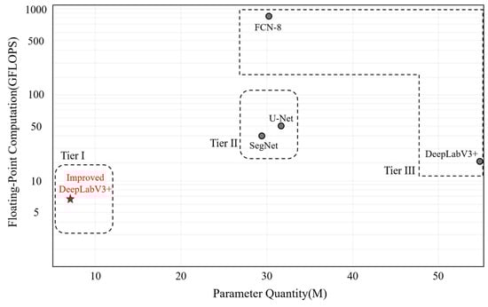
Figure 6.
Schematic diagram of model performance indicators. The points in the lower left represent models with fewer parameters and less floating-point computation, where Tier I represents models in the first echelon, Tier II represents models in the second echelon, and Tier III represents models in the third echelon.
The specific comparison results are shown in Figure 6. Compared to the FCN8 model, the improved DeepLabV3+ model achieved about an 80% reduction in parameter quantity and a 92% reduction in floating-point operations. Compared to the SegNet model, the reductions in parameter quantity and floating-point operations were 80% and about 86%, respectively. Compared to the U-Net model, the improved model reduced the parameter quantity by 80% and the floating-point operations by about 88%. Compared to the original DeepLabV3+ model, the improved model also reduced the parameter quantity by about 88% and the floating-point operations by about 67%. These reductions are primarily attributed to replacing the Xception backbone network with MobileNetV2, which employs an inverted residual structure with a linear bottleneck. This structure first expands the dimensions via 1 × 1 convolutions to enhance feature representation, then reduces the dimensions using depthwise separable convolutions, thereby maintaining sensitivity to key visual features while decreasing the number of parameters and computational complexity. Additionally, residual connections facilitate information fusion with the original features, further optimizing the model’s efficiency and performance.
4. Discussion
4.1. Comparison of Attention Mechanism Training Effects
Yin et al. [57] have shown that by introducing the CBAM attention mechanism to the PSPNet (Pyramid Scene Parsing Network) model, the network’s ability to recognize key image features was enhanced, leading to more accurate water-land segmentation. This study also shows the same pattern, as shown in Table 3. This finding emphasizes the importance of considering both channel and spatial information in the process of capturing key image features.
Furthermore, integrating the attention mechanism before the deep feature upsampling stage, compared to only after the shallow feature extraction stage, can achieve more performance improvements. The reason is that deep features are rich in semantic information, which often includes important semantic content of the image, such as the shape and texture of objects. Additionally, the deep feature upsampling stage is a critical period for integrating high-level semantic information with low-level pixel-level detail information. Applying the attention mechanism at this stage helps the model more accurately identify which low-level features are critical, thereby selectively enhancing these features during the upsampling process while suppressing noise and unimportant information.
4.2. Comprehensive Analysis of Improved Algorithm Performance
In this section, we conducted a comprehensive evaluation of the performance impact of the introduced CBAM attention mechanism module, MobileNetV2 module, and Strip Pooling layer module on the improved DeepLabV3+ model. For specific data, see Table 4.
Table 4.
Performance Evaluation of the Improved DeepLabV3+ Model.
In terms of the accuracy of shoreline extraction, the improved DeepLabV3+ model demonstrated exceptional performance. Particularly, the introduction of the Strip Pooling layer, an innovative design specifically targeting the feature capture of linear features such as shorelines, enhanced the model’s F1-Score and IoU metrics by 4.4% and 7.5%, greatly increasing the precision of feature extraction. Furthermore, the integrated Convolutional Block Attention Module (CBAM) further enhanced the model’s expressive power for key features, with the F1-Score and IoU metrics improving by an additional 2.8% and 4.8%, respectively. CBAM, through its fine-grained channel attention and spatial attention mechanisms, endowed the model with an adaptive focusing capability on key features, enhancing the model’s representation and decision-making accuracy in shoreline extraction tasks.
In terms of model efficiency, the improved DeepLabV3+ also performed exceptionally well. By using MobileNetV2 as the backbone network, the GFLOPS metric was reduced by 48.89, and the parameter count was lowered by 14.19 M, achieving a reduction in both parameter volume and floating-point computations. Compared to traditional models and other comparative models, it is more economical in terms of resource consumption.
Yang et al. 2020 [58] created a benchmark dataset for land-sea boundary segmentation based on Landsat-8 imagery data and compared the performance of various advanced models on the land-sea boundary segmentation task. The results showed that DeepLabV3+ and FC-DenseNet achieved the best performance, and considering the training time efficiency, DeepLabV3+ performed better in land-sea segmentation. These findings are highly consistent with the optimal results obtained in this study after improving the DeepLabV3+ model in terms of performance and efficiency. Aghdami-Nia et al. [59] successfully improved the accuracy of shoreline extraction by modifying the standard U-Net (SUN) model. The study’s test results on two datasets showed that, compared to the current leading models FC-DenseNet and DeepLabV3+, the improved SUN model had higher segmentation accuracy. However, in this study, the improved DeepLabV3+ model outperformed the U-Net model, achieving an IoU of 96.2% compared to the U-Net model’s 77.5%. This enhancement is mainly due to two factors: First, the combination of the CBAM attention mechanism and strip pooling layer improved the model’s ability to capture detailed shoreline boundaries and reduce background noise, which is crucial for optimizing IoU. Second, the high–resolution drone dataset (1.5 cm/pixel) used in this study provided richer spatial and textural details than the satellite data (10–30 m/pixel) used in Aghdami-Nia et al.’s study, allowing for more precise differentiation of subtle shoreline features such as tidal flats and artificial structures. These improvements highlight the significance of both algorithmic refinement and high–quality data in advancing shoreline extraction tasks.
In summary, the improved DeepLabV3+ model not only achieved improvements in segmentation accuracy but also made notable progress in model efficiency, fully demonstrating its broad application prospects and practical value in complex visual tasks such as high-precision shoreline extraction. These improvements enable the model to provide more accurate shoreline extraction results and to operate efficiently in resource-constrained environments, providing strong technical support for shoreline monitoring and management.
4.3. Performance Superiority of Improved Algorithm in Different Coastline Extraction Conditions
To explore the performance of the improved DeepLabV3+ model in different shoreline extraction scenarios, this study used FCN8, SegNet, U-Net, and the original DeepLabV3+ models as comparative models to extract shorelines from the verification set. The island shoreline images in the verification set were classified into three types: natural shorelines, artificial shorelines, and composite shorelines. Representative areas were selected from each type for in-depth analysis and comparison.
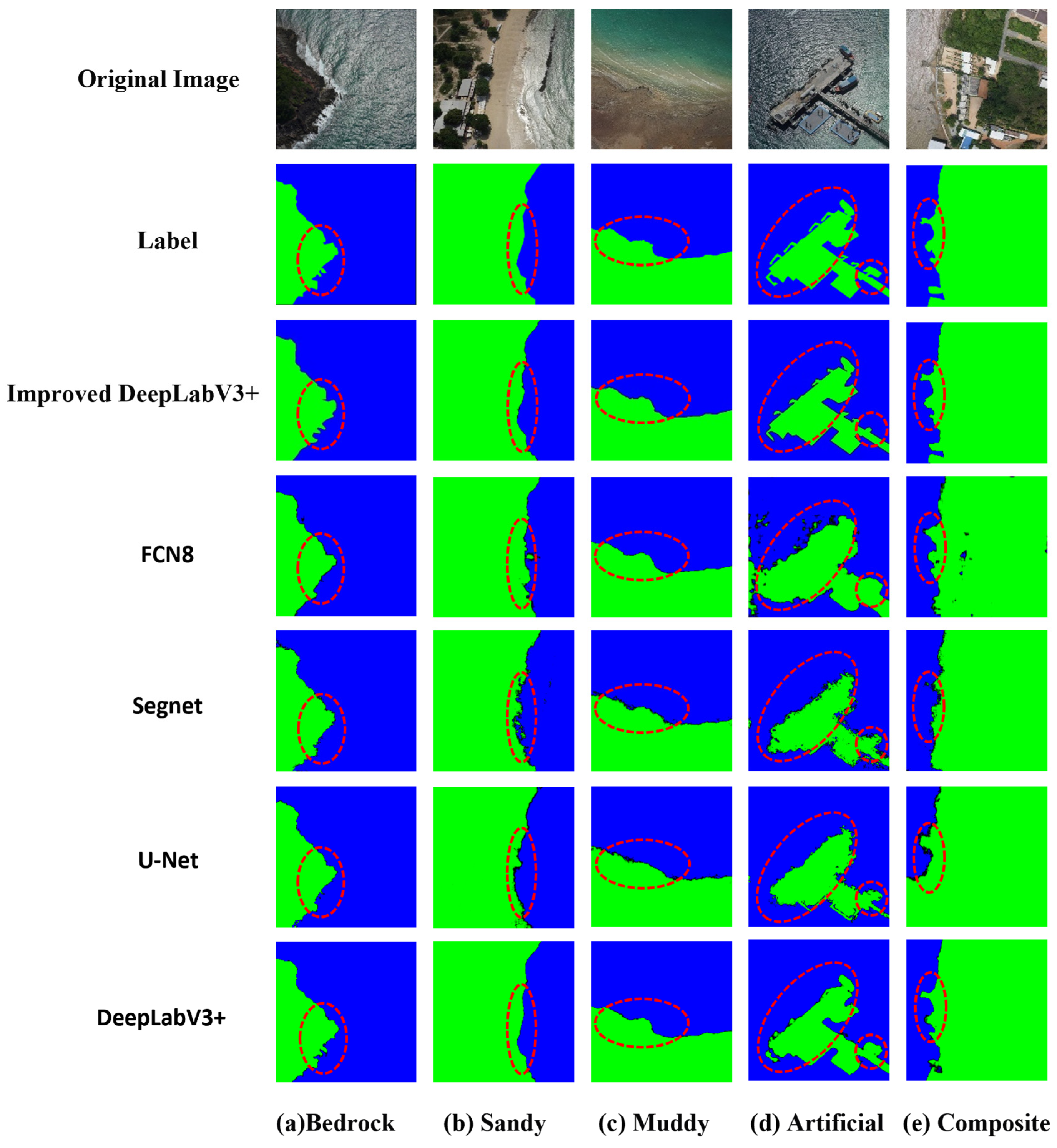
Figure 7 indicates that while all five algorithms can identify the general location of the shoreline to some extent, the improved DeepLabV3+ model performs exceptionally well in different shoreline extraction tasks, especially in terms of detail and boundary accuracy, which is better than the other models. Figure 8 shows that the improved DeepLabV3+ model maintains the best spatial consistency in shoreline segmentation, with SSIM values increased by 8.9% compared to FCN8, 11.2% compared to the original DeepLabV3+, and 21.3% and 34.1% compared to U-Net and SegNet, respectively. Specifically:

Figure 7.
Visual Comparison of Five Typical Shoreline Segmentations.

Figure 8.
SSIM Performance of Five Coastal Segmentation Algorithms.
In the extraction of bedrock natural shorelines, compared to FCN8, SegNet, U-Net, and the original DeepLabV3+ models, the improved DeepLabV3+ was more accurate in segmenting small bedrock areas, effectively reducing misclassification and omissions, and was highly consistent with the true labels. In the extraction of sandy shorelines, the FCN8, U-Net, and SegNet models resulted in fragmented and blurry outcomes due to the loss of boundary information. Notably, the U-Net model misidentified the white crown formed by seawater hitting the beach as land, leading to misclassification. In contrast, the improved DeepLabV3+ was essentially consistent with the labels. In the extraction of muddy shorelines, the spectral features of the muddy flats were similar to those of the land, causing the SegNet and U-Net models to have false positives and omissions due to shadowing phenomena. However, the improved model achieved the best results with the fewest false positives and omissions.
For the extraction of artificial shorelines, the FCN8 model mistakenly classified some seawater as land due to the loss of boundaries. The SegNet and U-Net models, in the early stages of feature extraction, were unable to accurately recognize the detailed features of artificial shorelines due to their small receptive fields, leading to fragmentation and blurriness. The DeepLabV3+ model, while able to clearly segment the main body of the dock, showed fragmentation in identifying small protruding structures of the dock. In contrast, the improved DeepLabV3+ model performed the best in extracting the main body of the dock, accurately identifying small protruding structures without fragmentation, and had the fewest omissions and misclassifications.
In the extraction of composite shorelines, the FCN8 model mistakenly identified blue houses as seawater, resulting in a poor visual effect. The U-Net model, due to its small receptive field, lost some boundary information and mistakenly classified parts of the seawater as land. The SegNet and original DeepLabV3+ models showed blurriness when dealing with complex shoreline structures due to insufficient extraction capabilities. The improved model, however, demonstrated the most complete segmentation effect, avoiding the common issues of blurriness, fragmentation, and loss of boundary information seen in other models.
In shoreline extraction research, this study found that the complex characteristics of different shoreline types pose challenges to deep learning models. Natural shorelines are relatively easy to identify due to their simple textures and clear spectral contrasts, while artificial and composite shorelines are difficult to distinguish because of their complex textures and spectral features. The improved DeepLabV3+ model, with its advanced network structure, performs well in these complex scenarios, effectively capturing subtle texture changes and surpassing the extraction accuracy of other models.
4.4. Future Outlook and Directions for Improvement
Although the improved DeepLabV3+ model has shown excellent performance in shoreline extraction tasks, it still faces challenges under specific conditions. Particularly in extreme weather [60] or under strong lighting changes, excessive blurring or damage to images can lead to a decline in model performance, thereby affecting the accuracy of shoreline extraction. Moreover, for shorelines with similar spectral features, such as muddy flats [61], the model still needs to improve in recognizing subtle texture and pattern changes. To address these challenges, future research directions should include the development of more refined feature extraction strategies and the exploration of new model optimization methods, such as introducing more advanced network architectures to enhance the recognition of detailed features. At the same time, improving the model’s robustness through data augmentation techniques is expected to further optimize the model, enabling it to adapt to more complex and variable real-world application environments.
It is worth noting that this study primarily focuses on the high-precision extraction of instantaneous shorelines and does not cover the prediction of dynamic shoreline changes. However, it lays the groundwork for future research on dynamic shoreline change processes. Therefore, future research will focus on the study of dynamic shorelines to further advance our understanding and predictive capabilities regarding shoreline evolution.
5. Conclusions
In this study, we conducted an in-depth optimization of the DeepLabV3+ model by integrating MobileNetV2, CBAM attention mechanism, and Strip Pooling Layer, developing an efficient method for remote sensing shoreline extraction of islands. Here is a detailed summary of the research findings:
(1) The improved DeepLabV3+ model showed a significant leading advantage in performance metrics compared to FCN8, SegNet, U-Net, and the original DeepLabV3+ model when evaluated on the Koh Lan Island drone dataset (1.5 cm/pixel). Specifically, PA, Recall, F1-Score, and IoU achieved improvements of 4.0%, 10.3%, 7.1%, 4.7%; 6.2%, 16.2%, 10.2%, 5.5%; 16.0%, 15.7%, 10.7%, 7.0%, and 11.0%, 26.2%, 18.7%, 12.7% respectively. In terms of model efficiency, the improved DeepLabV3+ model has a parameter count of 6.61 M and a floating-point computation of 6.7 GFLOP, which are reduced compared to the aforementioned models, achieving dual optimization of accuracy and efficiency.
(2) In this study, the CBAM attention mechanism was introduced in the shallow feature extraction and deep feature upsampling stages of the model. Compared to the SE-Net and CA attention mechanisms, the CBAM attention mechanism significantly improved the accuracy of shoreline extraction, with PA metrics increasing by 0.2% and 1.2%, and IoU metrics increasing by 0.5% and 1.6%, respectively. Additionally, the experimental results showed that integrating the attention mechanism before the deep feature upsampling stage, compared to integrating it only after shallow feature extraction, resulted in a 0.4% increase in PA and a 0.8% increase in IoU, achieving more significant performance improvements.
(3) The improved DeepLabV3+ model demonstrated outstanding performance in various shoreline extraction tasks, with high visual and structural consistency between predictions and ground truth labels. The model was able to effectively distinguish between shadows and water bodies, reducing the occurrence of missed and false detections. It decreased the probability of common issues such as blurriness, fragmentation, and loss of boundary information found in other models, thereby lowering the risk of misclassification and presenting the most complete shoreline segmentation results.
Additionally, the improved DeepLabV3+ model not only achieves technical innovation but also has broad application value. It can be used to analyze the prevention and emergency response to disasters such as coastal erosion, sedimentation, and storm surges, as well as environmental monitoring and assessment tasks such as sea-level rise. By providing accurate shoreline data, the model can offer foundational data support for the rational planning and management of coastal zones, contributing to the sustainable development and utilization of coastal resources and preventing environmental damage caused by overdevelopment.
Author Contributions
Conceptualization, Z.G. and Z.Z.; methodology, Z.G. and J.S.; investigation, S.P. and C.J.; resources, S.P. and C.J.; data curation, J.M., H.N. and Y.Q.; writing—original draft preparation, J.S.; writing—review and editing, Z.G.; supervision, Z.Z.; funding acquisition, Z.G. All authors have read and agreed to the published version of the manuscript.
Funding
This research was supported by the National Foundation of Natural Sciences of China (Grant Nos. 42171292, 42376228), the Special Fund for Asian Regional Cooperation from the China Ministry of Foreign Affairs (Grant No. WJ1324008), and the China Oceanic Development Foundation (Grant No. B222023017).
Data Availability Statement
Data will be made available on request.
Acknowledgments
Thank you to the Thailand Department of Marine and Coastal Resources (DMCR) and the Intergovernmental Oceanographic Commission Sub-Commission for the Western Pacific (IOC-WESTPAC) for their strong support in conducting this research.
Conflicts of Interest
The authors declare no conflicts of interest.
References
- Li, J.; Chu, S.; Hu, Q.; Cong, Y.; Cheng, J.; Chen, H.; Cheng, L.; Zhang, G.; Xing, S. Land-sea classification based on the fast feature detection model for ICESat-2 ATL03 datasets. Int. J. Appl. Earth Obs. Geoinf. 2024, 130, 103916. [Google Scholar] [CrossRef]
- Mao, Y.; Harris, D.L.; Xie, Z.; Phinn, S.; Sensing, R. Efficient measurement of large-scale decadal shoreline change with increased accuracy in tide-dominated coastal environments with Google Earth Engine. ISPRS J. Photogramm. Remote Sens. 2021, 181, 385–399. [Google Scholar] [CrossRef]
- Liu, L.; Xu, W.; Yue, Q.; Teng, X.; Hu, H. Problems and countermeasures of coastline protection and utilization in China. Ocean Coast Manage. 2018, 153, 124–130. [Google Scholar] [CrossRef]
- Arkema, K.K.; Verutes, G.M.; Wood, S.A.; Clarke-Samuels, C.; Rosado, S.; Canto, M.; Rosenthal, A.; Ruckelshaus, M.; Guannel, G.; Toft, J. Embedding ecosystem services in coastal planning leads to better outcomes for people and nature. Proc. Natl. Acad. Sci. USA 2015, 112, 7390–7395. [Google Scholar] [CrossRef]
- Martínez, C.; Contreras-López, M.; Winckler, P.; Hidalgo, H.; Godoy, E.; Agredano, R. Coastal erosion in central Chile: A new hazard? Ocean Coast Manage. 2018, 156, 141–155. [Google Scholar] [CrossRef]
- Xu, N.; Gong, P. Significant coastline changes in China during 1991–2015 tracked by Landsat data. Sci. Bull. 2018, 63, 883–886. [Google Scholar] [CrossRef]
- Cáceres, F.; Wadsworth, F.B.; Scheu, B.; Colombier, M.; Madonna, C.; Cimarelli, C.; Hess, K.-U.; Kaliwoda, M.; Ruthensteiner, B.; Dingwell, D.B. Can nanolites enhance eruption explosivity? Geology 2020, 48, 997–1001. [Google Scholar] [CrossRef]
- Qiao, G.; Mi, H.; Wang, W.; Tong, X.; Li, Z.; Li, T.; Liu, S.; Hong, Y. 55-year (1960–2015) spatiotemporal shoreline change analysis using historical DISP and Landsat time series data in Shanghai. Int. J. Appl. Earth Obs. Geoinf. 2018, 68, 238–251. [Google Scholar] [CrossRef]
- Turner, I.L.; Harley, M.D.; Drummond, C.D. UAVs for coastal surveying. Coast. Eng. 2016, 114, 19–24. [Google Scholar] [CrossRef]
- Himmelstoss, E.A.; Henderson, R.E.; Farris, A.S.; Kratzmann, M.G.; Ergul, A.; McAndrews, J.; Cibaj, R.; Zichichi, J.L.; Thieler, E.R. Digital Shoreline Analysis System Version 6.0; US Geological Survey: Reston, VA, USA, 2024.
- Troy, C.D.; Cheng, Y.-T.; Lin, Y.-C.; Habib, A. Rapid lake Michigan shoreline changes revealed by UAV LiDAR surveys. Coast. Eng. 2021, 170, 104008. [Google Scholar] [CrossRef]
- Mentaschi, L.; Vousdoukas, M.I.; Pekel, J.-F.; Voukouvalas, E.; Feyen, L. Global long-term observations of coastal erosion and accretion. Sci. Rep. 2018, 8, 12876. [Google Scholar] [CrossRef]
- Ataol, M.; Kale, M.M. Shoreline changes in the river mouths of the Ceyhan Delta. Arab. J. Geosci. 2022, 15, 201. [Google Scholar] [CrossRef]
- Medhioub, E.; Hentati, I. A Shoreline Change Analysis Using Satellite Images Survey and DSAS Technique: A Case Study of Monastir-Chebba Coast, Tunisia; Springer: Cham, Switzerland, 2024; pp. 753–757. [Google Scholar]
- Hossain, M.S.; Yasir, M.; Wang, P.; Ullah, S.; Jahan, M.; Hui, S.; Zhao, Z. Automatic shoreline extraction and change detection: A study on the southeast coast of Bangladesh. Mar. Geol. 2021, 441, 106628. [Google Scholar] [CrossRef]
- Zhang, S.; Wu, L.; Arnqvist, J.; Hallgren, C.; Rutgersson, A. Mapping coastal upwelling in the Baltic Sea from 2002 to 2020 using remote sensing data. Int. J. Appl. Earth Obs. Geoinf. 2022, 114, 103061. [Google Scholar] [CrossRef]
- Shamsuzzoha, M.; Ahamed, T. Shoreline Change Assessment in the Coastal Region of Bangladesh Delta Using Tasseled Cap Transformation from Satellite Remote Sensing Dataset. Remote Sens. 2023, 15, 295. [Google Scholar] [CrossRef]
- Dai, C.; Howat, I.M.; Larour, E.; Husby, E. Coastline extraction from repeat high resolution satellite imagery. Remote Sens. Environ. 2019, 229, 260–270. [Google Scholar] [CrossRef]
- Paravolidakis, V.; Ragia, L.; Moirogiorgou, K.; Zervakis, M.E. Automatic Coastline Extraction Using Edge Detection and Optimization Procedures. Geosciences 2018, 8, 407. [Google Scholar] [CrossRef]
- Zhang, Z.; Lu, W.; Cao, J.; Xie, G. MKANet: An efficient network with Sobel boundary loss for land-cover classification of satellite remote sensing imagery. Remote Sens. 2022, 14, 4514. [Google Scholar] [CrossRef]
- Hu, X.; Wang, Y. Monitoring coastline variations in the Pearl River Estuary from 1978 to 2018 by integrating Canny edge detection and Otsu methods using long time series Landsat dataset. Catena 2022, 209, 105840. [Google Scholar] [CrossRef]
- Teng, J.; Xia, S.; Liu, Y.; Yu, X.; Duan, H.; Xiao, H.; Zhao, C. Assessing habitat suitability for wintering geese by using Normalized Difference Water Index (NDWI) in a large floodplain wetland, China. Ecol. Indic. 2021, 122, 107260. [Google Scholar] [CrossRef]
- Rashid, M.B. Monitoring of drainage system and waterlogging area in the human-induced Ganges-Brahmaputra tidal delta plain of Bangladesh using MNDWI index. Heliyon 2023, 9, e17412. [Google Scholar] [CrossRef]
- Cao, W.; Zhou, Y.; Li, R.; Li, X. Mapping changes in coastlines and tidal flats in developing islands using the full time series of Landsat images. Remote Sens. Environ. 2020, 239, 111665. [Google Scholar] [CrossRef]
- Wang, X.; Xiao, X.; Zou, Z.; Chen, B.; Ma, J.; Dong, J.; Doughty, R.B.; Zhong, Q.; Qin, Y.; Dai, S. Tracking annual changes of coastal tidal flats in China during 1986–2016 through analyses of Landsat images with Google Earth Engine. Remote Sens. Environ. 2020, 238, 110987. [Google Scholar] [CrossRef] [PubMed]
- Seale, C.; Redfern, T.; Chatfield, P.; Luo, C.; Dempsey, K. Coastline detection in satellite imagery: A deep learning approach on new benchmark data. Remote Sens. Environ. 2022, 278, 113044. [Google Scholar] [CrossRef]
- Wu, Y.; Liu, Z. Research progress on methods of automatic coastline extraction based on remote sensing images. Natl. Remote Sens. Bulletin. 2019, 23, 582–602. [Google Scholar] [CrossRef]
- Bi, Q.; Zhang, H.; Qin, K. Multi-scale stacking attention pooling for remote sensing scene classification. Neurocomputing 2021, 436, 147–161. [Google Scholar] [CrossRef]
- Zou, Q.; Ni, L.; Zhang, T.; Wang, Q. Deep learning based feature selection for remote sensing scene classification. IEEE Geosci. Remote Sens. Lett. 2015, 12, 2321–2325. [Google Scholar] [CrossRef]
- Wang, X.; Zhao, Q.; Jiang, P.; Zheng, Y.; Yuan, L.; Yuan, P. LDS-YOLO: A lightweight small object detection method for dead trees from shelter forest. Comput. Electron. Agric. 2022, 198, 107035. [Google Scholar] [CrossRef]
- Bayraktar, E.; Basarkan, M.E.; Celebi, N. A low-cost UAV framework towards ornamental plant detection and counting in the wild. ISPRS J. Photogramm. Remote Sens. 2020, 167, 1–11. [Google Scholar] [CrossRef]
- Diakogiannis, F.I.; Waldner, F.o.; Caccetta, P.; Wu, C. ResUNet-a: A deep learning framework for semantic segmentation of remotely sensed data. ISPRS J. Photogramm. Remote Sens. 2020, 162, 94–114. [Google Scholar] [CrossRef]
- Dang, K.B.; Vu, K.C.; Nguyen, H.; Nguyen, D.A.; Nguyen, T.D.L.; Pham, T.P.N.; Giang, T.L.; Nguyen, H.D.; Do, T.H. Application of deep learning models to detect coastlines and shorelines. J. Environ. Manag. 2022, 320, 115732. [Google Scholar] [CrossRef]
- Scala, P.; Manno, G.; Ciraolo, G. Semantic segmentation of coastal aerial/satellite images using deep learning techniques: An application to coastline detection. Comput. Geosci. 2024, 192, 105704. [Google Scholar] [CrossRef]
- Feng, J.; Wang, S.; Gu, Z. A Novel Sea-Land Segmentation Network for Enhanced Coastline Extraction using Satellite Remote Sensing Images. Adv. Space Res. 2024, 74, 5. [Google Scholar] [CrossRef]
- Aryal, B.; Escarzaga, S.M.; Vargas Zesati, S.A.; Velez-Reyes, M.; Fuentes, O.; Tweedie, C. Semi-Automated Semantic Segmentation of Arctic Shorelines Using Very High-Resolution Airborne Imagery, Spectral Indices and Weakly Supervised Machine Learning Approaches. Remote Sens. 2021, 13, 4572. [Google Scholar] [CrossRef]
- Xu, Y.; Ma, B.; Yu, G.; Zhang, R.; Tan, H.; Dong, F.; Bian, H. Accurate cotton verticillium wilt segmentation in field background based on the two-stage lightweight DeepLabV3+ model. Comput. Electron. Agric. 2025, 229, 109814. [Google Scholar] [CrossRef]
- Du, S.; Du, S.; Liu, B.; Zhang, X. Incorporating DeepLabv3+ and object-based image analysis for semantic segmentation of very high resolution remote sensing images. Int. J. Digit. Earth. 2021, 14, 357–378. [Google Scholar] [CrossRef]
- Pires de Lima, R.; Marfurt, K. Convolutional neural network for remote-sensing scene classification: Transfer learning analysis. Remote Sens. 2019, 12, 86. [Google Scholar] [CrossRef]
- Karadal, C.H.; Kaya, M.C.; Tuncer, T.; Dogan, S.; Acharya, U.R. Automated classification of remote sensing images using multileveled MobileNetV2 and DWT techniques. Expert Syst. Appl. 2021, 185, 115659. [Google Scholar] [CrossRef]
- Qu, Y.; Xia, M.; Zhang, Y. Strip pooling channel spatial attention network for the segmentation of cloud and cloud shadow. Comput. Geosci. 2021, 157, 104940. [Google Scholar] [CrossRef]
- He, C.; Liu, Y.; Wang, D.; Liu, S.; Yu, L.; Ren, Y. Automatic extraction of bare soil land from high-resolution remote sensing images based on semantic segmentation with deep learning. Remote Sens. 2023, 15, 1646. [Google Scholar] [CrossRef]
- Yang, X.; Li, S.; Chen, Z.; Chanussot, J.; Jia, X.; Zhang, B.; Li, B.; Chen, P. An attention-fused network for semantic segmentation of very-high-resolution remote sensing imagery. ISPRS J. Photogramm. Remote Sens. 2021, 177, 238–262. [Google Scholar] [CrossRef]
- Zheng, X.; Huan, L.; Xia, G.-S.; Gong, J. Parsing very high resolution urban scene images by learning deep ConvNets with edge-aware loss. ISPRS J. Photogramm. Remote Sens. 2020, 170, 15–28. [Google Scholar] [CrossRef]
- Su, Z.; Li, W.; Ma, Z.; Gao, R. An improved U-Net method for the semantic segmentation of remote sensing images. Appl. Intell. 2022, 52, 3276–3288. [Google Scholar] [CrossRef]
- Gonçalves, R.M.; Saleem, A.; Queiroz, H.A.A.; Awange, J.L. A fuzzy model integrating shoreline changes, NDVI and settlement influences for coastal zone human impact classification. Appl. Geogr. 2019, 113, 102093. [Google Scholar] [CrossRef]
- Ghosh, M.K.; Kumar, L.; Roy, C. Monitoring the coastline change of Hatiya Island in Bangladesh using remote sensing techniques. ISPRS J. Photogramm. Remote Sens. 2015, 101, 137–144. [Google Scholar] [CrossRef]
- Xu, L.; Ming, D.; Du, T.; Chen, Y.; Dong, D.; Zhou, C. Delineation of cultivated land parcels based on deep convolutional networks and geographical thematic scene division of remotely sensed images. Comput. Electron. Agric. 2022, 192, 106611. [Google Scholar] [CrossRef]
- Du, Y.; Song, W.; He, Q.; Huang, D.; Liotta, A.; Su, C. Deep learning with multi-scale feature fusion in remote sensing for automatic oceanic eddy detection. Inform. Fusion. 2019, 49, 89–99. [Google Scholar] [CrossRef]
- Yang, X.; Fan, X.; Peng, M.; Guan, Q.; Tang, L. Semantic segmentation for remote sensing images based on an AD-HRNet model. Int. J. Digit. Earth 2022, 15, 2376–2399. [Google Scholar] [CrossRef]
- Woo, S.; Park, J.; Lee, J.-Y.; Kweon, I.S. Cbam: Convolutional block attention module. In Proceedings of the European Conference on Computer Vision (ECCV), Munich, Germany, 8–14 September 2018; pp. 3–19. [Google Scholar]
- Yue, X.; Liu, D.; Wang, L.; Benediktsson, J.A.; Meng, L.; Deng, L. IESRGAN: Enhanced U-Net Structured Generative Adversarial Network for Remote Sensing Image Su-per-Resolution Reconstruction. Remote Sens. 2021, 15, 3490. [Google Scholar] [CrossRef]
- Long, J.; Shelhamer, E.; Darrell, T. Fully convolutional networks for semantic segmentation. In Proceedings of the IEEE Conference on Computer Vision and Pattern Recognition, Boston, MA, USA, 7–12 June 2015; pp. 3431–3440. [Google Scholar]
- Yorulmaz, E.B.; Kartal, E.; Demirel, M.C. Toward robust pattern similarity metric for distributed model evaluation. Stoch. Environ. Res. Risk Assess. 2024, 38, 4007–4025. [Google Scholar] [CrossRef]
- Cai, W.; Wei, Z. Remote sensing image classification based on a cross-attention mechanism and graph convolution. IEEE Geosci. Remote Sens. Lett. 2020, 19, 1–5. [Google Scholar] [CrossRef]
- Li, L.; Liang, P.; Ma, J.; Jiao, L.; Guo, X.; Liu, F.; Sun, C. A multiscale self-adaptive attention network for remote sensing scene classification. Remote Sens. 2020, 12, 2209. [Google Scholar] [CrossRef]
- Yin, Y.; Guo, Y.; Deng, L.; Chai, B. Improved PSPNet-based water shoreline detection in complex inland river scenarios. Complex Intell. Syst. 2023, 9, 233–245. [Google Scholar] [CrossRef]
- Yang, T.; Jiang, S.; Hong, Z.; Zhang, Y.; Han, Y.; Zhou, R.; Wang, J.; Yang, S.; Tong, X.; Kuc, T.-y. Sea-land segmentation using deep learning techniques for landsat-8 OLI imagery. Mar. Geod. 2020, 43, 105–133. [Google Scholar] [CrossRef]
- Aghdami-Nia, M.; Shah-Hosseini, R.; Rostami, A.; Homayouni, S. Automatic coastline extraction through enhanced sea-land segmentation by modifying Standard U-Net. Int. J. Appl. Earth Obs. Geoinf. 2022, 109, 102785. [Google Scholar] [CrossRef]
- Scarelli, F.M.; Sistilli, F.; Fabbri, S.; Cantelli, L.; Barboza, E.G.; Gabbianelli, G. Seasonal dune and beach monitoring using photogrammetry from UAV surveys to apply in the ICZM on the Ravenna coast (Emilia-Romagna, Italy). Remote Sens. Appl. Soc. Environ. 2017, 7, 27–39. [Google Scholar] [CrossRef]
- Zhou, Y.; Zhang, D.; Cutler, M.E.J.; Xu, N.; Wang, X.H.; Sha, H.; Shen, Y. Estimating muddy intertidal flat slopes under varied coastal morphology using sequential satellite data and spatial analysis. Estuar. Coast. Shelf Sci. 2021, 251, 107183. [Google Scholar] [CrossRef]

Disclaimer/Publisher’s Note: The statements, opinions and data contained in all publications are solely those of the individual author(s) and contributor(s) and not of MDPI and/or the editor(s). MDPI and/or the editor(s) disclaim responsibility for any injury to people or property resulting from any ideas, methods, instructions or products referred to in the content. |
© 2025 by the authors. Licensee MDPI, Basel, Switzerland. This article is an open access article distributed under the terms and conditions of the Creative Commons Attribution (CC BY) license (https://creativecommons.org/licenses/by/4.0/).