Research on the Hydroelasto-Plasticity Method and Its Application in Collapse Analyses of Ship Structures

Abstract

The prevailing trend in marine engineering towards large-scale ship design inherently reduces structural rigidity, amplifying fluid–structure interaction effects during extreme wave loading scenarios. Conventional ultimate strength assessment frameworks fail to account for such dynamic coupling mechanisms. To address this critical limitation, this study proposes a novel hydroelasto-plastic coupling framework and establishes time-dependent coupling equations governing fluid–structure interactions through systematic integration of the hydrodynamic principle and structural dynamics principle. Through a co-simulation approach combining computational fluid dynamics and finite element methods, the pressure and displacement boundary conditions at the fluid–structure interface are iteratively exchanged; thus, the time-domain solution of the coupling equations is obtained. A simplified box-type structure is analyzed to investigate its hydroelasto-plastic behavior and the mechanism of fluid–structure interaction. This research facilitates the elucidation of progressive collapse characteristics in ship hull structures under hydrodynamic loads, demonstrating significant implications for structural safety design.

1. Introduction

Due to the complexity of the marine environment, ships may encounter severe sea conditions during navigation. When the wave load exceeds the hull structure’s bearing capacity, the structure may collapse. This situation not only presents a significant threat to navigation safety but also causes considerable ecological harm [1]. Therefore, accurately assessing the collapse behavior and ultimate strength of hull structures is crucial for navigational safety.

Traditional methodologies for examining hull girder collapse mechanisms primarily utilize a displacement-controlled loading scheme. This approach entails imposing prescribed rotational or translational boundary displacements at the structure’s ends to simulate extreme loading scenarios. Applying this method, Shi and Wang [2] analyzed the collapse mode and ultimate bending moment of a container ship. Wang et al. [3] evaluated the ultimate strength under pure bending, incorporating factors such as welding-induced initial geometric imperfections, material nonlinearity, and geometric nonlinearity. Wang et al. [4,5] conducted an exhaustive study on structural collapse behavior subjected to pure torsion by modifying the loading method. The characteristics of warping and shear were thoroughly analyzed. To examine the impact of torque on the longitudinal strength of ship structures, Lee and Paik [6] investigated the collapse characteristics of ultra-large container ships under combined bending and torsional moments. Complementing numerical analyses, Pei et al. [7] conducted a model test of the collapse behavior of ship structures subjected to combined loads and predicted the ultimate bending and torsional moment of an actual ship. Utilizing the traditional method, many researchers have conducted comprehensive analyses and discussed the collapse characteristics of ship structures and the corresponding influencing factors. As Lehmann [8] notes, it is the force or moment exerted on the hull that causes structural damage. The ultimate strength derived from forced displacement differs significantly from the actual physical conditions. The consideration of the impact that the actual fluid load has on the structural response process is of great significance. Xiao et al. [9] implemented a one-way coupled approach, calculating wave loads via potential flow theory and mapping pressures onto the FE model using PCL (Patran Command Language). This enabled a detailed analysis of the longitudinal deformation, stress distribution, and local structural response. Pei et al. [10] extended this framework by developing a time-domain method to quantify time-varying pressures and inertial accelerations, converting these into dynamic nodal forces to track progressive collapse behavior. However, these decoupled methods treat the hull as rigid, ignoring structural deformation effects on hydrodynamic loads.

The interaction between ship structures and surrounding fluids creates a dynamically coupled system, necessitating integrated load and response analysis. Bishop et al. [11,12] established a two-dimensional hydroelastic theory incorporating beam distortion, later expanded by Wu and Price [13] to three dimensions. Iijima et al. [14] developed a method for hydroelastic vibrations and coupled wave load–response assessments. Ni et al. [15] addressed nonlinear second-order wave effects using frequency-domain hydroelasticity theory, finding that the navigation speed and second-order forces amplify structural loads. With advancing computational power, viscous CFD (computational fluid dynamics) solvers now tackle violent free-surface flows. Lakshmynarayanana and Temarel [16] employed an implicit coupling scheme between CFD and FEM (finite element method) to analyze flexible barges in waves. Jiao et al. [17] demonstrated the coupled method for analyzing nonlinear phenomena (e.g., slamming, green water) and springing/whipping responses.

Under extreme waves, the hydroelastic methods exhibit limitations in addressing nonlinear structural behaviors. Iijima et al. [18,19] developed a hydroelasto-plastic framework for the collapse behavior analysis of VLFSs (Very Large Floating Structures). The hull is modeled as elastic segments connected by an elasto-plastic hinge to capture collapse behavior. This approach combines the Rankine source panel method with FEM-based collapse analysis. Liu et al. [20,21] conducted hydroelastic buckling model experiments and implemented a CFD-FEM co-simulation framework to investigate dynamic vertical bending moments and rotational deformations. However, these studies did not delve into the progressive collapse characteristics of structures subjected to wave forces. Furthermore, the simplified hull girder model fails to account for the impact of localized structural responses on the overall collapse process.

With the increasing scale of modern ship structures, the influence of FSI (fluid–structure interaction) on wave loads and structural responses intensifies. Traditional ultimate strength analyses neglect coupling, requiring robust hydroelasto-plastic methods. The current research in hydroelasticity cannot address the plastic behavior of structures. Furthermore, the existing limited hydroelasto-plastic studies oversimplify ship structures, neglecting to account for collapse modes and the interplay between local buckling and overall strength. To resolve this, this study derives unified FSI equations and implements a CFD-FEM framework for time-domain simulations, enabling hydroelasto-plastic analyses to directly capture progressive collapse under wave loads.

2. Fluid–Structure Interaction Equations

When a ship is subjected to wave loads, it not only experiences motion but also undergoes structural deformation. As a result, the nodal displacement {x} at any point on the hull can be decomposed into the sum of the rigid motion component {x_R} and the structural deformation component {x_D}, as shown in Figure 1. Considering that the rigid body motion displacement at any given structure position is a function of the six-degree-of-freedom body motion displacement, represented as {x_RG}, at the center of gravity, the nodal displacement {x} can be expressed as

{x} = [A]{x_RG} + {x_D}

(1)

where [A] represents a function of the coordinates of the nodal points relative to the center of gravity.

The forces exerted on the hull structure encompass both surface force {f_s} and volume force {f_v}. According to the structural strain {ε} and stress {σ}, the forces can be articulated in accordance with the principle of virtual work as follows:

$${\int }_V{\{\delta \epsilon \}}^T\{\sigma \}\mathit{dV}={\int }_S{\{\delta x\}}^T\{f_s\}\mathit{dS}+{\int }_V{\{\delta x\}}^T\{f_v\}\mathit{dV}$$

(2)

where δ represents the virtual value.

The surface force {f_s} comprises both the dynamic water pressure {p_d} and the static water pressure {p_st}. The dynamic water pressure encompasses the diffraction force, a function of the incident wave amplitude, η, and the radiation force, which is determined by the structure’s nodal velocity, {$\dot{x}$}, and acceleration, {$\ddot{x}$}. Therefore, {f_s} can be expressed as

$$\{f_s\}=\{p_d(\eta , \{{\dot{x}}_{\mathit{RG}} +{\dot{x}}_D\}, \{{\ddot{x}}_{\mathit{RG}} +{\ddot{x}}_D\})\}+\{p_{\mathit{st}}(\{x_{\mathit{RG}} +x_D\})\}$$

(3)

where the volume force {f_v} is the inertial force acting on the structure and is a function of the acceleration, which can be expressed as

$$\{f_v\}=-\rho \{{\ddot{x}}_{\mathit{RG}}+{\ddot{x}}_D\}$$

(4)

where ρ represents the density of the structure.

Since the rigid body displacement does not induce strain, the substitution of Equation (1) into Equation (2) results in the following equation:

$$\{\delta x_D{\}}^T[K]\{x_D\}={\int }_S(\{\delta x_D{\}}^T+\{\delta x_{\mathit{RG}}{\}}^T[A{]}^T)\{f_s\}\mathit{dS}+{\int }_V(\{\delta x_D{\}}^T+\{\delta x_{\mathit{RG}}{\}}^T[A{]}^T)\{f_v\}\mathit{dV}$$

(5)

where [K] is the structure stiffness matrix.

By substituting Equations (3) and (4) into Equation (5), the following equation is obtained:

$$\begin{gathered} [{M_{\mathit{RR}}}^A+M_{\mathit{RR}}]\{{\ddot{x}}_{\mathit{RG}}\}+[C_{\mathit{RR}}]\{{\dot{x}}_{\mathit{RG}}\}+[K_{\mathit{RR}}]\{x_{\mathit{RG}}\}+[{M_{\mathit{DD}}}^A+M_{\mathit{DD}}]\{{\ddot{x}}_D\}+[C_{\mathit{DD}}]\{{\dot{x}}_D\}+[K+K_{\mathit{DD}}]\{x_D\}= \\ \{F_{\mathit{RW}}(\eta )\}-\{F_{\mathit{RD}}(\{x_D\},\{{\dot{x}}_D\},\{{\ddot{x}}_D\})\}+\{F_{\mathit{DR}}(\eta ,\{x_{\mathit{RG}}\},\{{\dot{x}}_{\mathit{RG}}\},\{{\ddot{x}}_{\mathit{RG}}\}) \end{gathered}$$

(6)

where [M_RR^A], [M_RR], [C_RR], and [K_RR] represent the added mass matrix, structural mass matrix, hydrodynamic damping matrix, and hydrostatic restoring matrix, respectively, in the rigid motion; {F_RW} denotes the wave exciting force; {F_RD} quantifies the cumulative effect of distributed forces, resulting from structural deformation, on rigid motion; [M_DD^A], [M_DD], [C_DD], and [K_DD] stand for the added mass matrix, structural mass matrix, structural damping matrix, and hydrostatic restoring stiffness matrix, respectively, in the structural deformation; {F_DR} captures the aggregate impact of distributed forces, stemming from the structural rigid motion, on structural deformation.

In the present study, a CFD solver, Star-ccm+, is employed to compute the loads, while the FEM solver Abaqus manages the rigid body motion and deformation of the structure. Given the rigid body displacement {x_RG}_n and structural deformation displacement {x_D}_n at the specified time step t_n, the CFD solver calculates the corresponding wave forces {F_RW}_n, {F_RD}_n, and {F_DR}_n. Subsequently, the displacements {x_RG}_n+1 and {x_D}_n+1 at the subsequent time step t_n+1 = t_n + Δt can be determined using Equation (7). The matrices [M_RR^A]_n, [K_RR]_n, [M_DD^A]_n, and [K_DD]_n are influenced by the structural dynamic response. Through the integration of CFD and FEM co-simulation, the structural responses at t_n are relayed back to the CFD solver for the computation of {F_RW}_n+1, {F_RD}_n+1, and {F_DR}_n+1. This process continues in a cyclical manner. With an adequately small value of the time increment Δt, the solution is anticipated to be equivalent to that derived from the direct resolution of Equation (6).

$$\begin{gathered} [{{M_{\mathit{RR}}}^A}_n+M_{\mathit{RR}}]\{{\ddot{x}}_{\mathit{RG}}{\}}_{n+1}+[C_{\mathit{RR}}]\{{\dot{x}}_{\mathit{RG}}{\}}_{n+1}+[K_{\mathit{RR}}{]}_n\{x_{\mathit{RG}}{\}}_{n+1}+[{{M_{\mathit{DD}}}^A}_n+M_{\mathit{DD}}]\{{\ddot{x}}_D{\}}_{n+1}+[C_{\mathit{DD}}]\{{\dot{x}}_D{\}}_{n+1}+[K]\{x_D{\}}_{n+1} \\ +[K_{\mathit{DD}}{]}_n\{x_D{\}}_{n+1}=\{F_{\mathit{RW}}(\eta ){\}}_n-\{F_{\mathit{RD}}(\{x_D\},\{{\dot{x}}_D\},\{{\ddot{x}}_D\}){\}}_n+\{F_{\mathit{DR}}(\eta ,\{x_{\mathit{RG}}\},\{{\dot{x}}_{\mathit{RG}}\},\{{\ddot{x}}_{\mathit{RG}}\}){\}}_n \end{gathered}$$

(7)

3. Hydroelasto-Plasticity Analysis System

3.1. Structural Response Analysis Method

In the analysis of the structural elasto-plastic response, the nonlinear finite element software Abaqus 2021 is employed to account for material and geometric nonlinearity. This paper investigates the influence of local buckling on the longitudinal strength of the structure. For this purpose, the ship structure is modeled using the S4R-type shell element, and a full structure model is adopted. An ideal elastic–plastic material is employed to analyze the collapse behavior. Notably, the shell of the specific model functions as a coupling interface, facilitating the application of pressure data derived from the CFD solver via co-simulation code. The structural displacements computed in Abaqus are transmitted back to the CFD solver to update the fluid mesh boundaries. Two-way coupling is achieved through Abaqus’s external solver interoperability, which seamlessly integrates structural responses with hydrodynamic loads.

Due to the extended time scale required for ship structural response analysis in waves, the dynamic implicit method and Full-Newton solution technique are utilized to solve the structural dynamic equations. In addition, the Rayleigh damping model is employed to account for the energy dissipation of the structure throughout the dynamic response process, and this approach also enhances the stability of the computation.

3.2. Hydrodynamic Loads Analysis Method

The software Star-CCM+ 2310 is adopted as the CFD solver to simulate fluid–structure interaction. Its integrated FSI module supports direct data mapping between CFD surface pressures and FEM displacement fields, ensuring synchronized load-transfer mechanisms across domains. The FVM (finite volume method) is utilized to solve the N-S (Navier–Stokes) equations, enabling accurate characterization of viscous fluid dynamics. The computational domain is discretized into finite control volumes, with integral conservation equations transformed into spatially and temporally discrete forms for each volume to derive the governing equations. The total number of unknown variables corresponds to the grid count.

In this study, the flow field solution assumes incompressible fluid behavior. The segregated flow solver sequentially solves the integral conservation equations of mass and momentum. The SIMPLE pressure–velocity coupling algorithm governs the solution procedure, where the pressure correction equation enforces mass conservation of the velocity field. To account for discontinuous fluid properties in the investigated physical scenarios, the Eulerian Multiphase Flow model is employed to simulate the coexistence of air and liquid. The VOF (Volume of Fluid) method is implemented to resolve wave-free surfaces with high precision. This method tracks the phase interface by solving the transport equation of the volume fraction α (0 ≤ α ≤ 1) for the primary phase (e.g., water), where α = 1 indicates a cell fully occupied by water and α = 0 indicates one occupied by air. The air phase fraction is derived as 1 − α to ensure phase conservation. To further preserve interface sharpness, the HRIC (High-Resolution Interface Capturing) method is employed. It combines a compressive differencing approach with a nonlinear blending factor that adaptively adjusts between high-order accuracy and low-order stability. This ensures robust tracking of steep gradients under complex wave motions.

Due to the large motion response of a ship, overset mesh technology is used to discretize the computational domain for a good-quality mesh. The overset region is removed from the background region. During the computational process, data from the overset region are exchanged with those from the background region via the overset boundary. The close coupling of these two regions fosters an enhancement in computational efficiency, while simultaneously preserving solution accuracy.

Upon importing the structural response data into the CFD solver, it is necessary to manage the non-rigid body motion of the model surface. This can be achieved by inducing a corresponding deformation of the body mesh within the fluid, utilizing an appropriate mesh morphing method. The morphing algorithm dictates the initial movement of the grid via a collection of control points situated on the coupling surface. These control points can be either mesh nodes or a specifically designated point set, each corresponding to a known displacement vector. Utilizing these displacement vectors, an interpolation field is constructed, which subsequently determines the displacement of all grid nodes.

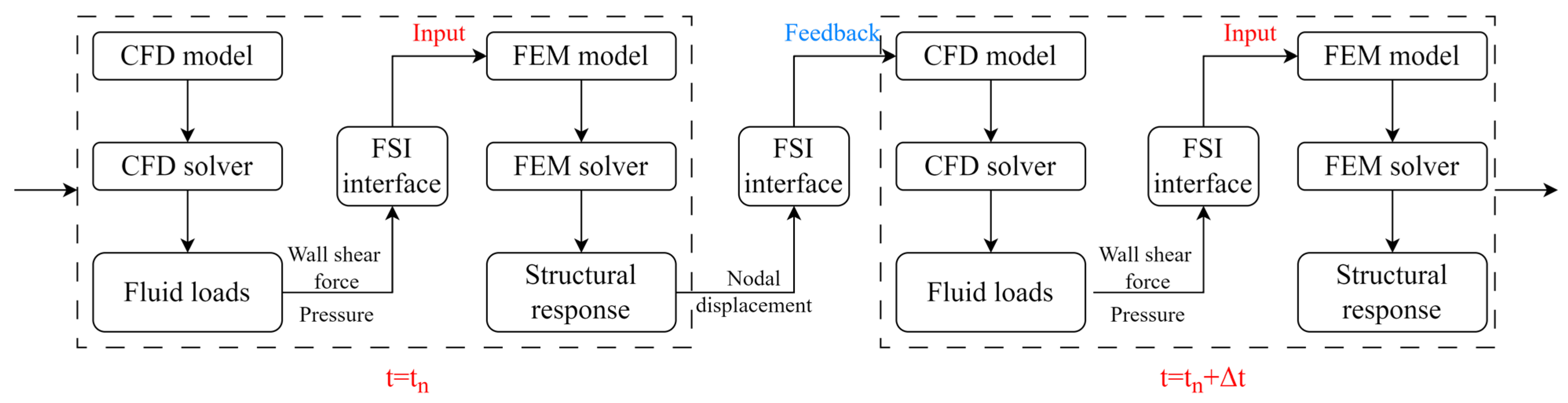
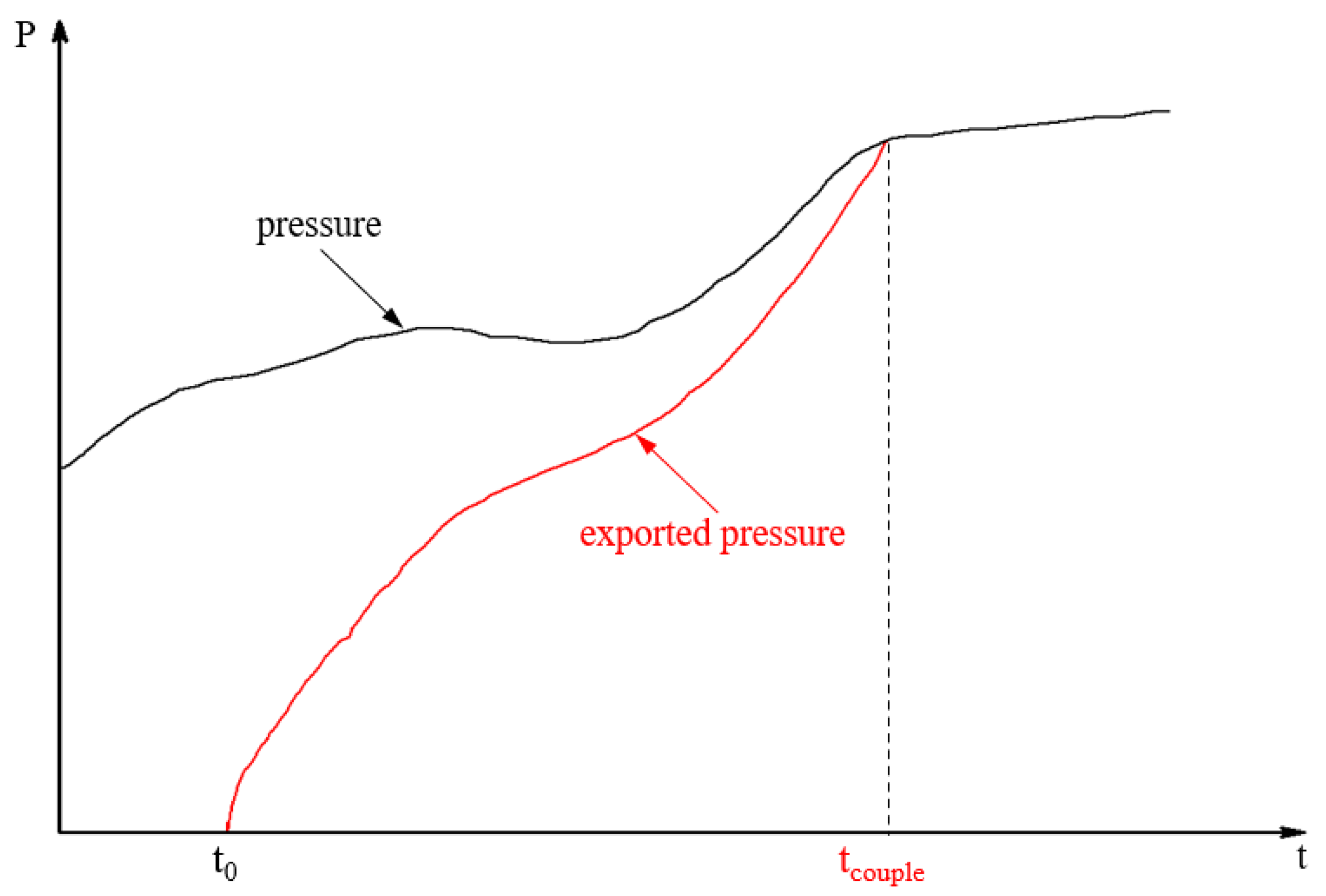
3.3. Co-Simulation Technology

The finite volume method retains data at either the cell center or face center of each individual control volume, and the finite element method records solution data at the nodes of each respective element. In co-simulation, the correlation between the fluid and structural models is determined by their spatial positioning. Since the fluid mesh is not aligned with the structural mesh, an interpolation process using the least squares method is employed to map the fluid pressure onto the structural model. Conversely, when it is necessary to map the displacements of the structure into the flow field, shape functions are utilized for interpolation [22].

The data exchange between the two solvers employs an implicit scheme. The fundamental process of this scheme for solving the coupled Equation (7) is illustrated in Figure 2, demonstrating one data exchange within a single time step. In the initial phase, the fluid solver computes the load based on the initial flow field conditions. This load is then mapped onto the coupling interface of the structural model. The structural solver computes the structural response to this applied load. Upon completion, the nodal displacement data from the coupling interface are transferred back to the fluid solver. Subsequently, the structural boundary within the flow field is updated through mesh deformation, enabling the solution of the flow field for the next time step. It is critical to note that the data exchange process typically requires numerous iterations within a single time step to achieve convergence.

4. Hydroelasto-Plastic Response Analysis for Ship Structures

4.1. Research Object

Due to the expensive computational demands associated with co-simulation calculations, an idealized box girder model representing the ship structure, as shown in Figure 3, is introduced to validate the proposed methodology. The model comprises three holds. The middle hold is considered as the target, and the aft and fore holds are regarded as loading parts. Each hold is 2250 mm in length, 1000 mm in width, and 300 mm in height. The plate thickness in the middle hold is 1.5 mm, whereas in both the aft and fore holds, it is 3 mm. The material adopted is aluminum alloy, and the properties are shown in

Table 1. Properties of material.

Parameter	Value	Unit
Density	2700	Kg/m3
Yield strength	70	MPa
Elasticity modulus	69,000	MPa
Poisson ratio	0.33	-

.

4.2. Numerical Calculation

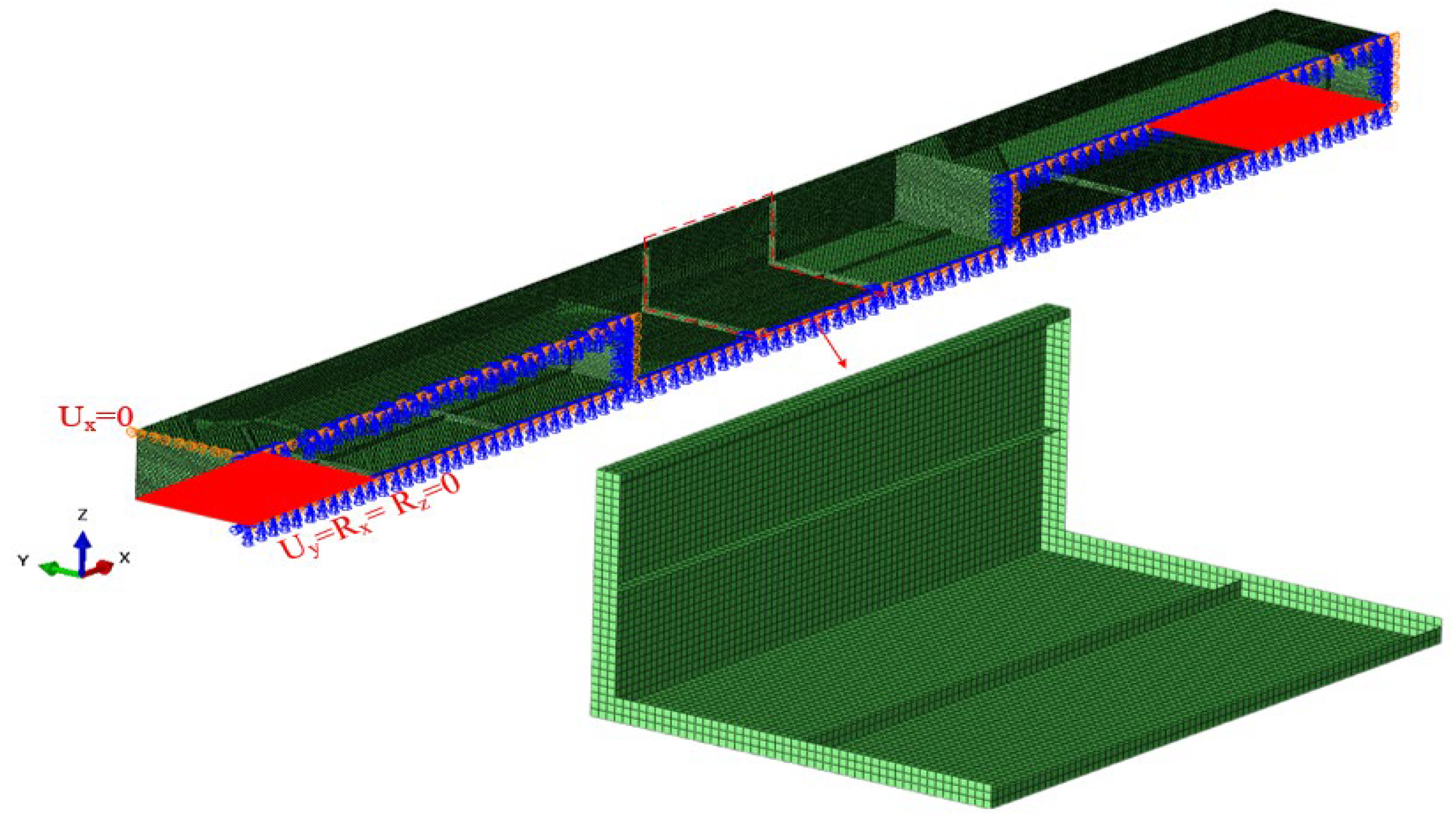
4.2.1. FEM Model

In the structural response analysis, the full structure model employs a uniform mesh size. All elements are defined as ideal elastic–plastic materials, with a structural damping ratio of 2% applied. The nonlinear effects of large deformations and displacements are included in the simulation. Owing to the axisymmetric nature of both the structure and the load, the box girder structure is represented as a half-width model, as shown in Figure 4. This study focuses exclusively on the structural response during a 180° wave encounter. Additionally, the six-degree-of-freedom rigid motion of the model is limited to pitch and heave motions. Therefore, the displacement in the x-direction at the stern of the model, where nodes are located, is restricted. A YSYMM symmetry boundary is applied to the central longitudinal section of the model. For all nodes on this section, the y-direction displacement and rotation around the x- and z-axes are constrained. The model’s structure weighs 62.84 kg. To amplify the elastic–plastic response of the structure to waves, additional ballast is added in the red area within the aft and fore cabins to increase the hydrostatic bending moment. The final total weight of the model reaches 680.34 kg.

To ensure accurate reflection of the structure’s elasto-plastic deformation within the flow field during co-simulation, a highly refined mesh scheme is utilized. Along adjacent longitudinal stiffeners, a total of 25 elements are distributed. Two elements are distributed on the web plate of each longitudinal stiffener, and three elements are distributed on the web plate of each transverse stiffener. The size of the mesh is uniformly set to 10 mm × 10 mm. The hull surface is defined as the FSI interface, as shown in Figure 5.

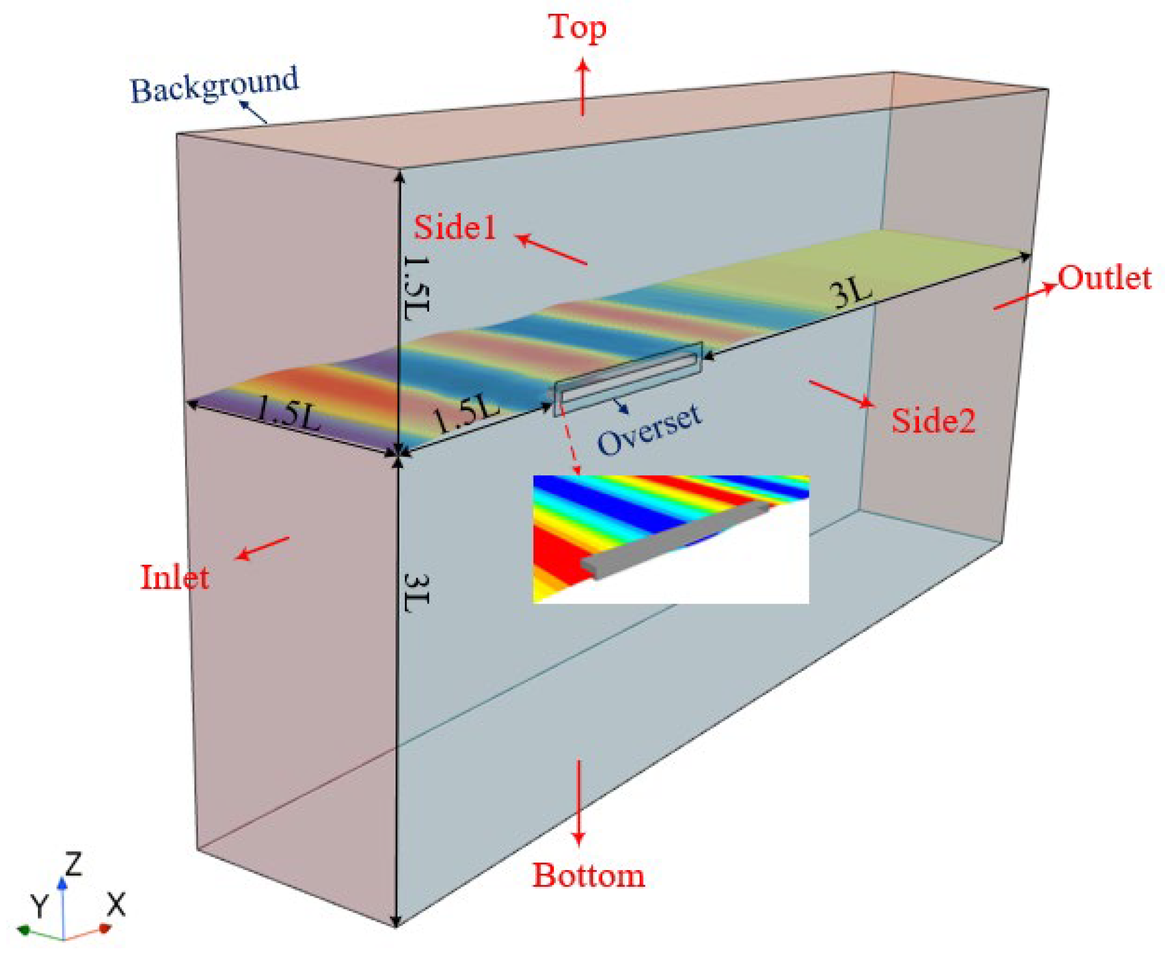
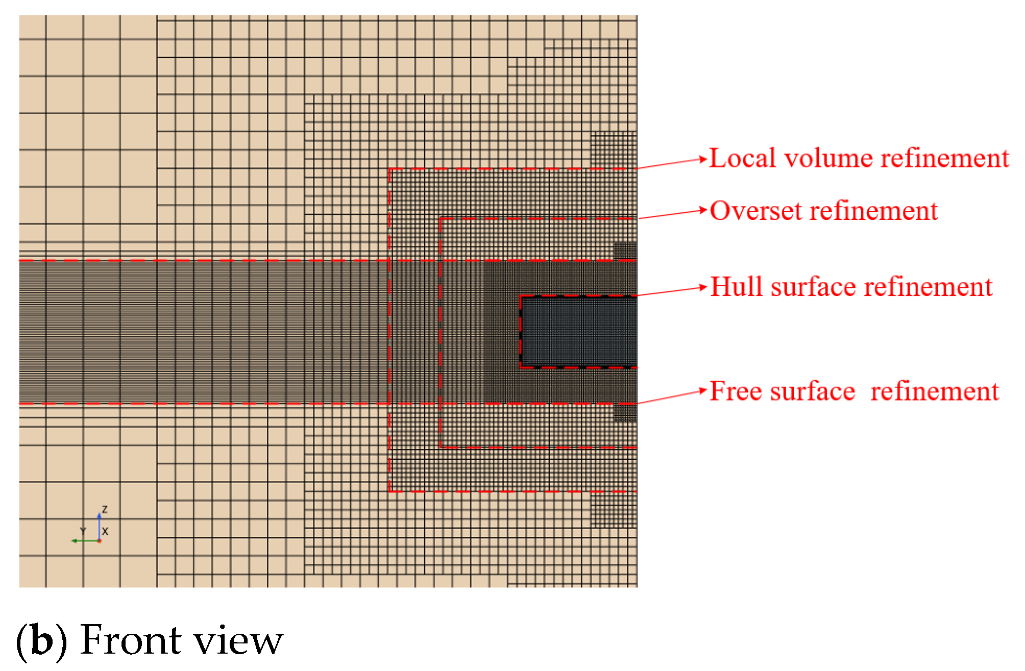
4.2.2. CFD Model

The flow field is partitioned into a background region and an overset region. Encircling the ship hull is the overset region, which exchanges data with the background region through its overset interface. The specific configuration is depicted in Figure 6. “L” denotes the length of the model. The inlet, top, and side 1 boundaries are positioned at distances of 1.5 times the model length ahead, above, and adjacent to the model, respectively. The outlet and the bottom boundaries are placed at 3 times the model length behind and beneath the model, respectively. The inlet boundary is defined as a velocity inlet, where the distributions of velocity and fluid properties are prescribed. Specific conditions are applied to calculate the inlet volume flux, as well as the fluxes of momentum and energy. Both the outlet and the top boundaries are configured as pressure outlets, with the boundary face values of all remaining variables extrapolated from the solution domain’s interior. The bottom, side 1, and the surface of the model boundaries are configured as walls, representing impermeable surfaces that contain fluid or solid regions. For viscous flows, a no-slip condition is implemented at the wall boundary. Consistent with the structural model, a half-width model is employed in the CFD model; therefore, the side 2 boundary is established as a symmetry plane to minimize the computational domain’s extent. In the simulation, the k–epsilon turbulence model is employed to solve transport equations for turbulent eddy viscosity determination. The fifth-order approximation of the Stokes wave theory is used to model wave behavior. This method generates waves with a regular periodic sinusoidal distribution, closely resembling reality and offering a significant improvement over the first-order wave model. To mitigate the impact of wave emission, wave absorption is applied in the region between the model and the outlet boundary.

Due to the fact that large structural deformation can easily lead to non-convergence in fluid load solving, a strict mesh scheme is implemented. The flow field employs a trimmed cell mesher to generate unstructured hexahedral meshes, enabling precise control over mesh generation and localized refinement. Additionally, a prism layer mesher generator is utilized to create boundary layer meshes near the structure surface. In accordance with the guidelines set forth by the ITTC [23], a minimum of 40 elements per wavelength and 16 elements per wave height is required to ensure wave simulation stability. Furthermore, the surface mesh dimensions on the structure within the flow field must closely match those of the structure’s shell mesh in the finite element model. The mesh scheme details are shown in Figure 7. The base mesh sizes in the background and overset regions are 320 mm and 20 mm, respectively. The hull surface mesh size is 10 mm. To ensure fluid mesh quality, the following refinements are applied: local volume refinement outside the overset region, overset region refinement, free surface refinement, and hull surface refinement. The local volume refinement scheme outside the overset region maintains 10 layers of elements in the background domain, which align with the overset boundary mesh size to ensure interpolation accuracy. In this study, the wavelength matches the ship length, and the wave height is 300 mm. The longitudinal span of a standard wavelength contains 168 elements, while the height span contains 30 elements. A boundary layer mesh with a thickness of 5 units is selected.

In the CFD solver, a second-order time discretization scheme is utilized. The time step is set to 0.005 s based on the requirement of the Courant number [24]. To ensure congruence in data transmission between the CFD and FEM solvers at the respective time nodes, the time step for the FEM solver and the coupling exchange time step are also defined as 0.005 s. Convergence is ensured by performing four data exchanges per time step, with the CFD solver executing five internal iterations per exchange. A total simulation time of 4 s is computed, and the process requires approximately 89 h on 48 processors operating at 2.9 GHz.

4.3. Result Analysis

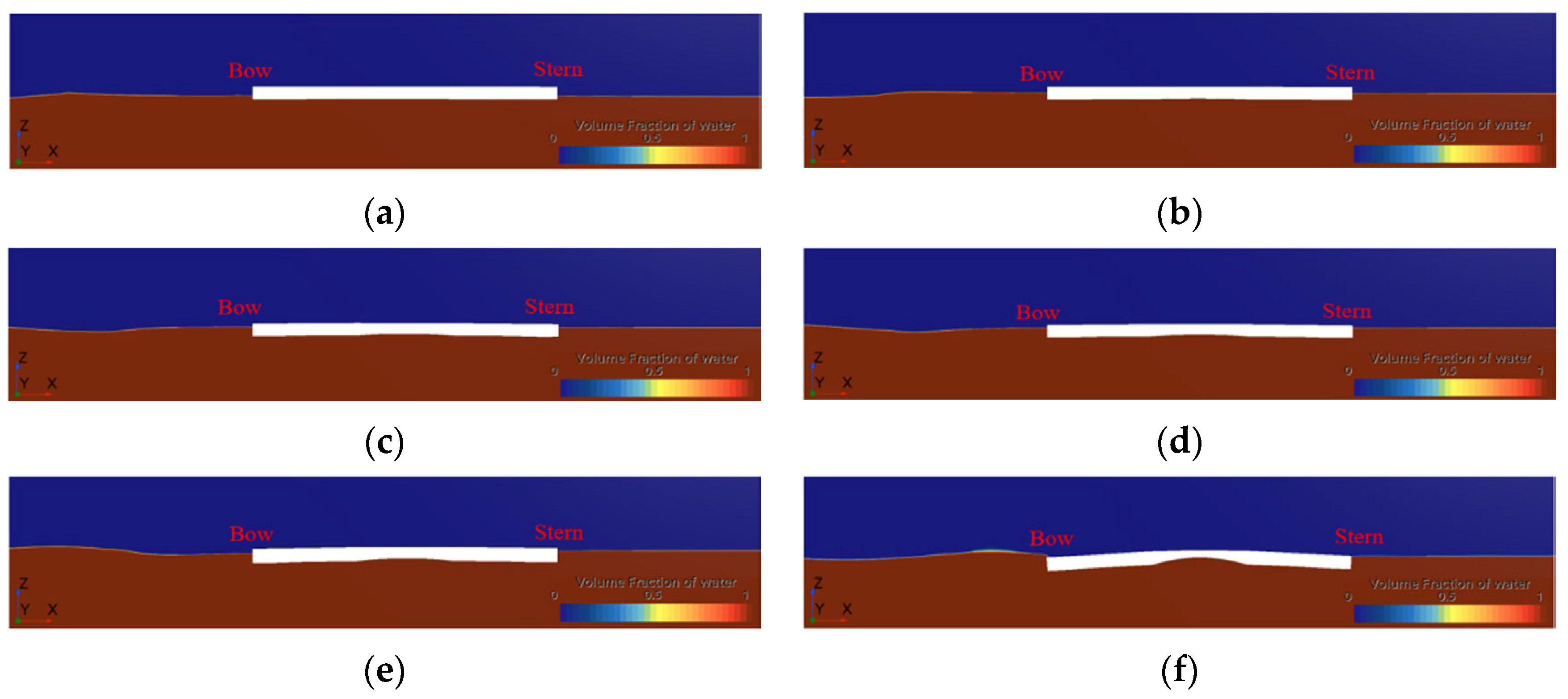
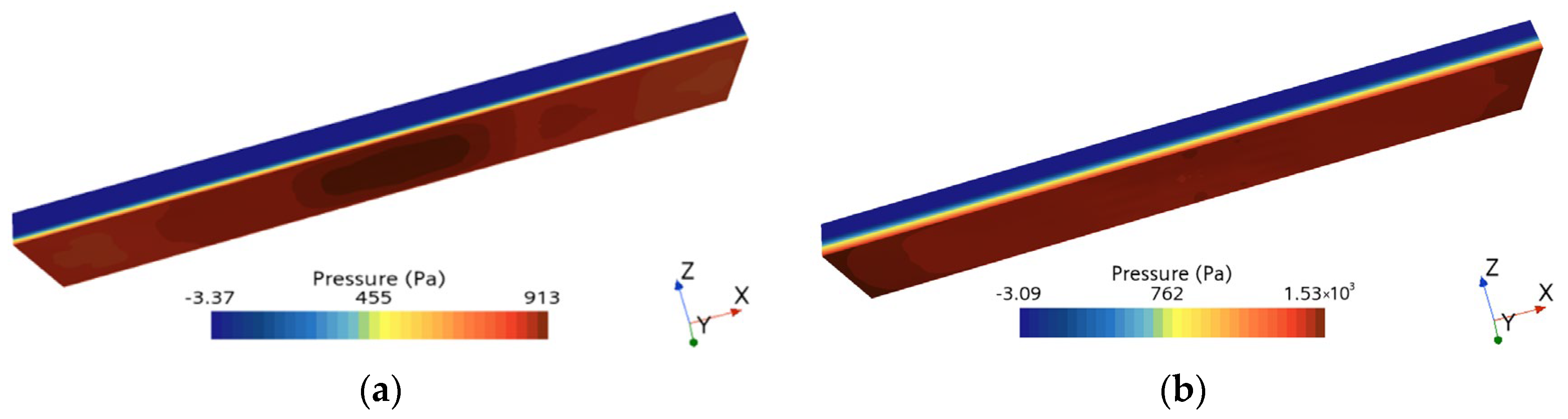
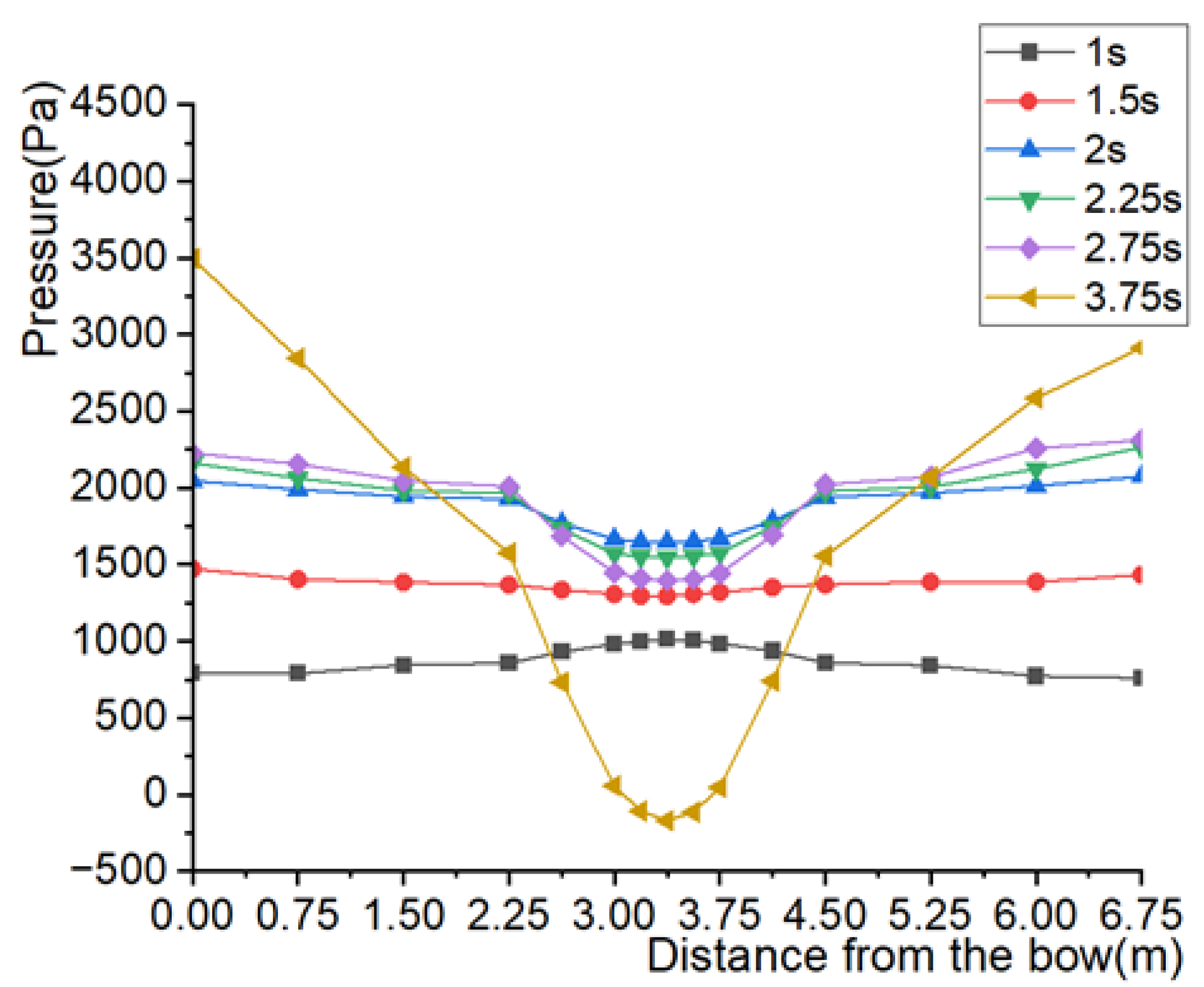
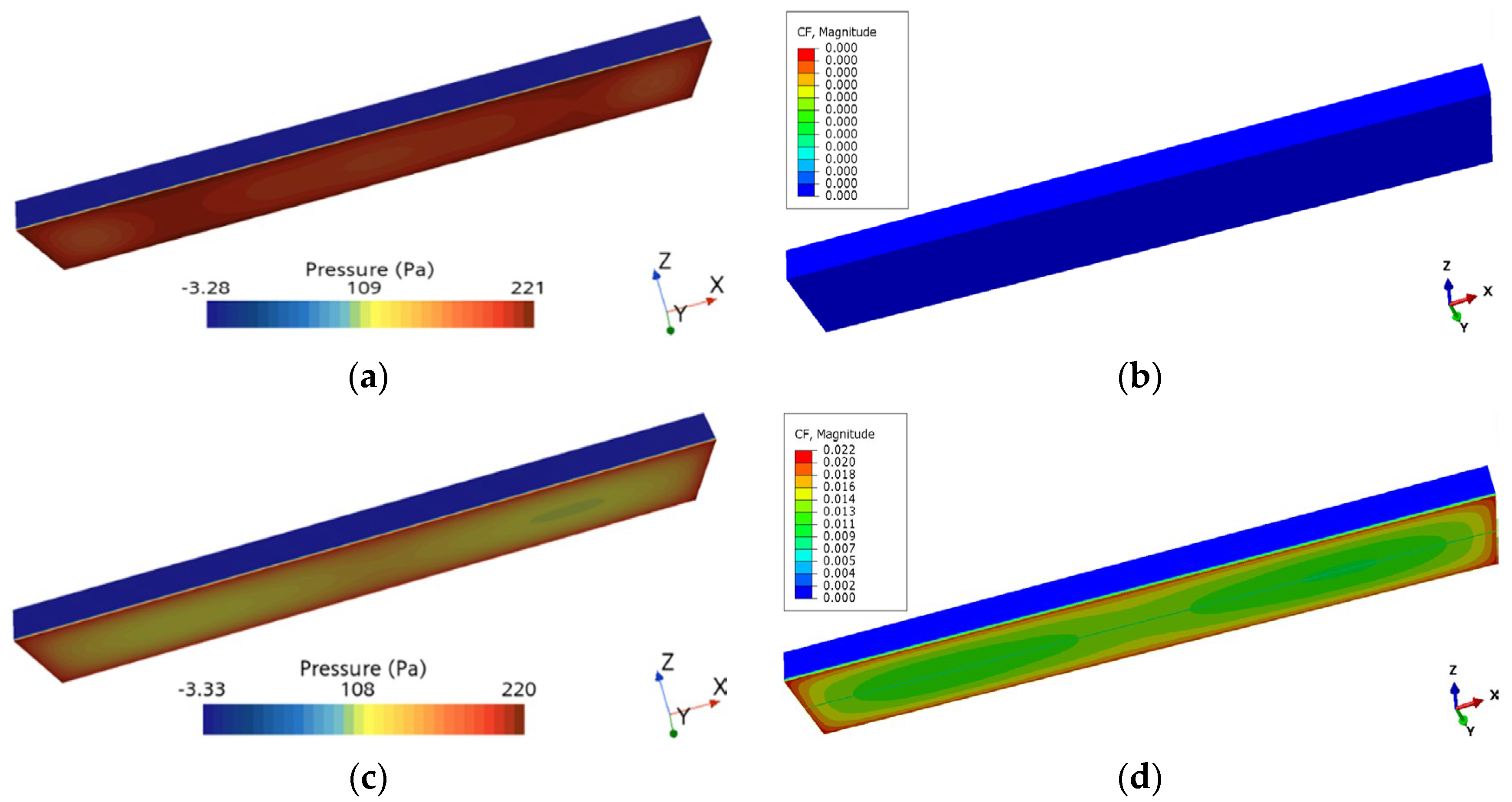
4.3.1. Hydrodynamic Analysis

When a structure undergoes rapid large deformation, the associated added mass disrupts the equilibrium of the dynamic equations, potentially causing numerical divergence. To address this, the ballast mass is gradually increased during the initial calculation phase to ensure a smooth transition from the undeformed state to the force-balanced configuration. The first wavefront is positioned one wavelength ahead of the model bow. The fluid volume fraction distribution of the midship longitudinal section at different time instances is illustrated in Figure 8, with the red and blue regions denoting the water and air phases, respectively. The results demonstrate that incremental ballast loading leads to a proportionally increasing hull draft. As the hydrostatic bending moment rises, the hogging deformation is amplified correspondingly. When wave-induced dynamic loads exceed the structural bearing capacity, collapse occurs, resulting in significantly intensified deformation.

The z-direction displacement response of the whole structure at 2 s is shown in Figure 9. The left is the displacement response of the structure in the FEM solver, and the right is the morpher displacement in the CFD solver. The results show that the structural response can be well considered in the load calculation. Under the combined loads of ballast and water pressure, there is not only overall bending deformation but also localized out-of-plane deformation on the bottom.

The distribution of water pressure along the length of the ship is monitored through 15 measuring points on the ship’s bottom, as depicted in Figure 10. The distance between measurement points in the aft and fore holds remains consistent at 750 mm. Due to the pronounced deformation in the middle hold, the spacing between the measurement points is progressively reduced to 187.5 mm.

The pressure distribution on the hull surface is shown in Figure 11. As the structural draft increases, the water pressure on the hull surface continuously rises. Simultaneously, structural deformations alter the water pressure distribution. Hogging deformation and localized out-of-plane deformations reduce the water pressure in the central region of the ship’s bottom plate while increasing it at both ends. As the deformation degree grows, the disparity in water pressure between the central region and the ends proportionally increases. The bending moment exerted on the structure by the wave gradually intensifies as the wave crest approaches the midpoint of the model, leading to progressive structural deformation. During structural collapse, the sudden increase in deformation causes a significant shift in the water pressure distribution.

In the numerical solution of two-way FSI, the dynamic coupling effect between structural deformation and the fluid pressure field can induce non-physical numerical oscillations in the fluid domain solution. This is especially pronounced during the system’s initial non-equilibrium stage, as shown in Figure 12. At t = 1 s, the water pressure in the central area of the bottom exceeds that at both ends, contradicting physical reality. However, as the iterative algorithm progresses and the structural displacement increment satisfies the convergence tolerance, the coupling system’s energy dissipation mechanism becomes predominant. Consequently, the condition number of the Jacobian matrix for the flow field pressure Poisson equation improves, effectively suppressing decoupling errors between the continuity and momentum equations.

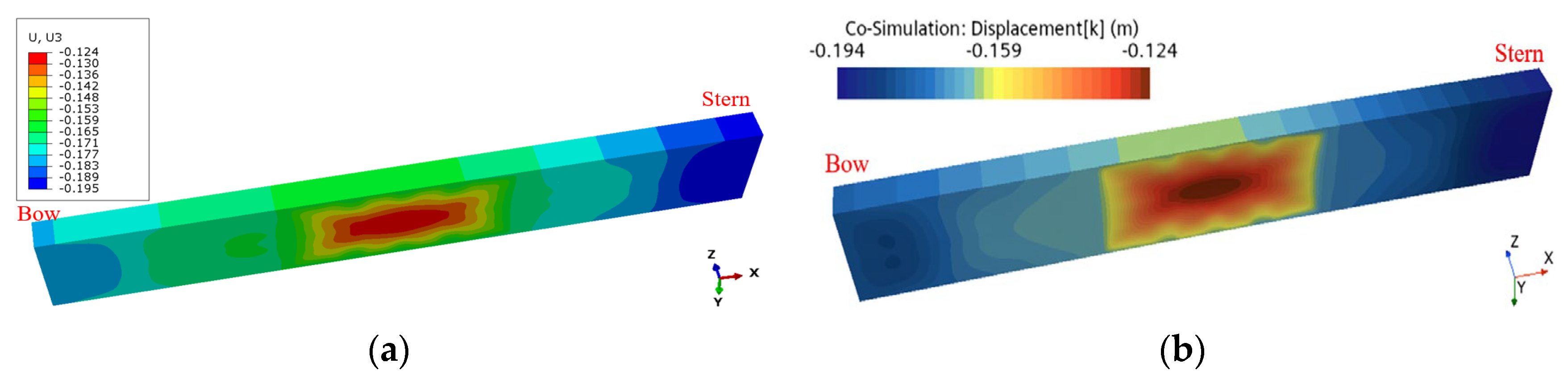
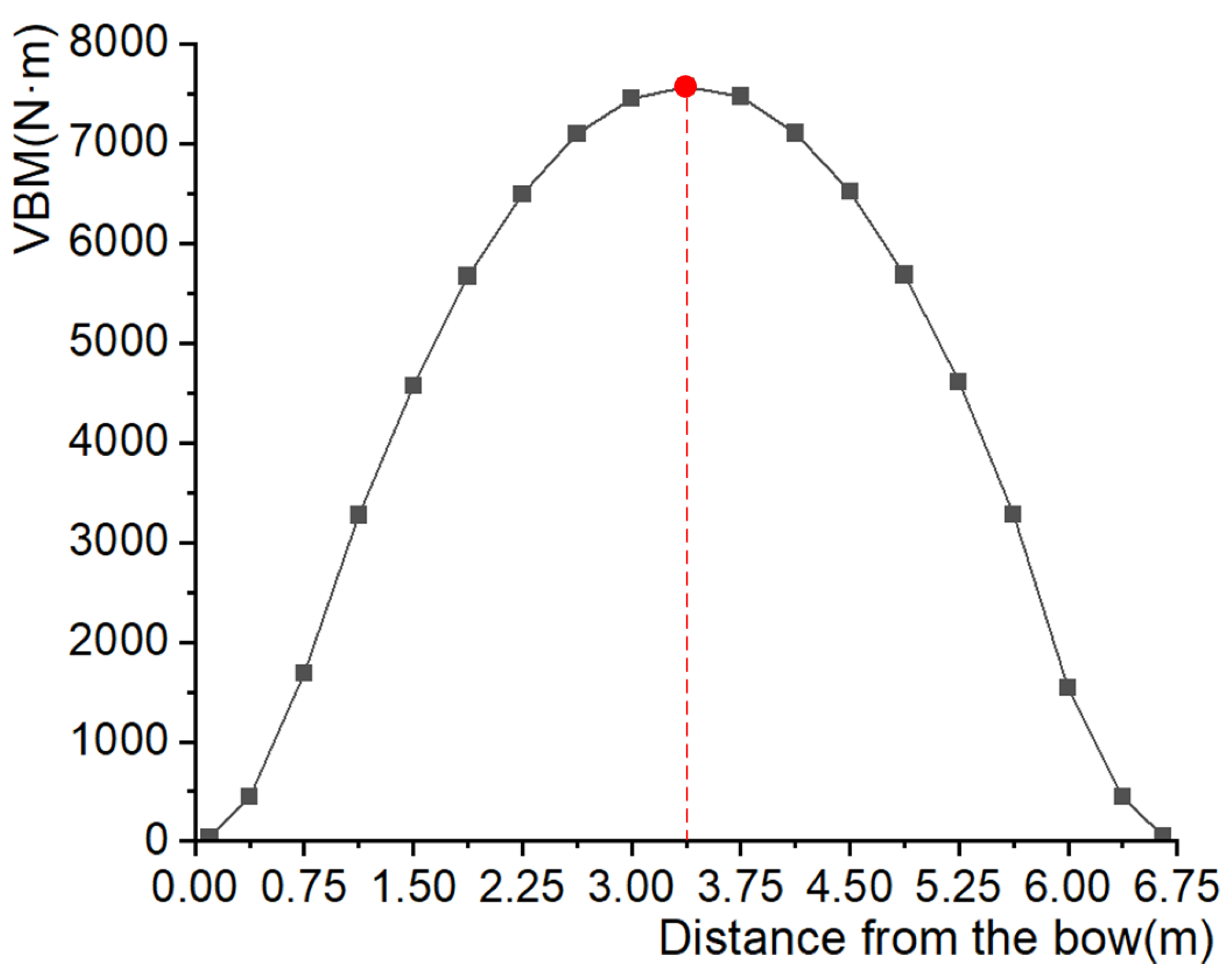
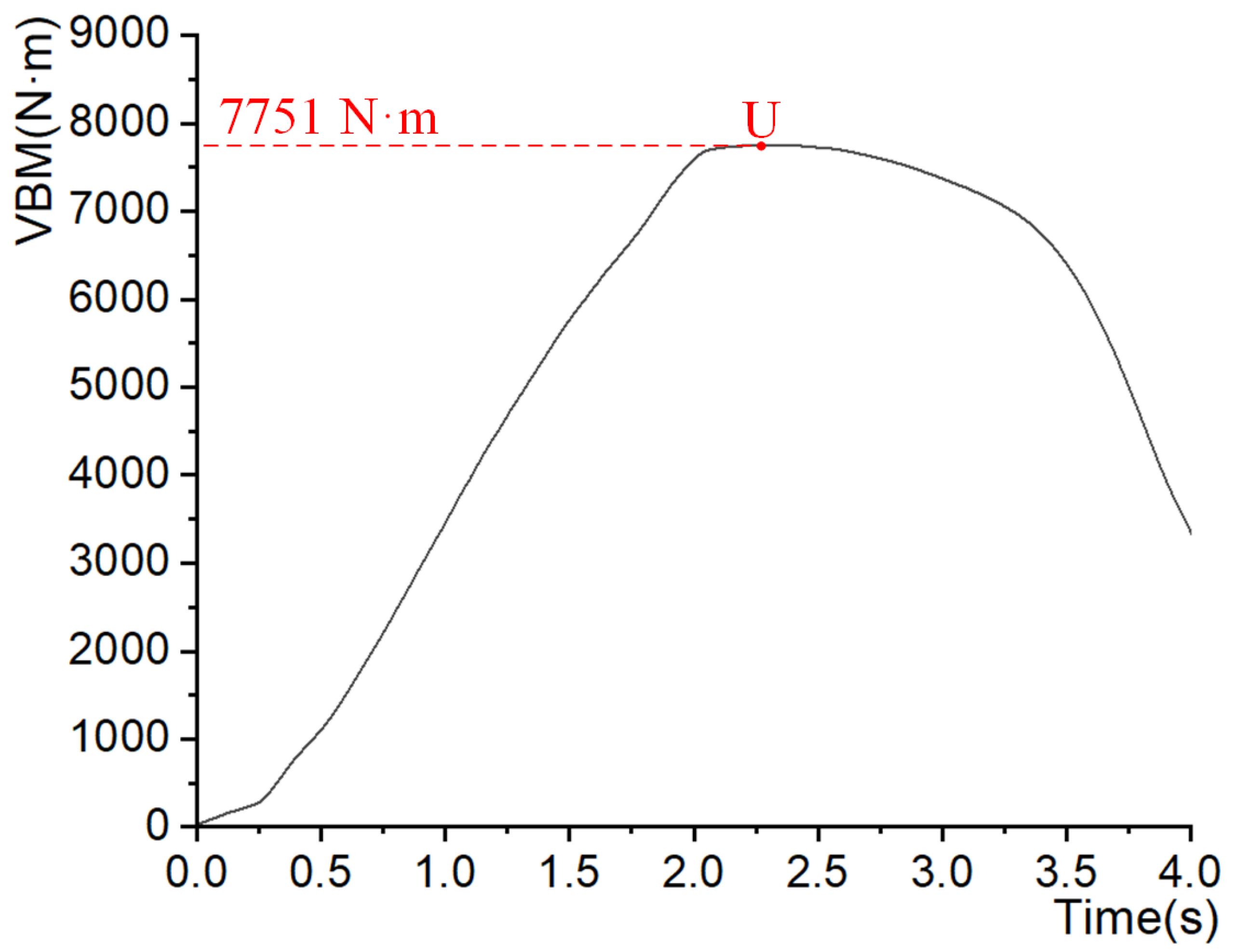
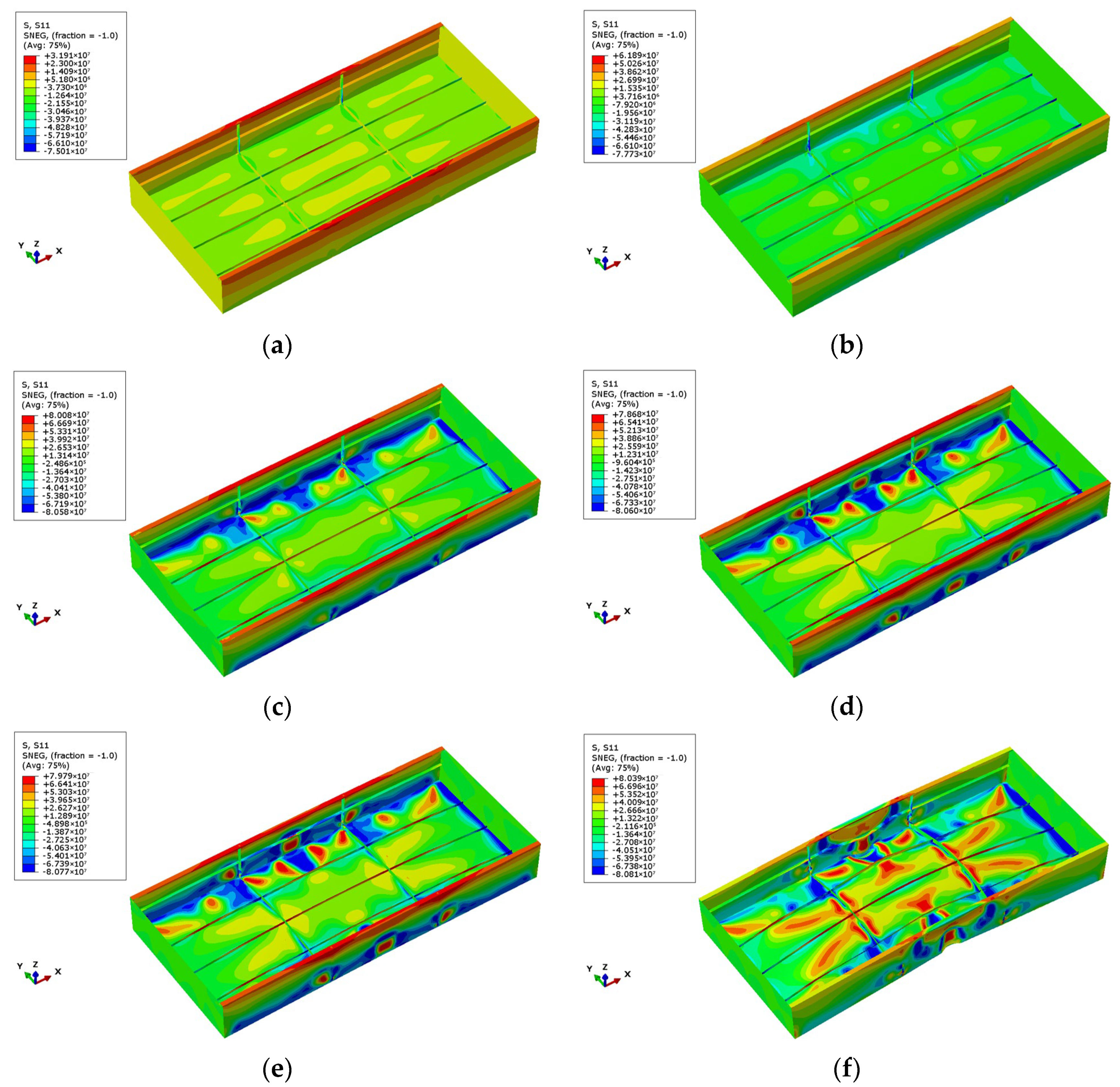
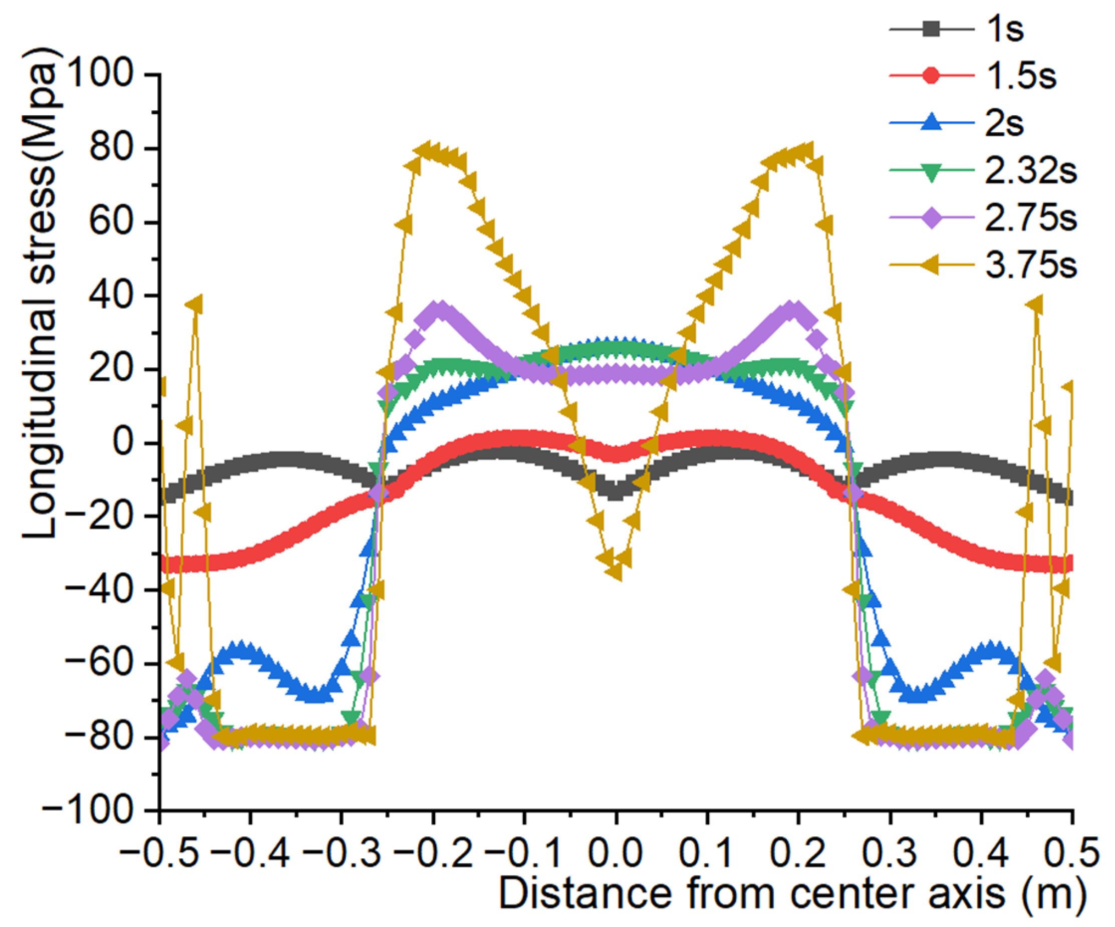
4.3.2. Progressive Collapse Behavior Analysis

In the initial stage, it is critical to progressively apply the pressure calculated by the CFD solver to the structure to ensure numerical stability. This is achieved by carefully adjusting the exported traction field, as shown in Figure 13. The abscissa represents the CFD solver’s computational timeline, where t₀ and t_couple denote two manually specified coupling instances, and the ordinate corresponds to the load magnitude. The black curve indicates the actual hydrodynamic load calculated in the CFD simulation, while the red curve represents the load transferred to the FEM solver. At the beginning of the simulation, the structure remains unloaded, and the CFD solution provides the initial flow field for the independent rigid body analysis. When t < t₀, the CFD solver exports zero force. For t₀ < t < t_couple, the exported force gradually converges to the calculated value. Once t exceeds t_couple, the exported force fully matches the calculated force. In this study, t₀ and t_couple were set to 0 s and 0.2 s, respectively. The pressure computed by the CFD solver and imported into the FEM solver at 0.2 s is illustrated in Figure 14, where loads are applied as nodal concentrated forces.

The VBM (vertical bending moment) distribution along the model length at t = 2 s is shown in Figure 15. Due to the combined effects of gravity and buoyancy, the structure exhibits a hogging deformation state, resulting in the maximum bending moment occurring in the midship section, with significantly smaller values at the ends. The time history of the VBM in the midship section is illustrated in Figure 16. The results demonstrate that the bending moment gradually increases as ballast is added and the draft deepens. Before t = 0.2 s, the bending moment rate remains low because the fluid load applied to the structure is intentionally ramped up slowly. After t = 0.2 s, the rate of increase accelerates markedly. By t = 2 s, the structure approaches its ultimate load-bearing state. Upon wave impact with the model at t = 2.32 s, the surge in the wave-induced bending moment drives the structure to reach its ultimate state, with a recorded peak bending moment of 7751 N·m. Subsequently, the structure undergoes gradual unloading, causing a reduction in the bending moment. When the structural bearing capacity is entirely depleted, the bending moment drops rapidly.

The longitudinal stress distribution of the middle hold with a large opening at typical moments is shown in Figure 17. When the ballast is small, the sheer strake experiences tensile stress under the hogging bending moment, while the bottom plate undergoes compressive stress. Localized out-of-plane deformation occurs in the plating between the bottom keels due to water pressure, leading to reduced stress in those regions. As the load increases, the structural stress intensifies. Adjacent to the bilge, the structures transition into a plastic state under compressive loads, whereas the sheer strake yields plastically under tension, resulting in a gradual reduction in the structure’s load-bearing capacity. When the plating near the bilge exhibits significant buckling deformation, the overall structure reaches its ultimate state. Beyond this point, the failure zone continues to expand under persistent loading, though residual load-bearing capacity remains. As local out-of-plane deformation intensifies, the longitudinal keel undergoes tripping, further degrading its load-bearing performance. Even after the wave-induced bending moment diminishes, structural deformation rapidly accelerates once the bearing capacity is entirely lost.

The longitudinal stress distribution of the side plate in the midship transverse section is illustrated in Figure 18. At t = 1 s and t = 1.5 s, under shallow draft conditions, the longitudinal stress shows a linear distribution across the depth. As the draft increases to a critical threshold, localized out-of-plane deformations aligned with the lateral water pressure direction develop in the bilge-adjacent plating of the side plate, triggering a transition in stress state from compression to tension in this region. Subsequently, under combined bending moment and localized water pressure effects, the out-of-plane deflection amplitude gradually amplifies, leading to elevated stress levels. Concurrently, the plating above the side keel undergoes reverse out-of-plane deformations, shifting from an initial tensile state to a compressive state. The longitudinal stress distribution of the bottom plate is shown in Figure 19. Under small external loads, the bottom plate is in global compression. Subjected to vertical water pressure, out-of-plane deformations with uniform orientation occur on both sides of the bottom longitudinal keels, causing localized stress reduction at the plating center. As external loads further increase, the direction of out-of-plane deformation reverses in the plating between the side keel and the bilge, resulting in a significant stress increase within this region. Stress variations in the plating between adjacent side keels remain relatively small. Oppositely oriented out-of-plane deformations on either side of the side keels induce tripping of the keels, progressively diminishing structural stability and ultimately causing collapse.

5. Conclusions

In this study, a hydroelasto-plastic analysis methodology was proposed and applied to a collapse analysis of an idealized box girder representing ship structures. This method can integrate load calculations with structural response analyses, thereby considering the coupling effect. Through the analysis of the load distribution and the progressive collapse behavior, the mechanism of FSI is revealed, yielding the following conclusions:

1.

The CFD-FEM co-simulation methodology enables a two-way coupled analysis of elasto-plastic structural deformation and hydrodynamic load through iterative exchange of the load and structural response data within a small time step, thereby providing a robust solution framework for elasto-plastic structural response analysis under wave actions.

2.

The structural response not only passively reflects the effects of fluid loads but also actively modifies the flow field characteristics and boundary conditions, thereby reconfiguring the spatiotemporal distribution of hydrodynamic loads. When structural responses are significant, their influence on fluid loading becomes pronounced. Therefore, FSI effects must be incorporated into the analysis of ship hull structural responses under wave actions to ensure accurate load predictions and integrity assessments.

3.

Ship structures exhibit a local structural response under the action of out-of-plane water pressure, and this affects the overall structural progressive collapse process. The method presented in this paper not only considers the FSI effect but also considers the local structural response, thus improving the ability to clarify the wave-induced collapse mechanism of marine structures.

4.

In future research, model experiments will be conducted to validate the accuracy of the proposed methodology. Furthermore, full-scale actual ship structural collapse mechanisms under marine environmental loads will be systematically investigated based on this approach, aimed at providing critical technical support for hull structural safety design and lightweight optimization strategies.

References

- Cinquini, C.; Venini, P.; Nascimbene, R.; Tiano, A. Design of a river-sea ship by optimization. Struct. Multidiscip. Optim. 2001, 3, 240–247. [Google Scholar]
- Shi, G.; Wang, D. Ultimate strength model experiment regarding a container ship’s hull structures. Ships Offshore Struct. 2012, 7, 165–184. [Google Scholar]
- Wang, C.; Wu, J.; Wang, D. Experimental and numerical investigations on the ultimate longitudinal strength of an ultra large container ship. Ocean Eng. 2019, 192, 106546. [Google Scholar]
- Wang, Q.; Wang, C.; Wu, J.; Wang, D. Experimental and numerical investigations of the ultimate torsional strength of an ultra large container ship. Mar. Struct. 2020, 70, 102695. [Google Scholar]
- Wang, Q.; Wang, D. Warping and shear behaviors involved in hull girder’s torsional collapse process. Thin-Walled Struct. 2020, 157, 107123. [Google Scholar]
- Lee, D.H.; Paik, J.K. Ultimate strength characteristics of as-built ultra-large containership hull structures under combined vertical bending and torsion. Ships Offshore Struct. 2020, 15, S143–S160. [Google Scholar] [CrossRef]
- Pei, Z.; Yuan, Q.; Ao, L.; Wu, W. A research on similarity law for combined ultimate bending and torsional strength. Ships Offshore Struct. 2023, 19, 1254–1265. [Google Scholar]
- Lehmann, E. Discussion on “Report of committee III. 1: Ultimate strength”. In Proceedings of the 16th ISSC (3), Southampton, UK, 20–25 August 2006; pp. 121–131. [Google Scholar]
- Xiao, T.; Fan, J.; Mei, G.; Hou, G.; Chen, L.; Zhang, C.; Hu, M. Strength analysis of overall ship FEM model based on design wave approach. Ship Sci. Technol. 2010, 32, 14–19. (In Chinese) [Google Scholar]
- Pei, Z.; Iijima, K.; Fujikubo, M.; Tanaka, S.; Okazawa, S.; Yao, T. Simulation on progressive collapse behaviour of whole ship model under extreme waves using idealized structural unit method. Mar. Struct. 2015, 40, 104–133. [Google Scholar]
- Bishop, R.E.D.; Price, W.G.; Tam, P.K.Y. Unified dynamic analysis of ship response to waves. Nav. Archit. 1977, 6, 363–390. [Google Scholar]
- Bishop, R.E.D.; Price, W.G.; Temarel, P. A unified dynamic analysis of antisymmetric ship response to waves. RINA Trans. 1979, 112, 349–365. [Google Scholar]
- Wu, Y.; Price, W.G. A general form of interface boundry condition of fluid-structure interaction and its application. Sel. Pap. Chin. Soc. Nav. Archit. Mar. Eng. 1985, 1, 66–87. [Google Scholar]
- Iijima, K.; Yao, T.; Moan, T. Structural response of a ship in severe seas considering global hydroelastic vibrations. Mar. Struct. 2008, 21, 420–445. [Google Scholar] [CrossRef]
- Ni, X.; Cheng, X.; Lu, Y.; Wu, B.; Wang, Q.; Zhang, K.; Yu, J. Evaluation of hydroelastic responses of a 180k DWT large bulk carrier. Ocean Eng. 2020, 199, 106948. [Google Scholar] [CrossRef]
- Lakshmynarayanana, P.A.; Temarel, P. Application of a two-way partitioned method for predicting the wave-induced loads of a flexible containership. Appl. Ocean Res. 2020, 96, 102052. [Google Scholar] [CrossRef]
- Jiao, J.; Huang, S.; Soares, C.G. Viscous fluid–flexible structure interaction analysis on ship springing and whipping responses in regular waves. J. Fluids Struct. 2021, 106, 103354. [Google Scholar] [CrossRef]
- Iijima, K.; Kimura, K.; Xu, W.; Fujikubo, M. Hydroelasto-plasticity approach to predicting the post-ultimate strength behaviour of ship’s hull girder in waves. J. Mar. Sci. Technol. 2011, 16, 379–389. [Google Scholar] [CrossRef]
- Iijima, K.; Fujikubom, M. Hydro-elastoplastic behaviour of VLFS under extreme vertical bending moment by segmented beam approach. Mar. Struct. 2018, 57, 1–17. [Google Scholar] [CrossRef]
- Liu, W.; Song, X.; Pei, Z.; Li, Y. Experiment study of hydroelasto-buckling ship model in a single wave. Ocean Eng. 2017, 142, 102–114. [Google Scholar] [CrossRef]
- Liu, W.; Luo, W.; Yang, M.; Xia, T.; Huang, Y.; Wang, S.; Leng, J.; Li, Y. Development of a fully coupled numerical hydroelasto-plastic approach for offshore structure. Ocean Eng. 2022, 258, 111713. [Google Scholar] [CrossRef]
- STAR-CCM+, Version 8.0; Software for Computational Fluid Dynamics; Manual; Siemens: Munich, Germany, 2012.
- ITTC. Recommended Procedures and Guidelines: Practical Guidelines for Ship CFD Applications; ITTC: Zürich, Switzerland, 2011. [Google Scholar]
- Lakshmynarayanana, P.A.; Temarel, P. Application of CFD and FEA coupling to predict dynamic behaviour of a flexible barge in regular head waves. Mar. Struct. 2019, 65, 308–325. [Google Scholar]