Computational Fluid Dynamics Analysis of Ballast Water Treatment System Design

Abstract

The effective management of ships’ ballast water is critical for preventing the spread of invasive species. Despite advancements in UV-based ballast water treatment systems (BWTSs), achieving a uniform flow distribution within UV reactors (UVRs) remains challenging due to the spatial constraints of ships. This study employs computational fluid dynamics (CFD) to analyze turbulent seawater flow in a real-case BWTS installed on a self-discharging bulk carrier. The flow uniformity at UVR inlets and the volume flow rate (Q) distribution between parallel reactors are evaluated at nominal flow rates of 1000, 1900, and 2000 ${\mathrm{m}}^3/\mathrm{h}$. The results indicate significant disparities at maximum capacity (2000 ${\mathrm{m}}^3/\mathrm{h}$), with the starboard configuration exceeding the recommended Q per UVR by 4.95%, thus requiring operational adjustments. Six geometric modifications are assessed, revealing that optimized pipeline bends and T-junction designs (e.g., ST_3 and ST_4) improve velocity uniformity and maintain the relative Q distribution errors below 8.5%. This study identifies vortical structures generated by sharp geometrical transitions as primary contributors to flow instability. By bridging CFD insights with practical engineering constraints, this work provides feasible recommendations for retrofitting existing BWTSs and designing future systems, ultimately enhancing treatment efficacy, reducing UV lamp wear, and supporting compliance with International Maritime Organization (IMO) standards.

1. Introduction

The global marine ecosystem is facing mounting environmental challenges, with the management of ships’ ballast water emerging as a critical concern for ocean health. Global maritime trade grew by 2.4% in 2023, reaching 12,292 million tons, with more than 80% of world trade carried by sea despite challenges at key chokepoints like the Suez and Panama Canals due to geopolitical tensions, conflicts, and climate change [1]. To maintain stability and ensure safe navigation, vessels must take on ballast water when operating with partial or no cargo. This essential practice has become a significant environmental concern as maritime trade expands, introducing invasive species and harmful microorganisms that irreversibly alter marine biodiversity and cause substantial ecological and economic repercussions [2]. Although species transfer occurs through various vessel components such as hull fouling [3], sea chests [4], and anchors [5,6], ballast water presents the greatest risk due to its substantial volumes. The transportation of harmful microorganisms through ballast water, sediments, and tank biofilms [7] has led to widespread ecological disruption, with research indicating that invasive species affect 84% of global ecosystems [8]. The establishment of invasive aquatic species presents a persistent ecological challenge, as their introduction is practically irreversible, and their environmental impact tends to intensify over time [9]. Moreover, these species spread not only through larger intercontinental distances but also through regional dispersal within local seas [10], amplifying their ecological footprint. These biological invasions profoundly impact food webs, water quality, and human health [11]. The discharge of ballast water not only threatens marine ecosystems but also imposes substantial economic burdens on affected regions [12,13,14].

To address these environmental, health, and economic challenges, the International Maritime Organization (IMO) adopted the “International Convention for the Control and Management of Ships’ Ballast Water and Sediments” in 2004 [15], establishing strict limits on organism concentrations in discharged ballast water. The convention mandates that all ballast water treatment systems (BWTSs) must receive approval from competent flag state authorities [16], with additional IMO approval required for systems utilizing active substances to ensure ship safety and protect both human health and aquatic environments [17]. The evolution and implementation of these ballast water management regulations, as comprehensively documented by Campara et al. [18], have led to the development of various physical and chemical treatment methods as efficient solutions for onboard ballast water treatment.

BWTSs primarily utilize chlorination, ozonation, and ultraviolet (UV) irradiation, with UV-based systems employing medium-pressure lamps and UV-induced advanced oxidation processes. The effectiveness of UV disinfection relies on biomolecules, particularly nucleic acids, absorbing UV energy, which causes structural modifications to genetic material and subsequently inhibits cell replication. The inactivation efficiency depends on specific parameters, including wavelength selection, radiation dosage, and environmental conditions, especially the presence of substances that may reflect or absorb UV radiation. Comprehensive reviews have extensively documented the technological evolution, challenges, and solutions in BWTSs over the years [19,20,21,22,23,24,25].

In the past 10 years, several studies have conducted in-depth analyses of ballast water treatment, especially focusing on UV reactors (UVRs). The study in [26] examined six BWTSs divided into two categories: UV radiation and chlorine disinfection. The UV-based systems utilized varying configurations of UVRs and light sources, with all systems demonstrating similar patterns of phytoplankton reduction to levels below IMO limits. Petersen et al. [27] revealed bacterial regrowth in ballast water following both UV and electrochlorination treatments. Their study demonstrated that bacterial activity serves as a more reliable indicator of treatment efficiency than bacterial density measurements, as original bacterial populations, including potential pathogens, can reestablish when favorable nutrient conditions emerge post-treatment. Pecarevic et al. [28] combined a hydrocyclone (HC) for sediment removal and initial organism inactivation with subsequent UV radiation for final seawater sterilization. Two studies [29,30] investigated several different methods and techniques to meet the IMO’s ballast water discharge standards for the 10–50 μm size class and check UVR performance. To optimize UVR performance and address the current inefficiencies in BWTSs, the study in [31] developed an advanced control system. Most of today’s UVRs in commercial systems operate with basic ON/OFF controls, often running at full capacity regardless of water flow, resulting in an unstable UV dosage, excessive energy consumption, and a reduced lamp lifespan.

Among the reviewed literature, only Thach et al. [31] employed computational fluid dynamics (CFD) to analyze the flow field at the UV reactor’s inlet. Similarly, Joo et al. [32] studied the flow through the UV reactor for BWT, though with minimal inlet and outlet piping. Zhang et al. [33] provided a comprehensive chemical analysis of BWT samples, but their CFD analysis was limited to the UV reactor’s flow field. While these studies have significantly advanced the understanding of BWT, practical challenges remain in distributing BWT components within confined engine rooms. For UV-based systems, analyzing pipeline systems, particularly between the filter and UV reactor, is crucial. However, CFD analysis of the fluid flow in BWT systems remains understudied. This research presents the first detailed CFD investigation of the pipe fluid flow in a real-case scenario featuring two UV reactors in a parallel arrangement. This study examines ballast water treatment units (BWTUs) installed on both the port and starboard sides of a newbuilding self-discharging bulk carrier’s engine room, focusing on the turbulent water flow characteristics. The key objectives include verifying flow uniformity through the pipeline system, especially at the UV reactor entrance, and ensuring a proper flow distribution between the reactors to prevent exceeding their volume flow rate capacity.

This paper comprises four sections. Section 2 outlines the BWTS layout for the port and starboard sides, including simplified 3D models for CFD simulations and numerical analysis methods. Section 3 presents a computational analysis of pipeline flow fields, focusing on the UV reactor inlet volume flow rates and flow uniformity. This section also explores potential geometric modifications to improve the flow characteristics within the constraints of the engine room space. Finally, Section 4 offers concluding remarks and recommendations for optimizing BWTS pipeline designs in confined spaces.

2. Problem Description and Methodology

The ship’s ballast water treatment system (BWTS) consists of two treatment units (BWTUs) installed on the port and starboard sides of the engine room. Each BWTU features two UV reactors in a parallel arrangement. Proper BWTU operation requires a balanced flow distribution to prevent exceeding the capacity of individual UV reactors. The BWTS provides a total nominal capacity of 4000 ${\mathrm{m}}^3/\mathrm{h}$, with each BWTU handling 2000 ${\mathrm{m}}^3/\mathrm{h}$. CFD analysis precedes operational testing to verify system safety and compliance with flag state requirements, providing valuable insights for BWTU manufacturers, shipyard contractors, and ship owners.

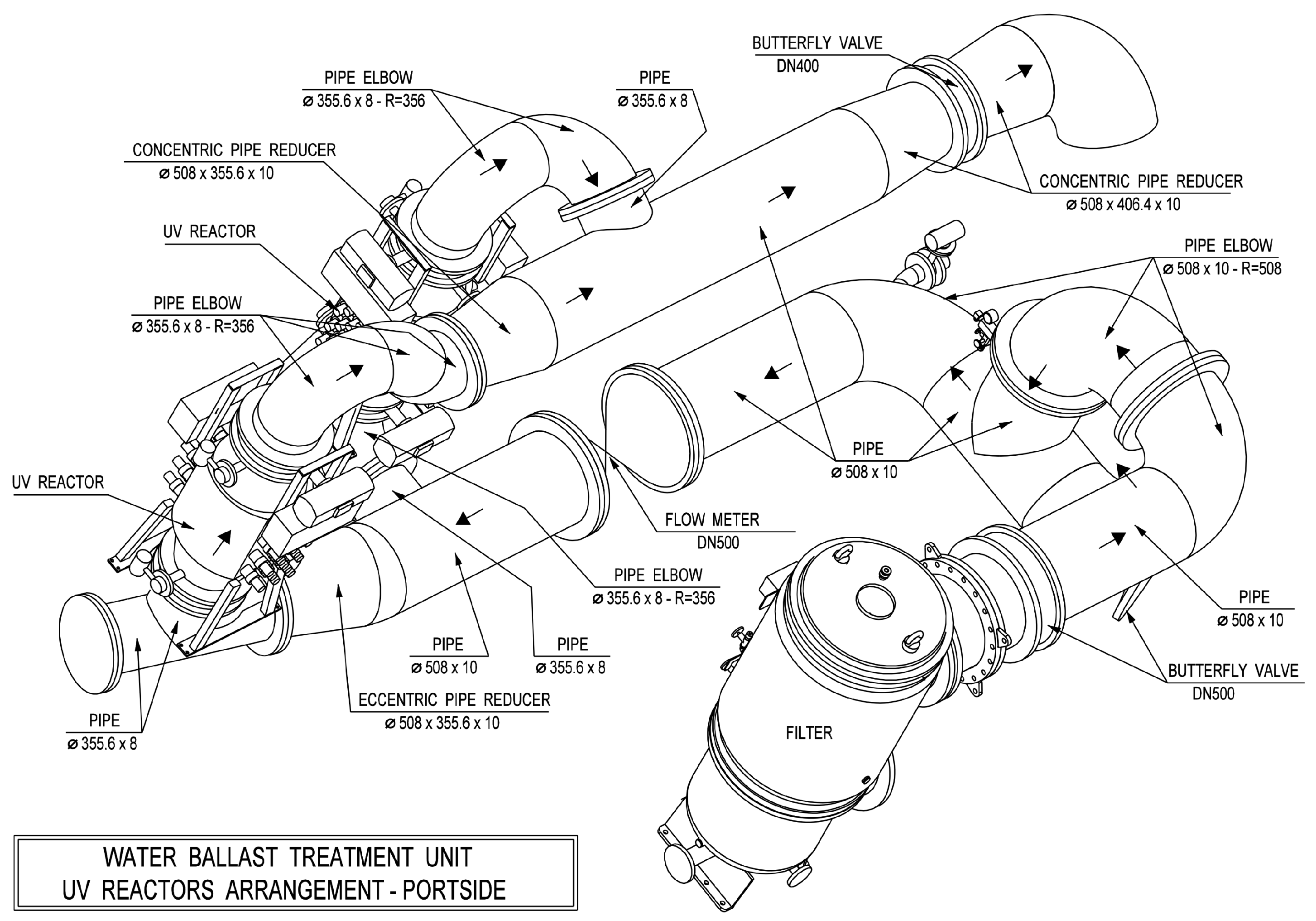
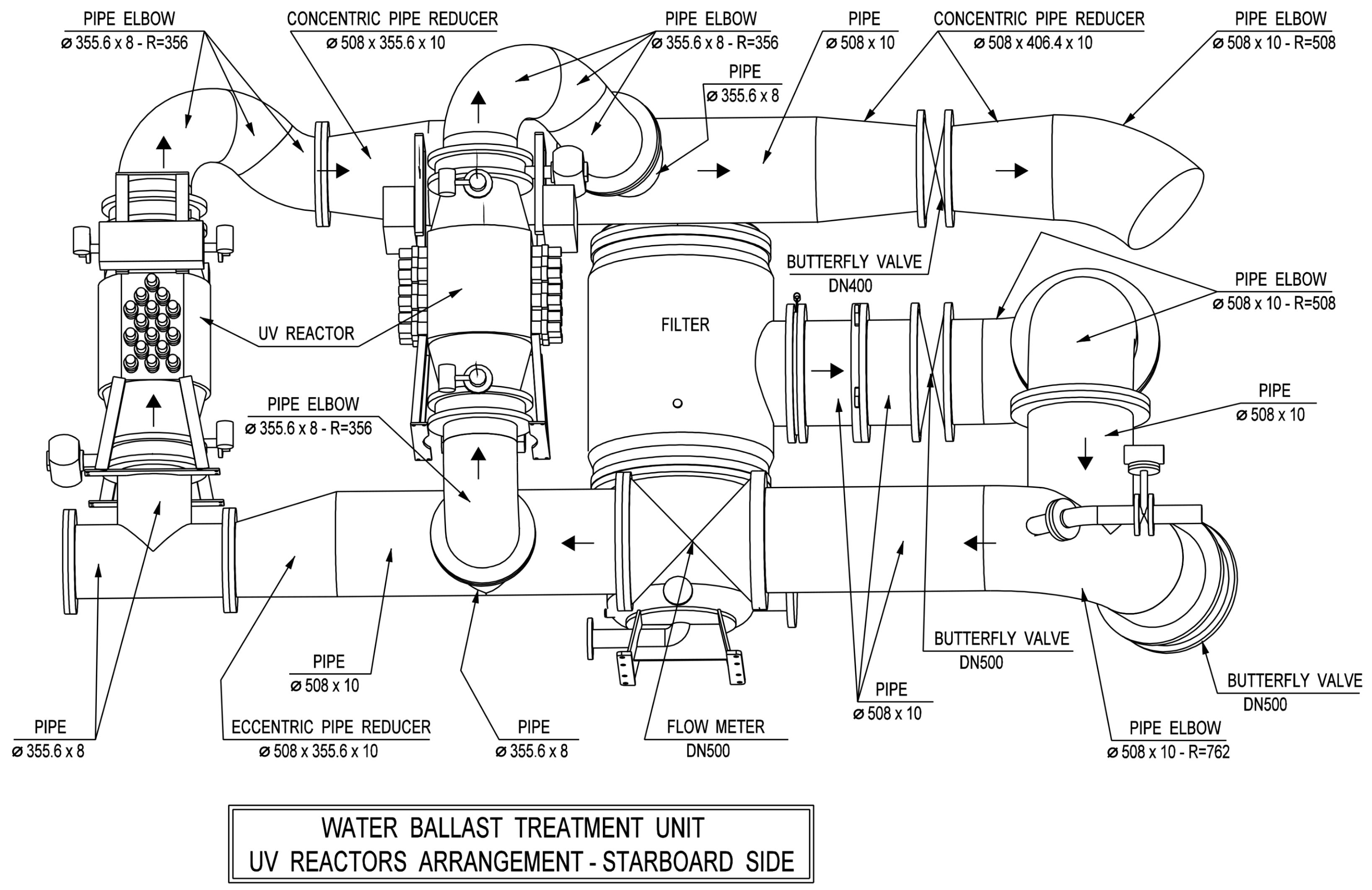
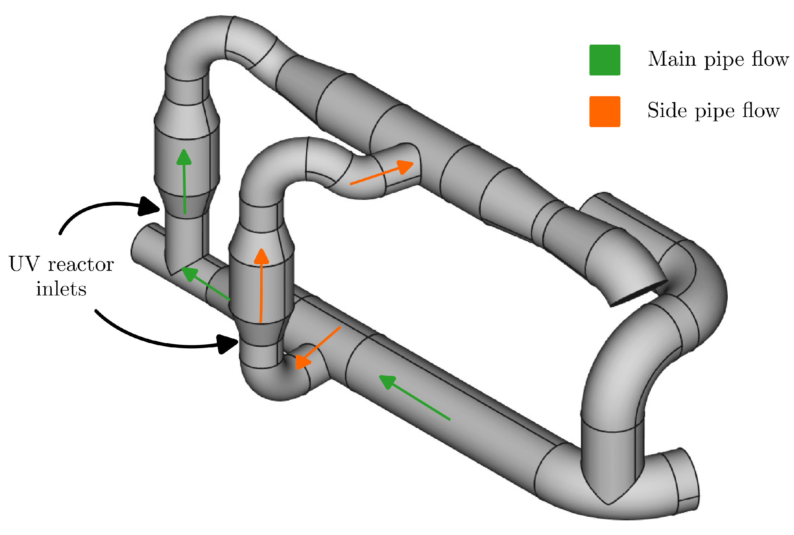
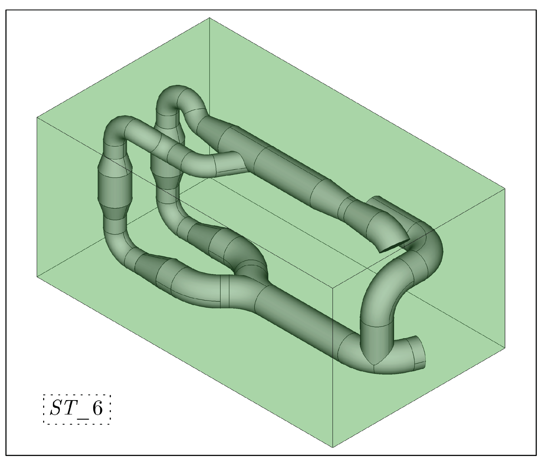
2.1. Ballast Water Treatment System (BWTS) Layout

Pipeline and equipment installation follows the manufacturer’s requirements within the available engine room space. Two critical considerations specified by the manufacturer for equipment installation and CFD simulation are as follows:

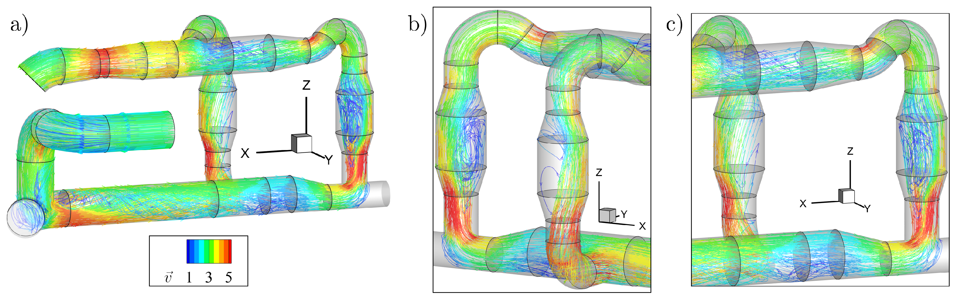
• Opposing flow directions in the inlet and outlet manifolds connected to the UV reactors.
• Extending the CFD domain from the filter outlet to at least three pipe diameters $(3·d)$ downstream of the last UV reactor.

The second point is particularly crucial for CFD analysis, as the wall near the outlet may influence pipe flow. To mitigate this effect, a minimum distance of $(3·d)$ must be maintained. In both the port and starboard pipeline layouts, this requirement is exceeded, with the distance between the outlet and the point where the side pipe section connects to the main pipe section measuring approximately $(4·d)$. Figure 1 and Figure 2 illustrate detailed arrangements of the port and starboard ballast water treatment systems, which feature similar layouts and identical UV reactors, while Figure 3 and Figure 4 provide 3D models prepared for CFD analysis.

To perform a CFD analysis of the BWTU, 3D CAD models of the pipelines and equipment were created, taking into account the diameters and wall thicknesses of each section of the pipeline. The 3D CAD model included UV reactors and all piping downstream from the filter, including all bends, reductions, and T-junctions, extending a minimum of three pipe diameters beyond the final UVR. For computational efficiency, flanges, flow meters, and UV reactor internals were simplified as cylindrical pipes. The models represent only fluid domains, unlike the complete assemblies shown in Figure 1 and Figure 2. Watertight 3D geometries were generated in FreeCAD using parametric Python macro-scripts to gather all pipeline segments, as illustrated in Figure 3.

Gray cylinders represent the pipe inner diameters. Likewise, internal monitoring surfaces were created within the fluid domain and used in Section 2.2. The port-side model excludes the final elbow near the outlet due to its sharp bend angle, which could compromise numerical stability. This simplification is justified, as the pipe length after the second UVR already satisfies the analysis requirements.

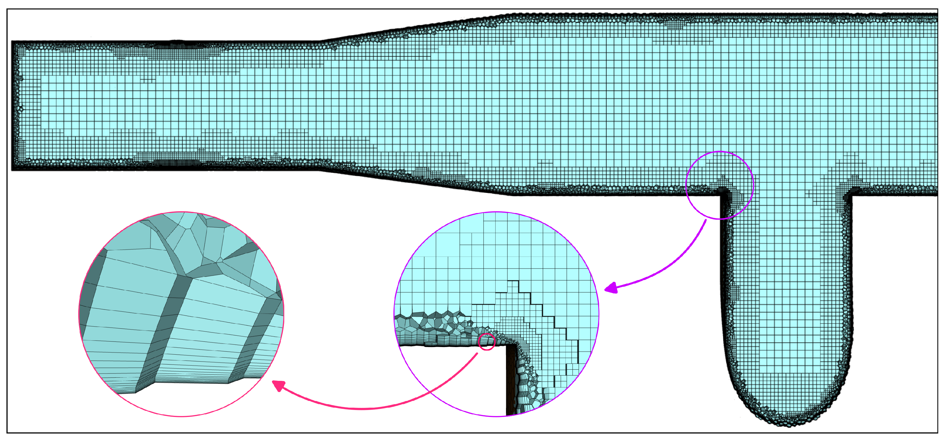
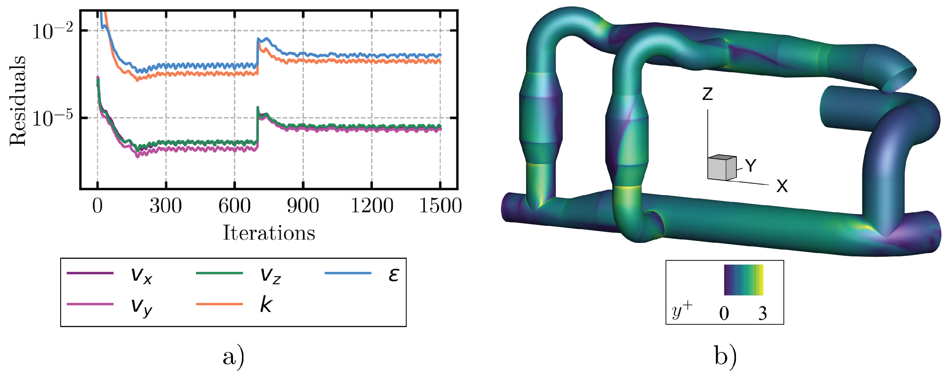
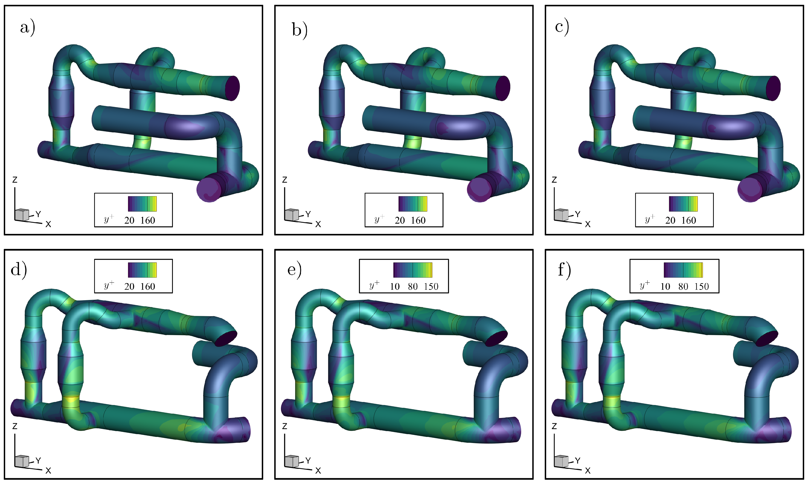
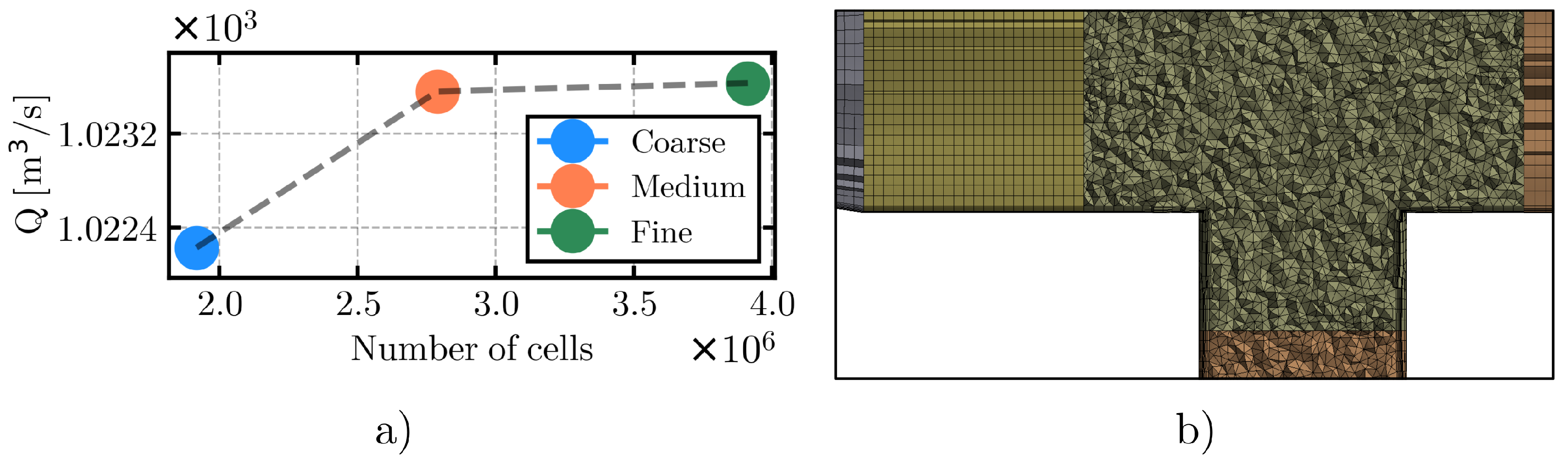
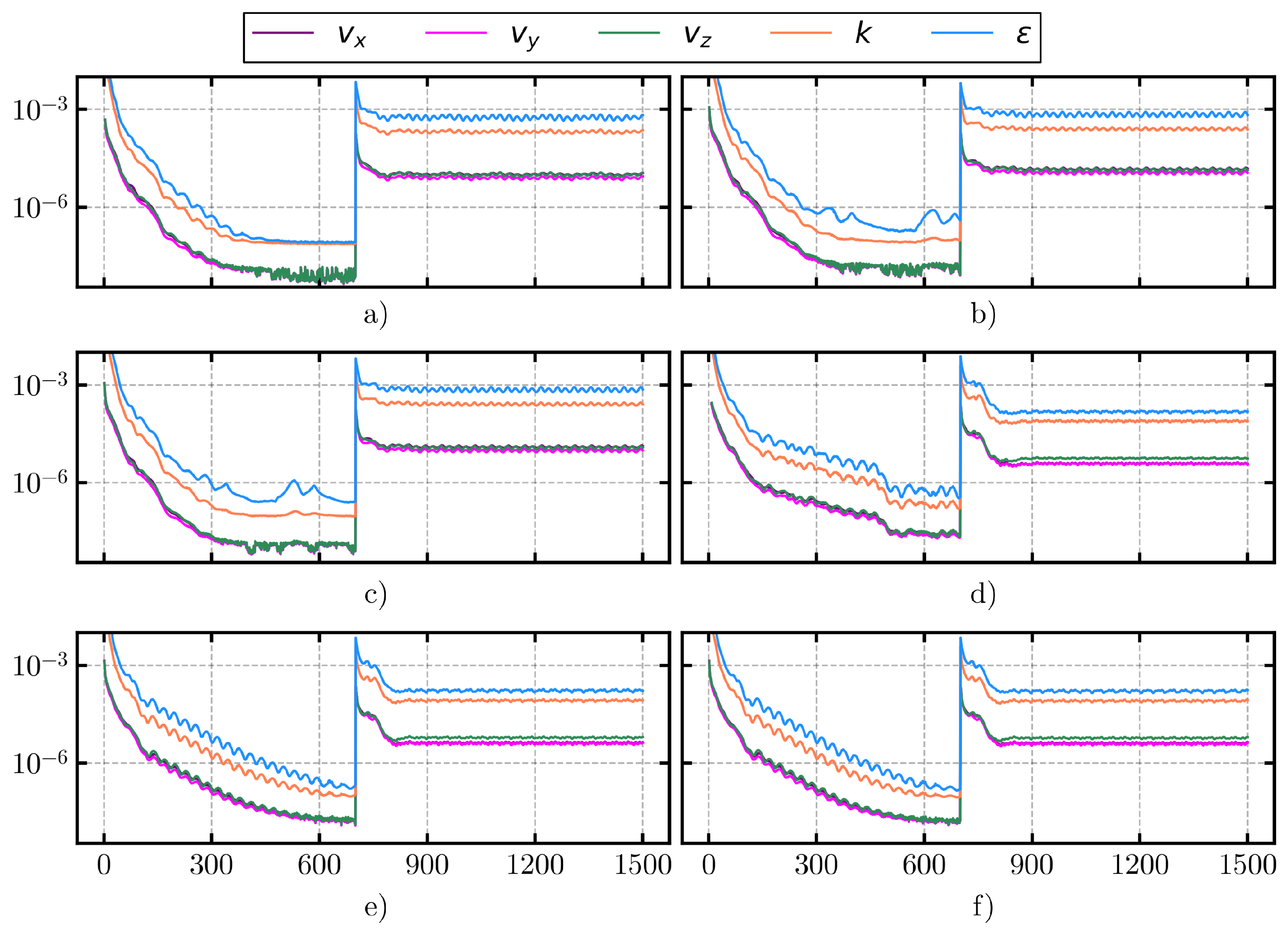
2.2. Numerical Model

Simulations were conducted starting from the filter, which represents the domain’s inlet, using flow rates of 1000, 1900, and 2000 ${\mathrm{m}}^3/\mathrm{h}$ for both the port and starboard configurations. These nominal flow rates were selected for specific reasons. The 2000 ${\mathrm{m}}^3/\mathrm{h}$ case is critical, as it represents the maximum discharge capacity per UV reactor. Ideally, the flow should be distributed equally between the parallel paths and their UV reactor inlets shown in Figure 4. However, an equal distribution is often not achieved due to the turbulent nature of the flow, pressure drops, and energy losses. To address this, a nominal flow rate of 1900 ${\mathrm{m}}^3/\mathrm{h}$ was introduced to comply with the manufacturer’s requirement that each UV reactor should operate below 1000 ${\mathrm{m}}^3/\mathrm{h}$, as discussed in Section 3. Finally, a flow rate of 1000 ${\mathrm{m}}^3/\mathrm{h}$ was simulated to assess whether reducing the nominal flow by half significantly influences the fluid flow characteristics.

The BWTS 3D simulation of fluid flow was performed with the following physical properties of seawater, which were selected according to the given design conditions at 30 °C:

• Density: $\rho =1022{\mathrm{kg}/\mathrm{m}}^3$.
• Kinematic viscosity: $\nu =8.51\times {10}^{-7}{\mathrm{m}}^2/\mathrm{s}$.
• Dynamic viscosity: $\mu =0.87\times {10}^{-3}\mathrm{Pa}·\mathrm{s}$.

The steady-state simulation employs Reynolds-Averaged Navier–Stokes (RANS) equations with a coupled scheme in ANSYS Fluent using the realizable $k–ϵ$ turbulence model with a wall function balances computational cost and speed with numerical efficiency. A more detailed analysis of different turbulent models and mesh setups is discussed in Appendix A. The unstructured mesh combines hexahedral elements for straight pipe sections with tetrahedral elements for elbows, reductions, and T-junctions. The base element size is set to 1/20th of the pipe diameter, with local refinement in complex geometrical features. The mesh density balances simulation accuracy with computational cost, resulting in 2.5–3 million cells per case. The wall function approach requires $y^{+}$ values between 30 and 300. Figure 5 demonstrates compliance with this range across all cases, except for a negligible region near the inlet dead end.

To ensure accurate results, several mesh quality metrics were analyzed. Skewness was maintained below 0.75, and orthogonal quality remained above 0.25 across all cases. In addition to the previously mentioned $y^{+}$ analysis, a grid sensitivity study was performed by comparing the volume flow rates at the main UV reactor inlet for the port-side layout using three mesh resolutions: coarse (1.9 million cells), medium (2.8 million cells), and fine (3.9 million cells), as shown in Figure 6a. All three meshes had similar coarseness change ratios between pipe segments. Inflation layers were constructed using hexahedral elements for the whole BWTS. Regular hexahedral elements were applied in straight cylindrical segments, while T-junctions and elbows were meshed with tetrahedral and pyramid elements featuring finer cell allocation. Although most segments employed hexahedral cells, tetrahedral elements dominated overall (67%) due to their dense distribution in bends and T-junctions, followed by hexahedral (31%) and pyramid elements (2%). Figure 6b visually illustrates the combination of different mesh types on an XY-plane cross-sectional cut of the pipeline’s lower section. The most critical parameter for evaluating the results is the volume flow rate at the UV reactor inlet, particularly within the main pipe section where higher flow values occur. Therefore, a comparison was conducted in this region (Figure 6a), revealing a strong correlation among all mesh densities, especially between the medium and fine resolutions. The relative error in the volume flow rate between the coarse and medium meshes was 0.13%, while that between the medium and fine meshes was only 0.007%. The medium mesh was selected for subsequent simulations, as it provided an optimal balance between accuracy and computational cost.

Simulations proceeded for 1500 iterations with second-order pressure discretization. The momentum, turbulent kinetic energy $\left(k\right)$, and turbulent dissipation rate $\left(ϵ\right)$ spatial discretization transitioned from first- to second-order upwind at iteration 700. Figure 7 shows the resulting residual behavior, where higher-order schemes exhibit characteristic oscillations reflecting flow turbulence.

Solution convergence is achieved with velocity vector residuals reaching ${10}^{-5}$, while the turbulent kinetic energy $\left(k\right)$ and turbulent dissipation rate $\left(ϵ\right)$ stabilize at ${10}^{-3}$ for the starboard side and at ${10}^{-4}$ for the port side. Residual patterns indicate a higher turbulence intensity in the starboard configuration. Flow turbulence induces velocity and turbulence parameter oscillations in the converged solution. The final results represent the averaged values from the last 25% iterations, ensuring a stable representation of the flow characteristics.

3. Results and Discussion

This section presents the results of the current pipeline distribution in a newbuilding and examines how various geometric modifications affect the pipeline uniformity and fluid flow distribution between the UVRs. In Section 3.1, the existing pipeline distribution is evaluated in terms of flow uniformity and its alignment with the manufacturer’s specifications. Section 3.2 compares six additional numerical simulations incorporating different geometric changes that adhere to the available free space in the engine room. These pipeline shape optimizations are assessed using multiple visualization techniques.

3.1. Pipeline Analysis in Newbuilding Engine Room

The primary objectives of this analysis are to examine the turbulent nature of the flow before seawater enters the UV reactors and to calculate the volume flow rate through each UV reactor. The analysis is conducted for both the port- and starboard-side BWTUs at a nominal flow rate of 2000 ${\mathrm{m}}^3/\mathrm{h}$ and a reduced flow rate of 1000 ${\mathrm{m}}^3/\mathrm{h}$. Additionally, due to the volume flow rates approaching the threshold values, a simulation with a nominal flow rate of 1900 ${\mathrm{m}}^3/\mathrm{h}$ is included. The turbulent seawater flow in the port-side BWTU pipeline is visualized using streamlines, as shown in Figure 8.

By comparing the three different volume flow rates, it is evident that the flow directions remain largely consistent across the cases. After seawater passes through the first two elbows and the large T-junction, a dominant vortical structure forms, extending through the longest straight pipe in the system and gradually weakening downstream. In the main pipe section, the flow decelerates due to bifurcation between the main and side pipes, followed by acceleration after the pipe reduction. A smaller T-junction near the UVR inlet introduces a dead-end region, which generates increased turbulence and backflow in the domain. Additionally, at higher flow rates, more chaotic flow enters the narrow pipe leading to the UVR inlet, with higher velocity values observed along the outer edge. The maximum velocity in the system at an inlet volume flow rate of 2000 ${\mathrm{m}}^3/\mathrm{h}$ is 7.51 m/s, while it decreases to 7.13 m/s at a reduced flow rate of 1900 ${\mathrm{m}}^3/\mathrm{h}$. Within the UVR of the main pipe flow, turbulent behavior is observed near the inner edge, while higher velocity values with a more uniform flow are present along the outer edge. It should be noted that the UVRs are modeled as empty (i.e., without UV lamps) to enhance visualization and better understand how pipeline construction influences flow uniformity. In real-world applications, these vortical structures would be mitigated by UV lamp layouts; however, achieving a more uniform flow at the UVR inlet reduces the likelihood of UV lamp damage. The side pipe layout exhibits a similar flow distribution within the UVR but introduces an additional challenge due to the abrupt 90° change in the flow direction from the main pipe to the side pipe. This transition causes greater variation between regions of high velocity and high turbulence within different sections of the pipe. The pipeline layout downstream of the UVRs has less impact on fluid flow uniformity, although some vortical structures appear where the side pipe reconnects with the main pipeline. These structures dissipate further along the straight pipeline section before reaching the outlet.

In addition to the visual representation of the fluid flow uniformity, surface integrals were calculated at the UVR inlets to compare the seawater distribution between the parallel pipelines. To ensure accuracy, the results were averaged over the final 25% of the simulation time, as illustrated in Figure 9.

Surface integrals for higher volume flow rates (1900 and 2000 ${\mathrm{m}}^3/\mathrm{h}$) were obtained from both the port- and starboard-side simulations and are summarized in

Table 1. The volume flow rate (Q) values at the UVR inlet surfaces with the relative error (${ϵ}_r$) for the port and starboard pipeline layouts, grouped by nominal flow and pipe type.

Nominal Flow	Port-Side BWTU			Starboard-Side BWTU
	Pipe Type	$\mathit{Q}$ [m3/h]	${\mathit{ϵ}}_{\mathit{r}}$ [%]	Pipe Type	$\mathit{Q}$ [m3/h]	${\mathit{ϵ}}_{\mathit{r}}$ [%]
2000 ${\mathrm{m}}^3/\mathrm{h}$	Main Pipe	1023.54	2.35	Main Pipe	1049.49	4.95
2000 ${\mathrm{m}}^3/\mathrm{h}$	Side Pipe	973.06	−2.69	Side Pipe	947.35	−5.26
1900 ${\mathrm{m}}^3/\mathrm{h}$	Main Pipe	972.54	−2.75	Main Pipe	996.96	−0.30
1900 ${\mathrm{m}}^3/\mathrm{h}$	Side Pipe	924.43	−7.56	Side Pipe	899.98	−10.00

.

Table 1 summarizes the simulation results for a nominal volume flow rate of 2000 ${\mathrm{m}}^3/\mathrm{h}$. The results indicate that the UVR inlet flow rates on both the port and starboard sides exceed the manufacturer’s recommended value of 1000 ${\mathrm{m}}^3/\mathrm{h}$ per section by 2.35% and 4.95%, respectively. To meet the requirements, the nominal Q must be reduced by 5% to 1900 ${\mathrm{m}}^3/\mathrm{h}$. This adjustment prompted two additional simulations to confirm that the final results comply with the thresholds, as shown in the lower section of Table 1. However, the starboard side exhibits worse performance, warranting a more detailed analysis of the simulation with a nominal volume flow rate of 2000 ${\mathrm{m}}^3/\mathrm{h}$, which is presented in the following paragraphs.

The starboard layout exhibits a flow distribution similar to the port-side layout. However, as shown in Figure 10, the starboard layout is characterized by strong turbulence in the main pipe section and notably high velocities at both UVR inlets. Additionally, the volume flow rate distribution is uneven, with a higher Q observed in the main pipe section. The parallel distribution between the UVRs is also less uniform for the starboard layout compared to the port-side layout. Several subtle differences between the two layouts influence the fluid flow behavior.

The starboard layout exhibits a similar flow direction to the port-side layout until the large T-junction (Figure 8c and Figure 10). Beyond this point, the port-side layout features a 90° T-junction connection, while the starboard layout introduces a more complex geometry by bending the lower pipe of the T-junction. Additionally, the port-side layout includes an extra-long bend that helps direct the flow before reaching the long pipe section. In contrast, the starboard layout connects the long pipe directly to the T-junction. As a result, a stronger vortical structure develops in the starboard long pipe section, causing greater disruption and pushing more seawater through the main pipe section. Another critical factor is the length of the longest straight pipe in the system, as shown in Figure 11. The longer pipe in the port-side layout helps stabilize the fluid flow and improve uniformity after the disruptions caused by the bends and the T-junction.

Overall, the starboard layout exhibits several imperfections, with critical focus needed on specific pipe segments before the UVRs to understand the origins of the vortical structures and high-velocity regions that compromise flow uniformity and potentially jeopardize UV lamp safety. A more detailed analysis of potential velocity reduction strategies to achieve a more uniform flow is presented in Section 3.2. To conclude this subsection, the streamlined visualization in Figure 10 and the sectional cuts with highlighted vectors in Figure 12 are combined to provide a comprehensive view of the vortical arrangements before the UVRs.

The sharp edges at the T-junction in the main pipe section contribute to vorticity growth, as shown in the left part of Figure 12a. The turbulent kinetic energy contour plot in Figure 12b highlights a high-energy region where seawater flows near the left edge of the pipe while a large vortex forms on the right side. In addition to the sharp edges, the abrupt change in the pipe cross-section just before the T-junction further disrupts flow uniformity by increasing the seawater velocity, resulting in an even more energized flow reaching the T-junction edges.

The side pipe section exhibits an even more challenging flow scenario. However, due to the smaller volume of seawater directed into this section, the impact appears slightly less severe. The right part of Figure 12a illustrates dominant vorticity at the T-junction where seawater transitions from the main pipe into the side pipeline. At the start of the side pipe section, high turbulent kinetic energy and vorticity at the top end of the pipe obstruct seawater flow and redirect it, as depicted in Figure 12d,e. Similar to the main pipe section, the side pipe shows stronger velocity and seawater propagation along one edge, with vortices forming on the opposite side. However, in the side pipe section, a significant 3D vortex develops (Figure 10), shifting dominance to the right edge of the UVR. Consequently, higher velocity and flow uniformity are observed on the right edge, while turbulence and slower flow are concentrated on the left edge (Figure 12c).

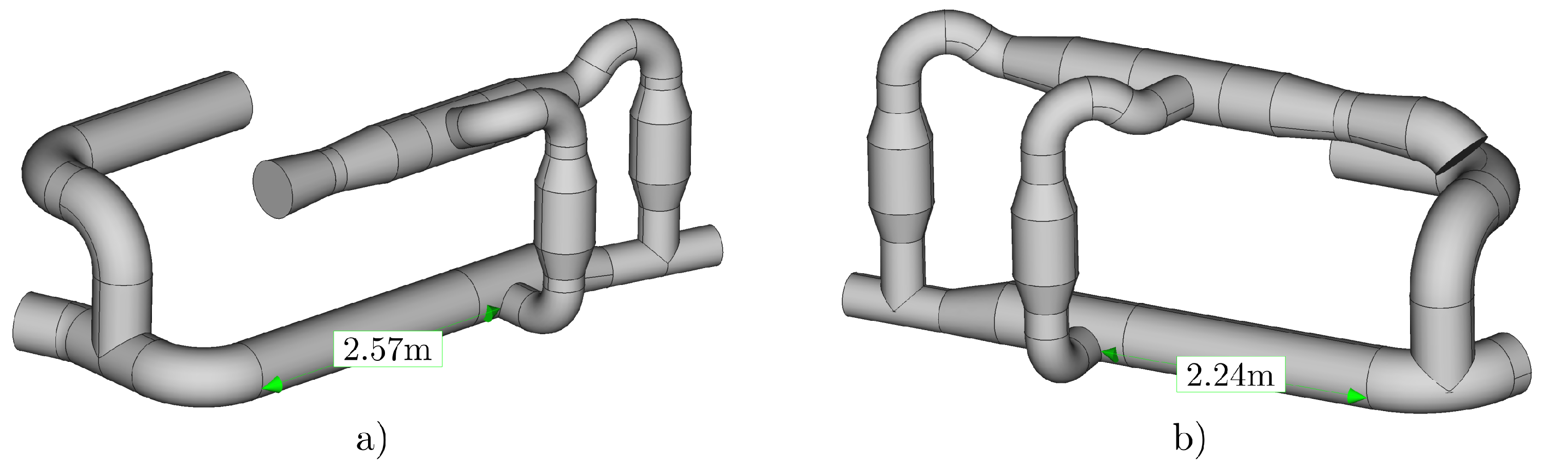
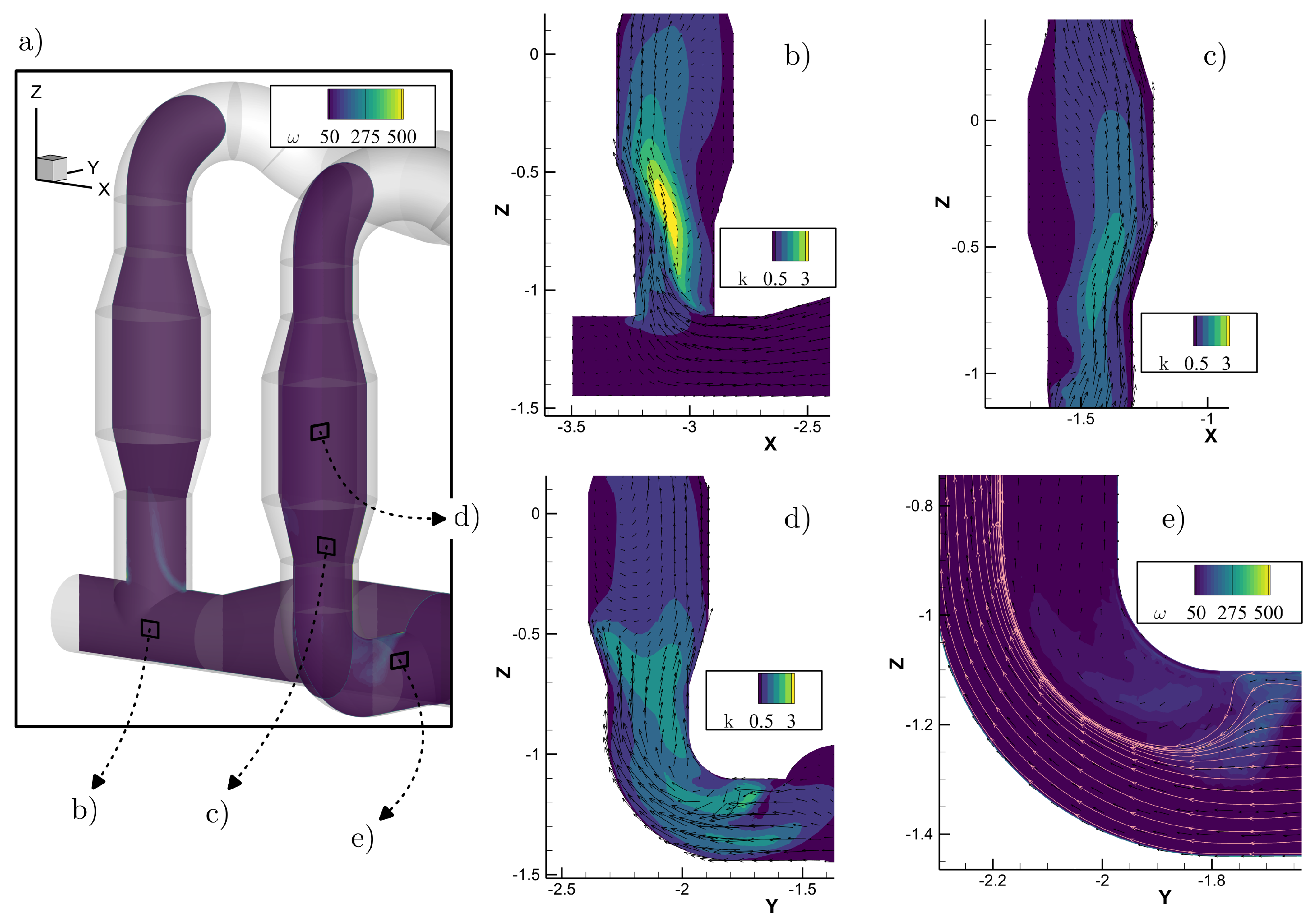
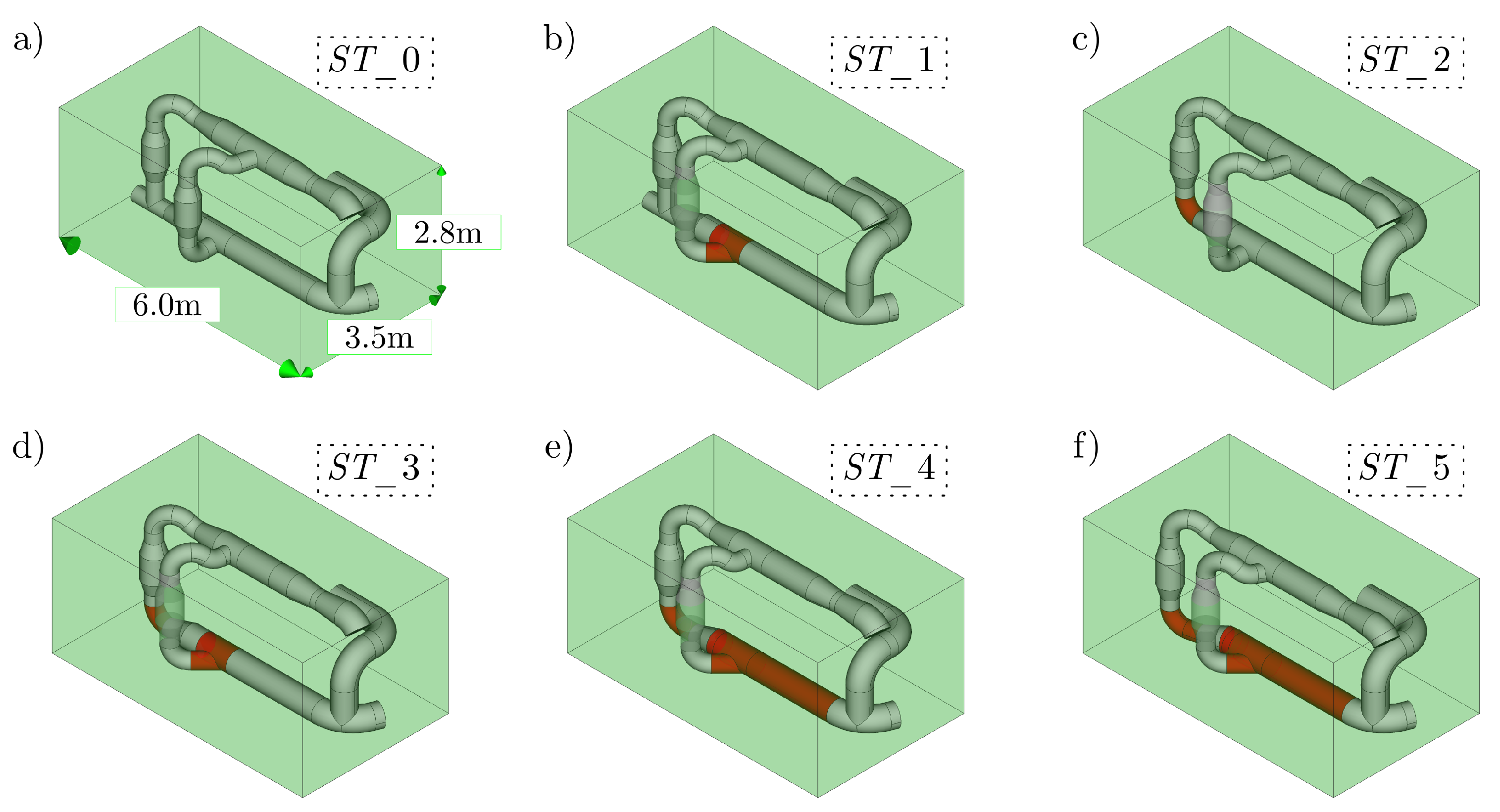
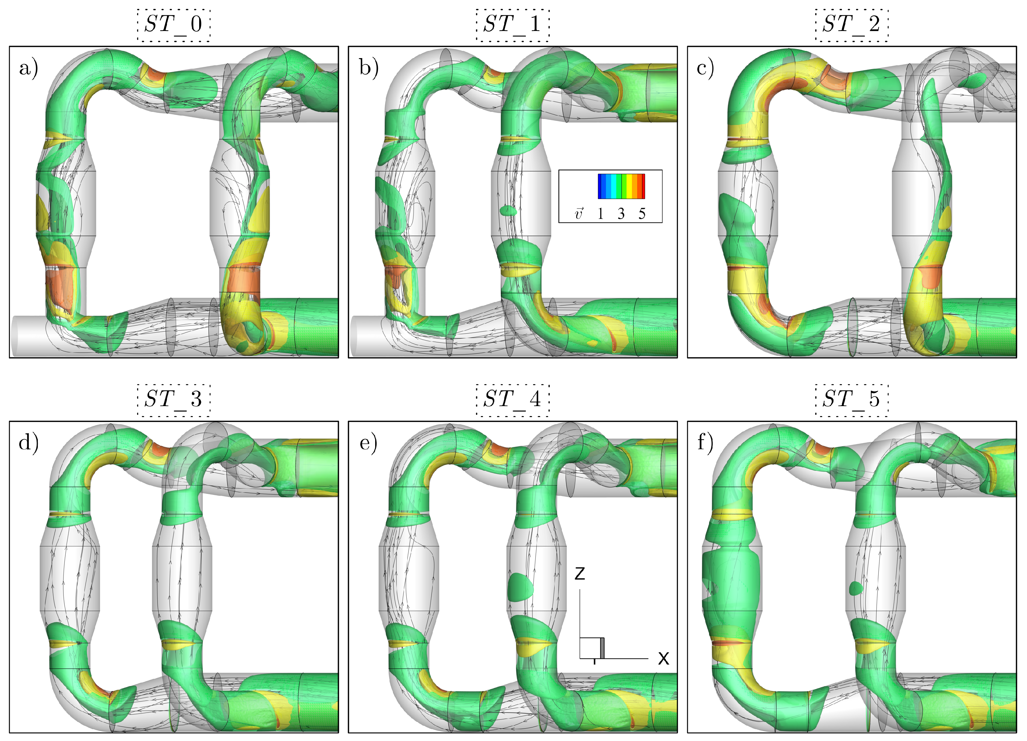
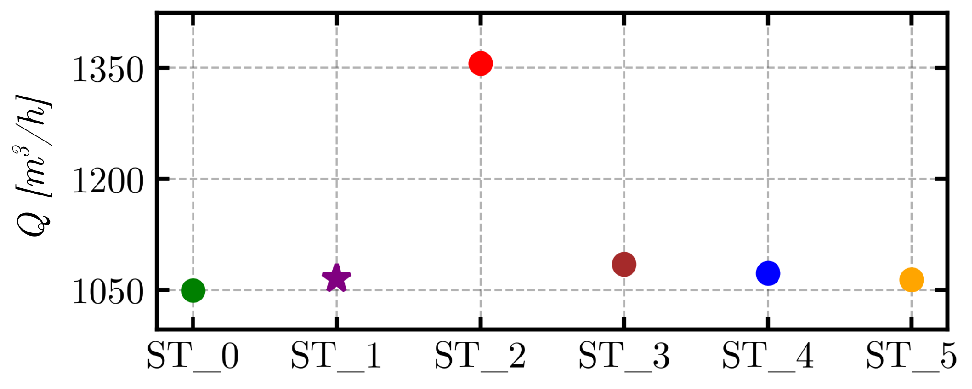
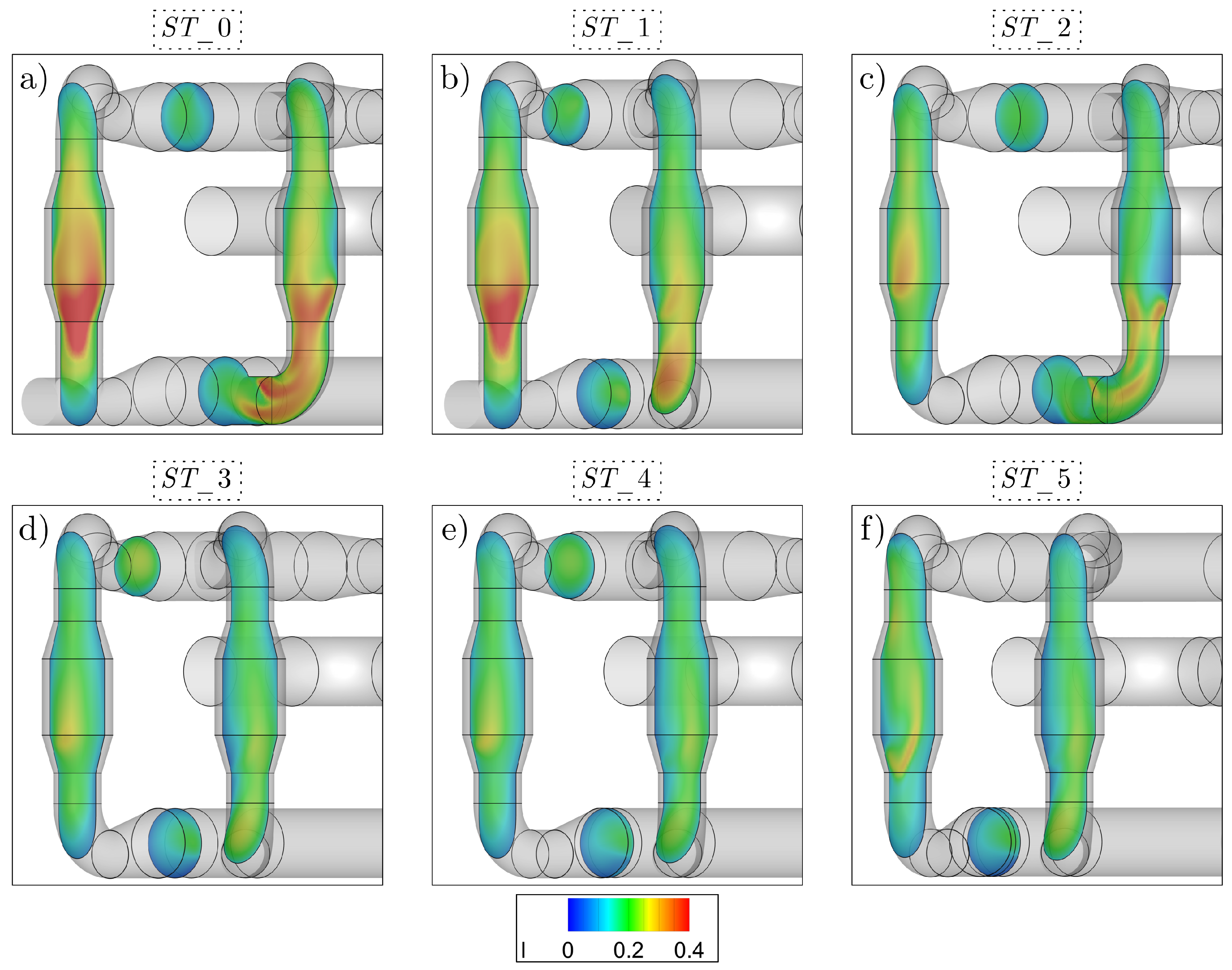
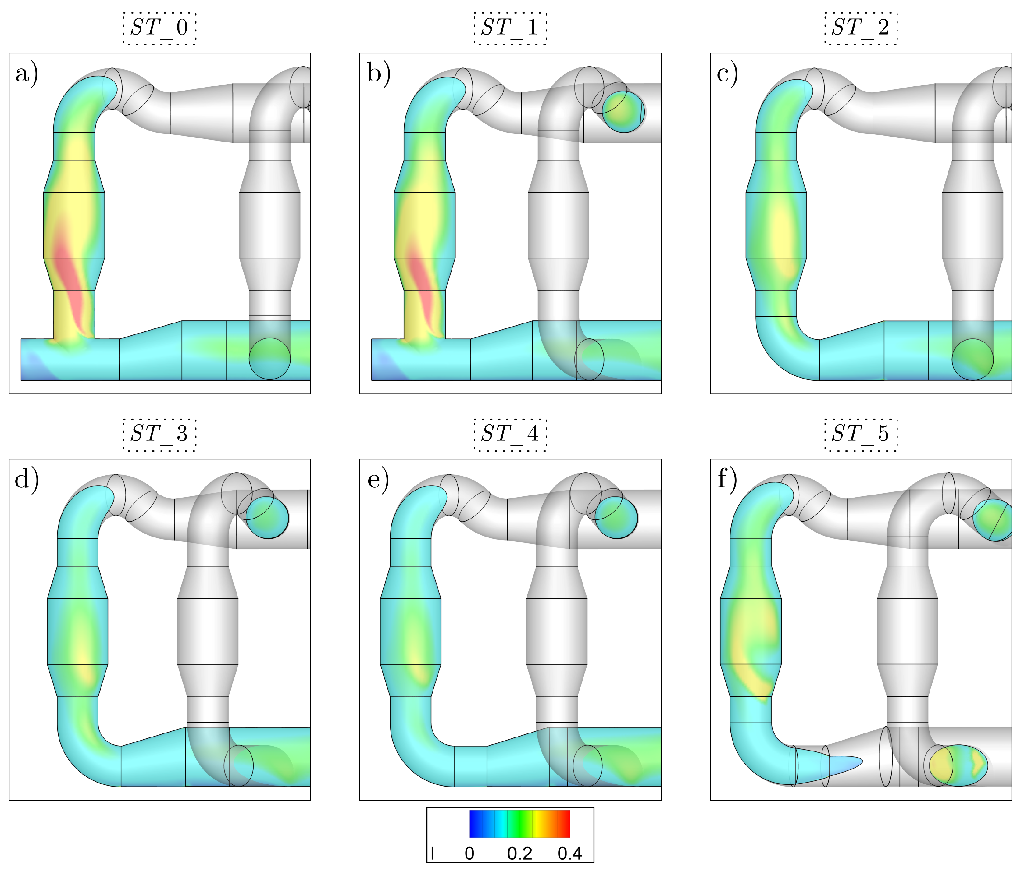
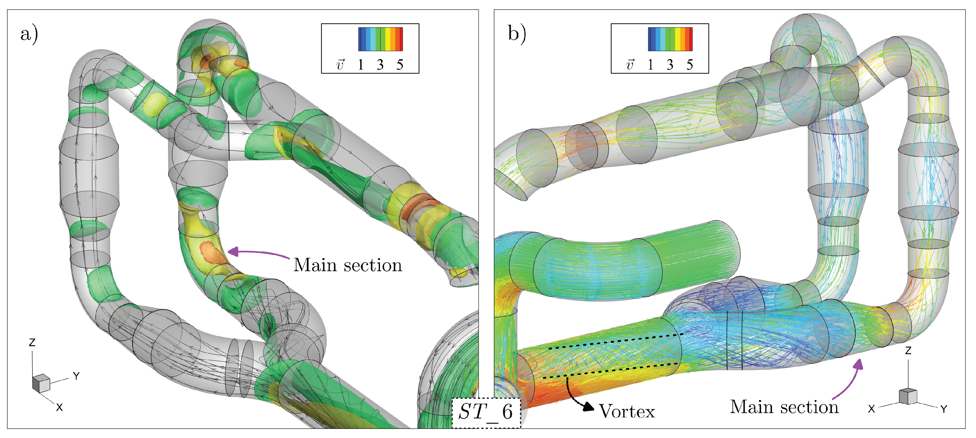
3.2. Analysis of Possible Pipeline Geometry Changes

As discussed throughout this article, the already-built pipeline systems in the newbuilding’s engine room were analyzed to ensure compliance with the manufacturer’s requirements. Based on the detailed fluid flow analysis, several conclusions were drawn that can guide upgrades to the current geometry. The objectives are to propose modifications to the existing pipeline layout, evaluate their impact on fluid flow, and highlight key considerations for designing pipeline systems that enhance flow uniformity and minimize potential damage to UV lamps inside the UVRs. To this end, five alternative pipeline layouts for the starboard engine room were developed, as illustrated in Figure 13.

Figure 13a illustrates the current pipeline layout on the starboard side. The green cuboid represents the engine room space, serving as a boundary for designing alternative layouts. The filter attached to the pipeline inlet (see Figure 2) maintains sufficient clearance from other pipes to ensure the ease of assembly and disassembly, while the UVRs are spaced appropriately. Figure 13b–f highlight the variations in the pipeline layouts, marked in red, with a focus on regions before the UVRs. In Figure 13b (ST_1), the side pipeline section is angled 45° less than the original layout’s 90°. Figure 13c (ST_2) replaces the T-junction in the main pipeline with an elbow featuring a diameter of 355.6 mm, a thickness of 8 mm, and a curvature radius of 356 mm, bringing the main pipeline UVR closer to the inlet. Figure 13d (ST_3) combines the modifications from ST_1 and ST_2. In Figure 13e (ST_4), an additional straight pipe segment is introduced between the pipe reduction and elbow in the main pipe section, while the side pipe section is slightly shifted closer to the filter. Finally, Figure 13f (ST_5) adopts a layout similar to the port-side configuration, directing the main pipe section 13° to the left (top view) compared to ST_4.

Following the development of the new pipeline layouts within the engine room boundaries, a fluid flow analysis was conducted. To visualize seawater propagation, the coarse streamlines and translucent pipeline layouts around the UVRs are presented in Figure 14, which also includes the velocity magnitude iso-surfaces.

The velocity magnitude legend and view are consistent across all subfigures. The iso-surfaces are highlighted for velocity values of 3, 4, and 5 m/s. The pipeline layout consists of two pipe diameters: 355.6 mm and 508 mm, as detailed in Section 2.1. For the larger pipes, a velocity magnitude of approximately 3 m/s corresponds to a volume flow rate of 2000 ${\mathrm{m}}^3/\mathrm{h}$. The desired flow rate for the UVRs is half the nominal Q (2000 ${\mathrm{m}}^3/\mathrm{h}$), meaning that no iso-surfaces should be visible inside the UVRs, as this would indicate velocities at least twice the desired value. Consequently, it is essential to evaluate the overall volume flow rate at the UVR inlets and assess fluid flow uniformity before seawater enters the UVRs.

The current pipeline layout on the starboard-side BWTU was previously analyzed and is shown again in Figure 14a from a different visualization perspective. The highest velocities are observed in both the main and side sections just before the UVR inlets due to sharp 90° bends in both sections, as discussed in detail in Section 3.1. To address this issue, modifications were made to reduce the velocity magnitudes in the pipe segments before the UVR inlets. By adjusting the side pipeline section’s connection to the main pipeline to form a 45° angle, the velocity magnitudes are reduced (Figure 14b). This adjustment also redistributes the volume flow rate, directing more seawater through the side pipe section, as illustrated in Figure 15.

In the case of ST_2, shown in Figure 14c, replacing the T-junction with an elbow slightly improves the UVR’s flow uniformity, as streamlines are more evenly distributed across the UVR. However, the velocity reduction is minimal, and the side pipe section shows fewer streamlines within the UVR, making it appear relatively empty. This is attributed to a poor seawater distribution between the parallel UVRs, with a relative error exceeding 35% compared to the ideal Q of 1000 ${\mathrm{m}}^3/\mathrm{h}$. Comparing ST_2 with ST_0 reveals that the slight improvement in seawater uniformity does not justify the worsened distribution between the UVRs. However, comparing ST_1 with ST_0 demonstrates better uniformity but a slightly worse Q distribution. To address these issues, a combination of ST_1 and ST_2 was analyzed (Figure 14d). This layout significantly improves seawater uniformity, with nearly flat streamlines throughout the UVR, no visible iso-surfaces, and reduced velocities before the UVR inlets. However, the Q distribution worsens slightly. Despite this drawback, the improved seawater uniformity supports the use of this layout. To further optimize performance, ST_4 was introduced (Figure 14e), bringing the side pipe section closer to the inlet. This layout achieves similar results to ST_3 but with slightly reduced velocity magnitudes in the main pipeline elbow and slightly higher values in the side pipe section UVR. These improvements result from a better Q distribution between the UVRs. Finally, ST_5 (Figure 14f) achieves a slight improvement in the Q distribution but introduces a small elbow that redirects the flow after the side section. This modification negatively impacts the seawater uniformity in the main pipe section, ultimately failing to justify the use of this layout.

Building upon the preceding analysis, the turbulence intensity is quantified in Figure 16 and Figure 17. These figures depict two-dimensional sections, in contrast to the three-dimensional iso-surfaces presented earlier. Both figures use the same contour levels and legend. Specifically, Figure 16 displays a section cut in the ZY-plane, while Figure 17 shows a section cut in the ZX-plane.

The T-junction in the main pipe section causes the most significant disruption to flow uniformity, as shown in Figure 16a,b, as well as in Figure 17a,b from a different section cut. Similarly, the T-junction in the side pipe section contributes to a higher turbulence intensity, evident in Figure 16c. By modifying these critical locations, turbulence reduction is achieved, as illustrated in Figure 16d,e and Figure 17d,e for cases ST_3 and ST_4. The greatest improvement results from introducing an elbow instead of a T-junction. Moreover, bending the T-junction in the side pipe section noticeably reduces the overall turbulence intensity. However, as previously noted, bending the pipeline before the main pipe UVR in case ST_5 negatively impacts the turbulence intensity compared to in cases ST_3 and ST_4.

Overall, layout changes such as ST_3 and ST_4 improve fluid flow uniformity without significantly compromising the Q distribution between the UVRs, with relative errors of 8.49% and 7.27%, respectively. These results demonstrate how small geometry adjustments can have a substantial impact on performance. Even in a constrained engine room with limited opportunities for major pipeline modifications, meaningful improvements can be achieved.

In contrast, more extensive layout changes are presented in Figure 18 while maintaining the fixed initial section near the filter and adhering to the defined boundaries of the engine room’s free space. The goal was to create two symmetrical sections up to the UVR outlet, where the side section reconnects with the main pipeline, which retains the same alignment as in ST_0.

The initial assumption for a symmetrical layout is that the volume flow rate should be equal for both sections. However, this is not the case here, as Q is higher in the main pipe section, with a relative error of 14.57% compared to an ideal Q of 1000 ${\mathrm{m}}^3/\mathrm{h}$. Figure 19a, using the same visualization techniques as Figure 14, highlights the velocity magnitude differences between the main and side pipe sections. Higher velocities are evident in the main pipe section, caused by the greater volume of seawater flowing through that section.

At first glance, it seems unusual that two symmetrical sections exhibit such significant variations in the volume flow rate. The explanation can be found in Figure 19b, which highlights a vortex in the long straight pipe. Despite the two parallel, symmetrical sections built after the straight pipe, seawater is not distributed equally. The reason lies in the pipeline section before the straight pipe, consisting of several bends and a large T-junction with a curved lower pipe. As a result, a strong vortex forms, visualized in Figure 19b, produced by the sharp and curved T-junction where the fluid flow arrives with slightly energized vortices from the elbow bending. This vortex in the long straight pipe pushes seawater through the main section and prevents the higher velocity flow at the bottom of the pipe from overcoming the vortex and distributing it more evenly.

Overall, even with such symmetrical sections, there is no guarantee of an equal and uniform fluid flow distribution due to the influence of upstream sections. To optimize this symmetrical design, the long straight pipe should be extended to allow for fluid flow stabilization, or the initial part of the starboard pipeline layout should be modified. As discussed previously, the engine room space often dictates design choices, but improvements are possible, even in confined spaces, as demonstrated by the other layouts presented earlier.

4. Conclusions

A CFD investigation of ballast water treatment units (BWTUs) installed in a newbuilding self-discharging bulk carrier’s engine room was conducted to assess the fluid flow uniformity and volume flow rate (Q) through the UV reactors. The study focused on the seawater flow before the UVR entrance and the correlation of the volume flow rates between two parallel UVRs. Simulations were performed for both starboard- and port-side layouts with nominal volume flow rates of 1000, 1900, and 2000 ${\mathrm{m}}^3/\mathrm{h}$. Numerical verification of the simulations included mesh quality metrics, boundary layer analysis, mesh sensitivity studies, and residual monitoring.

The current pipeline layouts showed relative errors of 4.95% for the starboard side and 2.35% for the port side at a nominal flow rate of 2000 ${\mathrm{m}}^3/\mathrm{h}$, exceeding the manufacturer’s recommended limit of 1000 ${\mathrm{m}}^3/\mathrm{h}$ per UV reactor. A 5% reduction in the initial flow rate ensured compliance with the recommended threshold for all UV reactors. Nevertheless, a Q analysis should be complemented with a uniformity assessment, which revealed high velocities before and through the UVRs with an uneven distribution. To address these issues, six additional simulations with layout modifications were conducted to identify each design’s strengths and weaknesses. ST_3 and ST_4 demonstrated the best results when considering both the volume flow rate distribution and fluid flow uniformity. These modifications showed significant improvements in fluid flow uniformity compared to the original ST_0 case. However, they also resulted in a small increase in the relative error of the Q distribution in the main pipe section of the ST_3 and ST_4 layouts, with values of 8.49% and 7.27%, respectively.

BWTU systems are crucial for marine environmental protection and global ecological balance. This research contributes to the field by bridging the gap between scientific analysis and practical implementation on ships. A detailed CFD analysis of real-world scenarios can significantly impact the modeling and upgrading of pipeline layouts for implementation in ship engine rooms. By optimizing pipeline layouts, BWTU efficiency can be improved, leading to a reduced bacterial presence, enhanced equipment safety, and potential financial savings. While turbulence is inevitable in certain parts of pipeline systems, a strategic approach can minimize its impact. This study demonstrates the potential of CFD analysis to optimize BWTU systems, paving the way for more efficient and environmentally friendly maritime operations.

References

1. Rebeca, G. Review of Maritime Transport; United Nations: Geneva, Switzerland, 2024. [Google Scholar]
2. EMSA—European Maritime Safety Agency. Ballast Water Management—Guidance for Best Practices on Sampling; EMSA—European Maritime Safety Agency: Lisboa, Portugal, 2019.
3. Chan, F.T.; Macisaac, H.J.; Bailey, S.A. Relative importance of vessel hull fouling and ballast water as transport vectors of nonindigenous species to the canadian arctic. Can. J. Fish. Aquat. Sci. 2015, 72, 1230–1242. [Google Scholar] [CrossRef]
4. Coutts, A.D.; Dodgshun, T.J. The nature and extent of organisms in vessel sea-chests: A protected mechanism for marine bioinvasions. Mar. Pollut. Bull. 2007, 54, 875–886. [Google Scholar] [CrossRef] [PubMed]
5. Argüello, G.; Krabbe, N.; Langlet, D.; Hassellöv, I.M.; Martinson, C.; Helmstad, A. Regulation of ships at anchor: Safety and environmental implications. Mar. Policy 2022, 140, 105052. [Google Scholar] [CrossRef]
6. Watson, S.J.; Ribó, M.; Seabrook, S.; Strachan, L.J.; Hale, R.; Lamarche, G. The footprint of ship anchoring on the seafloor. Sci. Rep. 2022, 12, 7500. [Google Scholar] [CrossRef]
7. Minchin, D. Aquaculture and transport in a changing environment: Overlap and links in the spread of alien biota. Mar. Pollut. Bull. 2007, 55, 302–313. [Google Scholar] [CrossRef]
8. Molnar, J.L.; Gamboa, R.L.; Revenga, C.; Spalding, M.D. Assessing the global threat of invasive species to marine biodiversity. Front. Ecol. Environ. 2008, 6, 485–492. [Google Scholar] [CrossRef]
9. Vilà, M.; Basnou, C.; Pyšek, P.; Josefsson, M.; Genovesi, P.; Gollasch, S.; Nentwig, W.; Olenin, S.; Roques, A.; Roy, D.; et al. How well do we understand the impacts of alien species on ecosystem services? A pan-European, cross-taxa assessment. Front. Ecol. Environ. 2010, 8, 135–144. [Google Scholar] [CrossRef]
10. David, M.; Gollasch, S.; Pavliha, M. Global ballast water management and the “same location” concept: A clear term or a clear issue? Ecol. Appl. 2013, 23, 331–338. [Google Scholar] [CrossRef]
11. Strayer, D.L. Alien species in fresh waters: Ecological effects, interactions with other stressors, and prospects for the future. Freshw. Biol. 2010, 55, 152–174. [Google Scholar] [CrossRef]
12. Baek, J.T.; Hong, J.H.; Tayyab, M.; Kim, D.W.; Jeon, P.R.; Lee, C.H. Continuous bubble reactor using carbon dioxide and its mixtures for ballast water treatment. Water Res. 2019, 154, 316–326. [Google Scholar] [CrossRef]
13. Lakshmi, E.; Priya, M.; Achari, V.S. An overview on the treatment of ballast water in ships. Ocean Coast. Manag. 2021, 199, 105296. [Google Scholar] [CrossRef]
14. Drillet, G.; Gianoli, C.; Gang, L.; Zacharopoulou, A.; Schneider, G.; Stehouwer, P.; Bonamin, V.; Goldring, R.; Drake, L.A. Improvement in compliance of ships’ ballast water discharges during commissioning tests. Mar. Pollut. Bull. 2023, 191, 114911. [Google Scholar] [CrossRef] [PubMed]
15. International Maritime Organization. International Convention for the Control and Management of Ships’ Ballast Water and Sediments; Convention BWM/CONF/36; International Maritime Organization: London, UK, 2004. [Google Scholar]
16. International Maritime Organization. Guidelines for Approval of Ballast Water Management Systems (G8); Resolution MEPC.174(58); International Maritime Organization: London, UK, 2008. [Google Scholar]
17. International Maritime Organization. Procedure for Approval of Ballast Water Management Systems That Make Use of Active Substances (G9); Resolution MEPC.169(57); International Maritime Organization: London, UK, 2008. [Google Scholar]
18. Campara, L.; Francic, V.; Maglic, L.; Hasanspahic, N. Overview and Comparison of the IMO and the US Maritime Administration Ballast Water Management Regulations. J. Mar. Sci. Eng. 2019, 7, 283. [Google Scholar] [CrossRef]
19. Tsolaki, E.; Diamadopoulos, E. Technologies for ballast water treatment: A review. J. Chem. Technol. Biotechnol. 2010, 85, 19–32. [Google Scholar] [CrossRef]
20. Werschkun, B.; Sommer, Y.; Banerji, S. Disinfection by-products in ballast water treatment: An evaluation of regulatory data. Water Res. 2012, 46, 4884–4901. [Google Scholar] [CrossRef]
21. Balaji, R.; Yaakob, O.; Koh, K.K. A review of developments in ballast water management. Environ. Rev. 2014, 22, 298–310. [Google Scholar] [CrossRef]
22. Werschkun, B.; Banerji, S.; Basurko, O.C.; David, M.; Fuhr, F.; Gollasch, S.; Grummt, T.; Haarich, M.; Jha, A.N.; Kacan, S.; et al. Emerging risks from ballast water treatment: The run-up to the International Ballast Water Management Convention. Chemosphere 2014, 112, 256–266. [Google Scholar] [CrossRef]
23. Bakalar, G. Comparisons of interdisciplinary ballast water treatment systems and operational experiences from ships. SpringerPlus 2016, 5, 1–12. [Google Scholar] [CrossRef]
24. Vorkapić, A.; Radonja, R.; Zec, D. Cost efficiency of ballast water treatment systems based on ultraviolet irradiation and electrochlorination. Promet-Traffic Transp. 2018, 30, 343–348. [Google Scholar] [CrossRef]
25. Sayinli, B.; Dong, Y.; Park, Y.; Bhatnagar, A.; Sillanpää, M. Recent progress and challenges facing ballast water treatment—A review. Chemosphere 2022, 291, 132776. [Google Scholar] [CrossRef]
26. Stehouwer, P.P.; Buma, A.; Peperzak, L. A comparison of six different ballast water treatment systems based on UV radiation, electrochlorination and chlorine dioxide. Environ. Technol. 2015, 36, 2094–2104. [Google Scholar] [CrossRef] [PubMed]
27. Petersen, N.B.; Madsen, T.; Glaring, M.A.; Dobbs, F.C.; Jørgensen, N.O. Ballast water treatment and bacteria: Analysis of bacterial activity and diversity after treatment of simulated ballast water by electrochlorination and UV exposure. Sci. Total Environ. 2019, 648, 408–421. [Google Scholar] [CrossRef] [PubMed]
28. Pećarević, M.; Mikuš, J.; Prusina, I.; Juretić, H.; Cetinić, A.B.; Brailo, M. New role of hydrocyclone in ballast water treatment. J. Clean. Prod. 2018, 188, 339–346. [Google Scholar] [CrossRef]
29. Lundgreen, K.; Holbech, H.; Pedersen, K.L.; Petersen, G.I.; Andreasen, R.R.; George, C.; Drillet, G.; Andersen, M. UV fluences required for compliance with ballast water discharge standards using two approved methods for algal viability assessment. Mar. Pollut. Bull. 2018, 135, 1090–1100. [Google Scholar] [CrossRef]
30. Romero-Martínez, L.; van Slooten, C.; van Harten, M.; Nebot, E.; Peperzak, L. Comparative assessment of four ballast water compliance monitoring devices with natural UV-treated water using IMO’s monitoring approaches. Mar. Pollut. Bull. 2024, 209, 117193. [Google Scholar] [CrossRef]
31. Thach, N.D.; Hung, P.V. Development of UV reactor controller in ballast water treatment system to minimize the biological threat on marine environment. J. Sea Res. 2024, 198, 102465. [Google Scholar] [CrossRef]
32. Joo, J.; Jung, G.; Oh, I.; Rhee, T. Validation test on real scale uv reactor for ballast water treatment. Environ. Eng. Res. 2021, 26, 190455. [Google Scholar] [CrossRef]
33. Zhang, N.; Hu, K.; Shan, B. Ballast water treatment using UV/TiO2 advanced oxidation processes: An approach to invasive species prevention. Chem. Eng. J. 2014, 243, 7–13. [Google Scholar] [CrossRef]
Figure 1. BWTU arrangement on ship’s engine room port side.
Jmse 13 00743 g001
Figure 2. BWTU arrangement on ship’s engine room starboard side.
Jmse 13 00743 g002
Figure 3. The 3D CAD models of (a) port-side and (b) starboard-side BWTUs. Blue and red arrows indicate inlet and outlet flows, respectively.
Jmse 13 00743 g003
Figure 4. Flow direction in main and side pipe sections with emphasized critical UVR inlets at starboard side.
Jmse 13 00743 g004
Figure 5. Wall y + distribution for (ac) port-side BWTU at volume flow rates of 1000, 1900, and 2000 m 3 / h and (df) starboard-side BWTU at corresponding flow rates.
Jmse 13 00743 g005
Figure 6. (a) Grid sensitivity analysis at the UV reactor inlet for the port-side layout; (b) distribution of different cell types in straight pipe sections and the T-junction for the medium mesh case.
Jmse 13 00743 g006
Figure 7. Residual convergence for (ac) starboard-side BWTU at volume flow rates of 1000, 1900, and 2000 m 3 / h and (df) port-side BWTU at corresponding flow rates.
Jmse 13 00743 g007
Figure 8. Streamline visualization of velocity magnitude in m/s for the port-side pipeline system at volume flow rates of (a) 1000 m 3 / h , (b) 1900 m 3 / h , and (c) 2000 m 3 / h .
Jmse 13 00743 g008
Figure 9. Surface integral values of the volume flow rate (Q) at the UVR inlets over iterations for the (a) main pipe and (b) side pipe at an initial Q of 2000 m 3 / h .
Jmse 13 00743 g009
Figure 10. Streamline visualization at 2000 m 3 / h for the starboard pipeline with a consistent velocity color bar: (a) full pipeline layout; (b,c) front and back views of UVRs.
Jmse 13 00743 g010
Figure 11. Emphasized distance between the start of the straight pipe and the beginning of the side pipe section for (a) port-side layout and (b) starboard-side layout.
Jmse 13 00743 g011
Figure 12. Visualization of vorticity ( ω ) (a,e) and turbulent kinetic energy (k) (bd) in the starboard-side pipeline system.
Jmse 13 00743 g012
Figure 13. Starboard BWTU pipeline layouts: (a) current design (ST_0); (bf) modifications (ST_1–ST_5) with changes in red.
Jmse 13 00743 g013
Figure 14. Velocity magnitude iso-surfaces (3, 4, and 5 m/s) and streamlines for starboard pipeline: (a) ST_0 (current layout), (b) ST_1 (45° side pipe connection), (c) ST_2 (elbow replacing T-junction), (d) ST_3 (combination of ST_1 and ST_2), (e) ST_4 (side pipe section closer to the inlet), and (f) ST_5 (small elbow after side pipe section).
Jmse 13 00743 g014
Figure 15. Volume flow rates at UVR inlets for ST_0 (current layout) and ST_1 – ST_5 (modified layouts). Circular markers indicate main pipe dominance; star markers indicate side pipe dominance.
Jmse 13 00743 g015
Figure 16. Turbulence intensity contours in the ZY-plane for six pipeline layouts.
Jmse 13 00743 g016
Figure 17. Turbulence intensity contours in the ZX-plane for six pipeline layouts.
Jmse 13 00743 g017
Figure 18. Proposed symmetrical pipeline layout (ST_6) for the starboard BWTU, with engine room boundaries shown as a green cuboid.
Jmse 13 00743 g018
Figure 19. Velocity iso-surfaces and streamlines for ST_6: (a) higher velocities in the main section and (b) vortex formation in the straight pipe affecting flow distribution.
Jmse 13 00743 g019