Parameterizing the Tip Effects of Submerged Vegetation in a VARANS Solver

Abstract

This paper presents an experimental and numerical investigation of submerged vegetation flow, with a particular focus on vegetation-related terms, especially in the vicinity of the free end. Experimental results indicate that substantial shear stress is observed near the top of vegetation, where the drag coefficient increases significantly due to the disturbance caused by the free end. Furthermore, wake generation is notably suppressed, particularly at heights where wake-generated turbulence dominates, leading to a reduction in turbulent kinetic energy (TKE). A numerical model based on the volume-averaged Reynolds-averaged Navier–Stokes (VARANS) equations was developed, incorporating a vertically varying drag coefficient. The two-scale $⟨k⟩-⟨\epsilon ⟩$ turbulence model is further modified with the inclusion of a new damping function to capture the suppression of wake generation. The model accurately simulates both unidirectional and oscillatory flows, as well as the associated turbulence structures, with good agreement with experimental measurements. The influence of the tips on wave-induced currents, mass transport and TKE distribution is also investigated. It was found that the tip effects play a significant role in strengthening wave-induced currents at the top of loosely arranged, short, and sparse vegetation, with shear kinetic energy (SKE) serving as a critical component of TKE, contributing to the nonuniform distribution. Both Eulerian currents and Stokes drift contribute to streaming in the direction of wave propagation near the vegetation top, which intensifies with increasing solid volume fraction, while tip effects further enhance the onshore mass transport. Within the vegetation, mass transport is more sensitive to wave period and wave height, shifting from onshore to offshore as wavelength increases under constant water depth.

1. Introduction

Aquatic vegetation plays a crucial role in coastal ecosystems by influencing both biological and hydrodynamic processes. It provides natural protection against storm surges, serves as a habitat for marine organisms, and enhances biodiversity in wetland ecosystems [1]. The high permeability of vegetation improves water circulation, nutrient retention, and water quality, while also acting as a significant carbon sink [2]. Coastal ecosystems such as tidal marshes, mangroves, sandbars, coral reefs, and shellfish reefs achieve these functions by generating drag forces and altering hydrodynamic processes [3,4]. Aquatic vegetation buffers wave action, promotes wave breaking, and enhances wave energy dissipation [5,6,7,8]. By reducing flow velocity, it facilitates sediment deposition and minimizes sediment resuspension within the vegetation zone [9,10,11,12], offering a natural solution to sea-level rise. The steady flow within vegetation zones enhances nutrient exchange and seed dispersal, promoting vegetation expansion [13,14].

The interaction between flow and vegetation has been studied and recognized as a key source of resistance and turbulence within vegetated regions. Research on emergent vegetation has provided insights relevant to submerged vegetation, revealing that the drag coefficient decreases with increasing vegetation density due to eddy–eddy and eddy–stem interactions, as well as the blocking effect on local flow [15,16]. Additionally, intense small-scale turbulence generated in the wake of vegetation stems enhances mixing, nutrient exchange, and sediment resuspension [9,10,17]. Based on the balance between wake production and viscous dissipation, Nepf [18] and Tanino and Nepf [19] proposed a model for wake-scale turbulence as follows

$$〈k〉=\gamma {\left[C_d{\displaystyle \frac{2\varphi }{\left(1-\varphi \right)\pi }}\right]}^{2/3}{〈u〉}^2$$

(1)

where $\gamma$ is an empirical constant, $\varphi ={\displaystyle \frac{\pi }{4}}a{b}_v$ represents the volume fraction occupied by vegetation, and $a$ and $b_v$ denote the frontal area density and vegetation diameter, respectively.

Recently, there have been extensive experimental and numerical studies on submerged vegetation [20,21,22,23,24,25]. Ghisalberti and Nepf [26] conducted laboratory experiments demonstrating that the development of a shear layer near the vegetation top results from discontinuity in drag. Both shear-scale and wake-scale turbulence dynamics contribute to vertical exchange between the vegetation and the overlying water [17,27,28]. To estimate vegetation-induced flow resistance, Shimizu and Tsujimoto [29] and López and García [30] introduced vegetation-related terms as source terms in both the momentum and turbulence equations to represent the effects of submerged vegetation. King et al. [20] extended this model by incorporating an additional WKE equation to account for turbulence at the vegetation diameter scale. However, O’Donncha et al. [31] highlighted that the application of the model is constrained by the lack of a detailed parameterization of the drag coefficient for submerged vegetation. Xuan et al. [32] further emphasized the importance of accurately resolving the spatial distribution of drag forces when modeling flow velocities within the vegetation.

Numerous studies have investigated the distribution of drag coefficients [26,31,33,34,35,36]. Although the identified peak locations vary among these studies, the overall distribution patterns exhibit notable similarity. Specifically, elevated drag coefficients near vegetation tips are attributed to reduced wake pressure induced by tip vortices, gradually decreasing to a near-constant value further into the interior of submerged vegetation. This trend closely resembles that observed for a single cylinder, where tip effects similarly influence drag distribution [37]. The free end of a single cylinder significantly alters flow structures, impacting spanwise pressure distribution, vortex formation, and vortex-shedding patterns. A similar vortex-shedding mechanism has also been observed in vegetated flows. According to the two-dimensional DNS study by Nicolle and Eames [16], interactions between stem wakes remain weak at vegetation densities up to 5%, closely resembling the wake patterns observed behind a single cylinder. Similarly, experimental results from Tang et al. [38] indicate that, at a vegetation density of 2.54%, the velocity field and turbulence characteristics near the vegetation exhibit strong similarities to those of a single-cylinder wake. This observation inspires the consideration of single-cylinder tip effects within vegetated flows. Most existing studies characterize the drag coefficient distribution based on the relative vegetation height as a characteristic length scale, while neglecting the characteristic scale associated with tip vortices generated by the free ends. Moreover, volume-averaged coastal wave models [14,21,22] often incorporate depth-averaged vegetation-related terms, which can yield satisfactory predictions of wave energy dissipation. However, this approach inherently neglects the vertical variability in vegetation-induced flow resistance and thus proves inadequate for resolving detailed flow structures within the vegetation. To date, the role of tip effects in modulating vegetation-flow interactions under wave forcing remains insufficiently understood. This study aims to develop a generalized parameterization approach for submerged vegetation, explicitly accounting for tip effects on vegetation-related terms. A new model was formulated based on the VARANS equations and a modified two-scale $〈k〉-〈\epsilon 〉$ framework from King et al. [20], incorporating tip effects. A series of submerged vegetation experiments were conducted to systematically examine the influence of tip effects on vegetation-related parameters, including drag force and wake production. The model was further validated against a broad range of published data for unidirectional and oscillatory flow conditions, encompassing porosities ranging from 0.97% to 7.94%. Additionally, the impact of tip effects on flow structures, mass transport and TKE budgets is analyzed, with the conclusions summarized in Section 6.

2. Numerical Model

2.1. Hydrodynamic Model

In turbulent flow, all flow variables, represented by $\phi$, are decomposed into a time-averaged component $\overline{\phi }$ and a turbulent fluctuation component ${\phi }^{\prime }$, along with the ensemble-intrinsic volume average ${〈\overline{\phi }〉}^f$. The mean flow field is governed by the following VARANS equations

$${\displaystyle \frac{\partial 〈\overline{u_i}〉}{\partial x_i}}=0$$

(2)

$${\displaystyle \frac{1}{n}}{\displaystyle \frac{\partial 〈\overline{u_i}〉}{\partial t}}+{\displaystyle \frac{〈\overline{u_j}〉}{n}}{\displaystyle \frac{\partial }{\partial x_j}}{\displaystyle \frac{〈\overline{u_i}〉}{n}}=-{\displaystyle \frac{1}{\rho }}{\displaystyle \frac{\partial {〈\overline{p}〉}^f}{\partial x_i}}+{\displaystyle \frac{1}{n}}{\displaystyle \frac{\partial 〈\overline{{\tau }_{ij}}〉}{\partial x_j}}+g_i-f_i$$

(3)

where $u_i$ is the flow velocity (simplified as $u_i=(u,v)$); $x_i$ denotes the Cartesian coordinate; $t$ is time, ${\rho }_f$ is the density of the fluid; $p$ is pressure; ${\tau }_{ij}$ is the viscous stress tensor of the mean flow; $g_i$ is the $i$th component of the gravitational acceleration; $n=1-\varphi$ is the porosity of the vegetation region; “〈 〉” and “〈 〉^f” refer to the Darcy’s volume averaging operator and intrinsic averaging operator, respectively.

In the VARANS model, the force term $f_i=f_{di}+f_{Ii}$ consists of vegetation-induced drag and inertial force. For straight vegetation, the vertical force is negligible compared to other components. Thus, only horizontal force was considered in this model. Incorporating porosity effects, the total force could be simulated as follows

$$f_i={\displaystyle \frac{1}{2}}{\displaystyle \frac{C_{d}a}{n^3}}\left|〈u〉\right|〈u〉+C_M{\displaystyle \frac{1-n}{n^2}}{\displaystyle \frac{\partial 〈u〉}{\partial t}}$$

(4)

The shear stress $〈\overline{{\tau }_{ij}}〉$ is the sum of viscous stress, Reynolds stress, $-〈\overline{u_i^{\prime }{u}_j^{\prime }}〉$, and dispersive stress, $-〈{\overline{u_i}}^{″}{\overline{u_j}}^{″}〉$, which is generated by the spatial heterogeneity of the time-averaged velocity within the vegetation.

$$〈\overline{{\tau }_{ij}}〉=-〈\overline{u_i^{\prime }{u}_j^{\prime }}〉-〈{\overline{u_i}}^{″}{\overline{u_j}}^{″}〉+\upsilon {\displaystyle \frac{\partial 〈\overline{u_i}〉}{\partial x_j}}$$

(5)

For a wide range of vegetation densities at high Reynolds numbers, dispersive stress contributes less than 5% of the total Reynolds stress in the dense vegetation sublayer ($al>$ 0.1) [20]. Therefore, consistent with previous coastal vegetation models [21,39], dispersive stress, $-〈{\overline{u_i}}^{″}{\overline{u_j}}^{″}〉$, is considered negligible compared to the Reynolds stress, $-〈\overline{u_i^{\prime }{u}_j^{\prime }}〉$, in the present model. The relative importance of dispersive stress and Reynolds stress is discussed further in the following section. The Reynolds stress, $-〈\overline{u_i^{\prime }{u}_j^{\prime }}〉$, is Darcy’s volume-averaged Reynolds stress, which can be obtained by solving the modified $〈k〉-〈\epsilon 〉$ equations [20], in conjunction with a combined conventional eddy-viscosity and wake-induced eddy-viscosity model [28].

2.2. Turbulence Model

As noted by Abdolahpour et al. [28], vertical mixing in oscillatory vegetation flows arises from a combination of shear-layer and wake-driven processes. To account for both, total turbulent kinetic energy can be decomposed into two components: SKE and WKE. Similarly, the dissipation rate is separated into contributions from shear and wake turbulence.

$$〈k〉=〈k_s〉+〈k_w〉$$

(6)

$$〈\epsilon 〉=〈{\epsilon }_s〉+〈{\epsilon }_w〉$$

(7)

The standard $〈k_s〉-〈{\epsilon }_s〉$ model is unconditionally unstable, according to Larsen et al. [40]. To ensure stability and maintain consistent incoming wave heights, a stabilized condition for SKE was applied to the $〈k_s〉-〈{\epsilon }_s〉$ model.

$$〈\widetilde{{\epsilon }_s}〉=\mathrm{m}\mathrm{a}\mathrm{x}\left(〈{\epsilon }_s〉,{\lambda }_2{\displaystyle \frac{C_{\epsilon 2}}{C_{\epsilon 1}}}{\displaystyle \frac{P_0}{P_{\Omega }}}〈{\epsilon }_s〉\right)$$

(8)

where ${\lambda }_2=$ 0.05; $P_0=2S_{ij}{S}_{ij}$; the mean strain rate tensor is $S_{ij}={\displaystyle \frac{1}{2}}\left({\displaystyle \frac{\partial 〈u_i〉}{\partial x_j}}+{\displaystyle \frac{\partial 〈u_j〉}{\partial x_i}}\right)$; $P_{\Omega }=2{\Omega }_{ij}{\Omega }_{ij}$; and the mean rotation rate tensor is ${\Omega }_{ij}={\displaystyle \frac{1}{2}}\left({\displaystyle \frac{\partial 〈u_i〉}{\partial x_j}}-{\displaystyle \frac{\partial 〈u_j〉}{\partial x_i}}\right)$. The mixing process is the result of both shear- and wake-driven contributions. Analogous to the turbulent and molecular diffusion of scalars, an alternative stable eddy viscosity model can be modelled in an additive way [20].

$$〈{\nu }_T〉=C_{\mu }{\displaystyle \frac{{〈k_s〉}^2}{n〈\widetilde{{\epsilon }_s}〉}}+C_{\lambda }{\displaystyle \frac{{〈k_w〉}^2}{n〈{\epsilon }_w〉}}$$

(9)

Notably, the first term in Equation (9) represents the conventional eddy viscosity model, limiting its applicability to isotropic eddy-viscosity turbulence. Alternatively, the nonlinear Reynolds stress model [41] could be employed further to better capture more general turbulent flows. Considering the variable density around the air–water interface, the standard gradient-diffusion hypothesis was adopted in the SKE equation [42]. Van Maele and Merci [43] found that the buoyancy effects on the ${\epsilon }_s$ equation are negligible. The final model equations for SKE and its dissipation are the following

$${\displaystyle \frac{\partial 〈k_s〉}{\partial t}}+{\displaystyle \frac{〈u_j〉}{n}}{\displaystyle \frac{\partial 〈k_s〉}{\partial x_j}}={\displaystyle \frac{\partial }{\partial x_j}}\left[\left({\displaystyle \frac{〈{\nu }_T〉}{{\sigma }_k}}+\nu \right){\displaystyle \frac{\partial 〈k_s〉}{\partial x_j}}\right]+P_s+G_b-W-〈{\epsilon }_s〉$$

(10)

$${\displaystyle \frac{\partial 〈{\epsilon }_s〉}{\partial t}}+{\displaystyle \frac{〈u_j〉}{n}}{\displaystyle \frac{\partial 〈{\epsilon }_s〉}{\partial x_j}}={\displaystyle \frac{\partial }{\partial x_j}}\left[\left({\displaystyle \frac{〈{\nu }_T〉}{{\sigma }_{\epsilon }}}+\nu \right){\displaystyle \frac{\partial 〈{\epsilon }_s〉}{\partial x_j}}\right]+{\displaystyle \frac{〈{\epsilon }_s〉}{〈k_s〉}}\left(C_{\epsilon 1}{P}_s-C_{\epsilon 2}〈{\epsilon }_s〉-C_{\epsilon 5}W\right)$$

(11)

Under the assumption of fully developed steady flow, King’s model was modified to incorporate porosity, a damping function, and both unsteady and convective terms, yielding the following:

$${\displaystyle \frac{\partial 〈k_w〉}{\partial t}}+{\displaystyle \frac{〈u_j〉}{n}}{\displaystyle \frac{\partial 〈k_w〉}{\partial x_j}}={\displaystyle \frac{\partial }{\partial x_j}}\left[\left({\displaystyle \frac{〈{\nu }_T〉}{{\sigma }_k}}+\nu \right){\displaystyle \frac{\partial 〈k_w〉}{\partial x_j}}\right]+P_w+W-〈{\epsilon }_w〉$$

(12)

$$〈{\epsilon }_w〉=C_{\epsilon D}{C}_d{\displaystyle \frac{{〈k_w〉}^{3/2}}{b_v}}$$

(13)

where $C_{\epsilon D}$ is a new model constant; $P_s$ is the shear production; $G_b$ is the production of turbulence due to the buoyancy effect; $P_w$ is the wake production and $W$ is the spectral shortcut from SKE to WKE.

$$P_s=-{\displaystyle \frac{〈\overline{u_i^{\prime }{u}_j^{\prime }}〉}{n}}{\displaystyle \frac{\partial 〈u_i〉}{\partial x_j}}$$

(14)

$$G_b=-{\displaystyle \frac{〈{\nu }_T〉}{{\sigma }_T}}{\displaystyle \frac{\partial \rho }{\partial x_j}}{g}_j$$

(15)

$$P_w=C_{fk}f\left({\displaystyle \frac{P_s}{P_w^{\ast }}}\right){\displaystyle \frac{1}{2}}{\displaystyle \frac{C_{d}a}{n}}\left|〈u〉\right|{〈u〉}^2$$

(16)

$$W={\beta }_d{\displaystyle \frac{1}{2}}{\displaystyle \frac{C_{d}a}{n}}\left|〈u〉\right|〈k_s〉$$

(17)

in which the empirical coefficients ${\sigma }_k=$ 1.0, ${\sigma }_{\epsilon }=$ 1.3, $C_{\epsilon 1}=$ 1.44, $C_{\epsilon 2}=$ 1.92 and $C_{\mu }=$ 0.09 are standard model constants [44]. Additional constants include ${\sigma }_T=$ 0.85, $C_{fk}=$ 1.0, ${\beta }_d=$ 1.0, $C_{\epsilon 5}=$ 0.0 and $C_{\lambda }=$ 0.01 [20,42,43]. The wall-damping function, similar to the wall suppression function introduced by Inagaki [45], was defined as $f\left({\displaystyle \frac{P_s}{P_w^{\ast }}}\right)=\mathrm{m}\mathrm{i}\mathrm{n}\left(\mathrm{e}\mathrm{x}\mathrm{p}\left\{-{\left(A_0{\displaystyle \frac{P_s}{P_w^{\ast }}}\right)}^{B_0}\right\},1\right)$ to show the tip effects on wake production. In this model, $P_w^{\ast }$ is undisturbed wake production, and the parameters $A_0$ and $B_0$ were calibrated as 4 and 1, respectively.

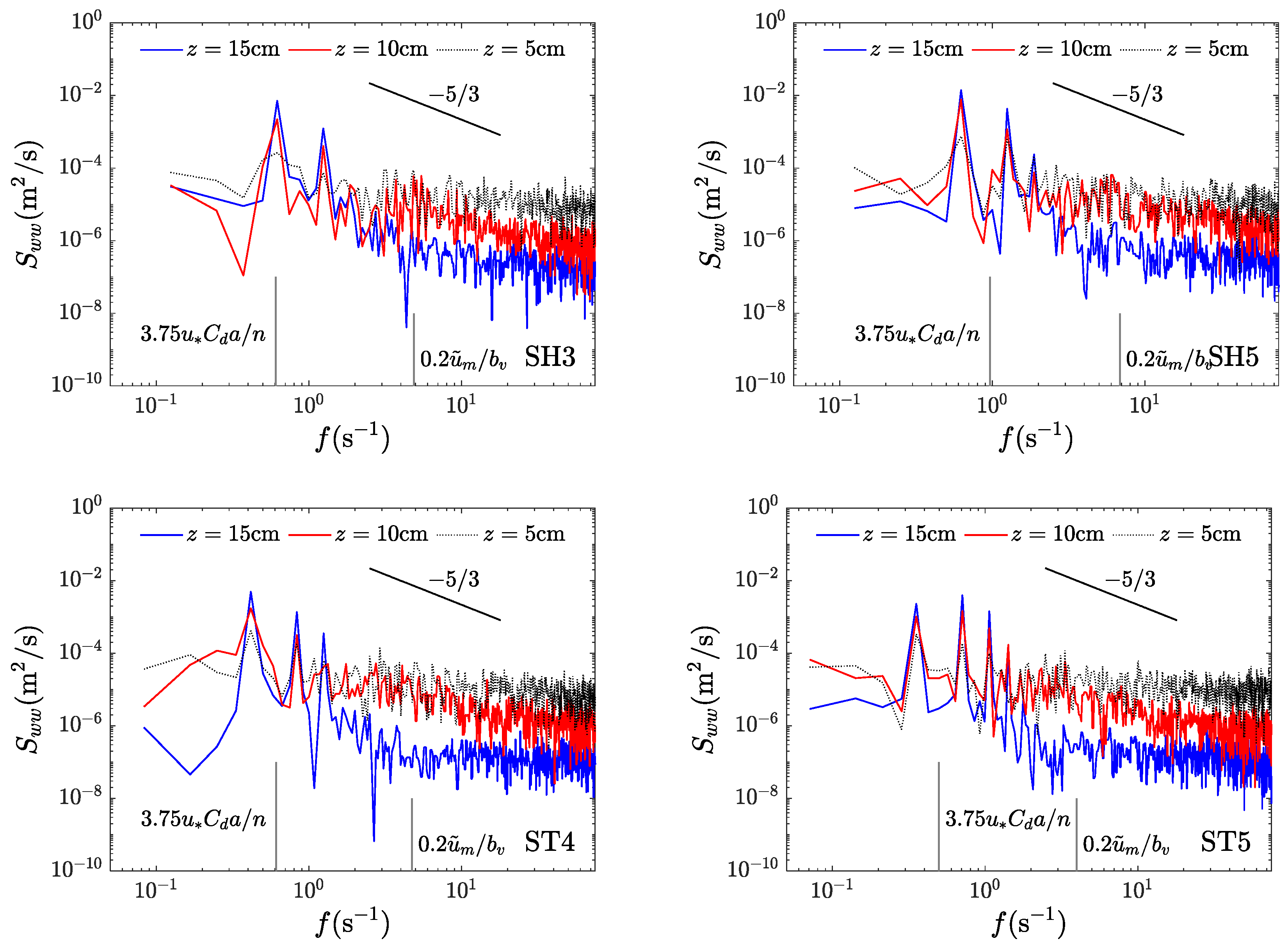
2.3. Analysis of Wake-Scale Turbulence

It is obvious that in the free fluid region, i.e., $n=$ 1 and $c_d=$ 0, the total $〈k〉-〈\epsilon 〉$ equations return to the original $〈k_s〉-〈{\epsilon }_s〉$ equations. Additionally, it should be noted that, without the consideration of a spectral shortcut, the commonly adopted $〈k〉$ equation in Equation (A1) [21,29,30,38,46] could be obtained by the superposition of Equations (10) and (12).

As listed in

Table A1. Formulas of additional vegetation terms in $〈k〉-〈\epsilon 〉$ model.

Model	${\mathit{P}}_{\mathit{w}}$	${\mathit{D}}_{\mathit{w}}$
LG [21,29,30]	$P_w^{\ast }$	$C_{\epsilon 1}{C}_{f\epsilon }{P}_w^{\ast }{\displaystyle \frac{〈\epsilon 〉}{〈k〉}}$
Liu [46]	$P_w^{\ast }$	${\displaystyle \frac{C_{\epsilon 2}}{\gamma }}{f}_1\left({\displaystyle \frac{P_s}{P_w^{\ast }}}\right){P_w^{\ast }}^{{\displaystyle \frac{4}{3}}}{b}_v^{-{\displaystyle \frac{2}{3}}}$
Tang [38]	$\sqrt{f_2\left({\displaystyle \frac{P_s}{P_w^{\ast }}}\right)}{P}_w^{\ast }$	${\displaystyle \frac{C_{\epsilon 2}}{\gamma }}{f}_2\left({\displaystyle \frac{P_s}{P_w^{\ast }}}\right){P_w^{\ast }}^{{\displaystyle \frac{4}{3}}}{b}_v^{-{\displaystyle \frac{2}{3}}}$

, the LG model was proposed by Shimizu and Tsujimoto [29], and then was used by López and García [30] and Ma et al. [21] under unidirectional flow and breaking wave conditions. To include the wake-scale turbulence, a modified formula of $D_w$ was presented in Liu et al. [46] and Tang et al. [38]. In the wake region, it is usually assumed that $P_w\approx 〈\epsilon 〉$ and the advection is negligible under the steady and uniform flow condition. The simplified $〈\epsilon 〉$ equation of Equation (A2) is as follows

$$D_w=C_{\epsilon 2}{\displaystyle \frac{{〈\epsilon 〉}^2}{〈k〉}}$$

(18)

Therefore, it could be found that the modeled $〈k〉$ in Tang et al. [38] strictly follows the relationship in Equation (1). It indicates that the significant suppression of wake-turbulence generation still results in a strong turbulence. Based on the assumption of wake scale in Equation (13), a clear reduction in wake-scale turbulence near the free end could be obtained by the presented model, which is expressed as follows:

$$〈k_w〉={\beta }_w^2{\left[f\left({\displaystyle \frac{P_s}{P_w^{\ast }}}\right){\displaystyle \frac{2\varphi }{\left(1-\varphi \right)\pi }}\right]}^{2/3}{〈u〉}^2$$

(19)

where ${\beta }_w$ is a new coefficient. The previous laboratory studies [19,47] have shown that the coefficient $\gamma$ in Equation (1) correlates with vegetation density and diameter. As discussed in the following section, the drag coefficient is also diameter-dependent. To eliminate the need for additional assumptions about the values of $C_d$ and $C_{fk}$, these three variables were combined into a single coefficient, defined as ${\beta }_w=\sqrt{\gamma }{\left(C_{fk}{C}_d\right)}^{1/3}$. For consistency with the solution for $〈k_w〉,$ given in Equation (19), the constants $C_{\epsilon D}$ and ${\beta }_w$ must be related by the following:

$$C_{\epsilon D}={\displaystyle \frac{C_{fk}}{{\beta }_w^3}}$$

(20)

When the shear-scale turbulence exerts a relatively weak suppression on wake generation, $f\left(P_s/P_w^{\ast }\right)=$ 1, and Equation (19) returns to Equation (1). It is noted that the suppression of WKE at the vegetation top leads to a corresponding reduction in Reynolds stress, thereby slightly enhancing the onshore current.

2.4. Boundary Conditions and Numerical Scheme

Appropriate boundary conditions are essential for solving the governing equations. In the present model, the two-phase volume of fluid (VOF) method [48] was used to track the water–air interface and a zero-stress condition was applied at the free surface by neglecting the influence of air flow (${\tau }_{ij}=0$). For the mean flow model, a no-slip boundary condition was imposed on the sea floor. In the turbulence model, the log-law distribution of mean tangential velocity within the turbulent boundary layer was applied to the grid point immediately above the sea floor. Additionally, zero-gradient boundary conditions were imposed for both SKE $〈k_s〉$ and WKE $〈k_w〉$, as well as their respective dissipation rates, $〈{\epsilon }_s〉$ and $〈{\epsilon }_w〉$, at the free surface (i.e., $\partial 〈k〉/\partial \overrightarrow{n}=\partial 〈\epsilon 〉/\partial \overrightarrow{n}=0$). In this study, the internal wave-maker method developed by Lin and Liu [49] was employed to generate the desired wave conditions. The model was executed for each case over 100 wave periods and 100 s under wave and current conditions, respectively. Only the final 50 wave periods and 50 s were considered for analysis. To ensure that waves reach a quasi-steady state, numerical sponge layers and radiation boundaries were applied on both lateral sides of the domain to absorb outgoing waves and prevent reflection.

In the numerical model, the same nonuniform discretization with a minimum ${∆x}_{\mathrm{m}\mathrm{i}\mathrm{n}}=$ 0.01 m and ${∆z}_{\mathrm{m}\mathrm{i}\mathrm{n}}=$ 0.002 m in the vegetation region was applied for both validations and current simulations. To ensure computational stability, both the Courant–Friedrichs–Lewy condition (Equation (22)) and the diffusive limit condition (Equation (23)) were used to automatically adjust the time step.

$$∆t\le {\alpha }_1·\min \left({\displaystyle \frac{∆x}{{\left|u\right|}_{\mathrm{m}\mathrm{a}\mathrm{x}}}},{\displaystyle \frac{∆z}{{\left|v\right|}_{\mathrm{m}\mathrm{a}\mathrm{x}}}}\right)$$

(21)

$$∆t\le {\alpha }_2·{\displaystyle \frac{1}{2\left(\upsilon +{\upsilon }_t\right)}}{\left[{\displaystyle \frac{1}{1/{\left(∆x\right)}^2+1/{\left(∆z\right)}^2}}\right]}^{1/2}$$

(22)

where ${\left|u\right|}_{\mathrm{m}\mathrm{a}\mathrm{x}}$ and ${\left|v\right|}_{\mathrm{m}\mathrm{a}\mathrm{x}}$ are the maximum flow velocities, and the empirical coefficients are ${\alpha }_1={\displaystyle \frac{3}{10}}$ and ${\alpha }_2={\displaystyle \frac{2}{3}}$ in this study.

3. Laboratory Experiments

3.1. Experimental Setup

Laboratory experiments were carried out at Hohai University in a glass-walled wave channel, which is 50 m long, 0.5 m wide and 1.5 m high. The transparent sidewalls allowed for easy introduction of light or laser beams to visualize and record the flow area. Waves were generated upstream using a hydraulic piston-type wave maker. To minimize wave reflection, a 15 m long mild slope was installed at the downstream end of the flume, covered with dense sponge filter sheets to gradually dissipate wave energy.

Velocity measurements around the vegetation were obtained using the 2-D PIV method. The flow was seeded with silver-coated particles with a diameter of 10 $\mu \mathrm{m}$. As shown in Figure 1a, the field of view (FOV) was centered on the vegetation patch to minimize sidewall effects. A thin laser sheet, produced by an LD Pumped All-Solid-State Green Laser (MGL-W-532), was introduced vertically into the FOV through a transparent acrylic lid to illuminate the flow field. The arrangement of 3 vertical laser light sheets (LLSs) is shown in Figure 1b. For each test, images of the illuminated area were captured using a Photron high-speed camera (Mini WX50), with frame sizes of 400 mm × 200 mm and 200 mm × 200 mm, providing a spatial resolution of 0.19 mm/pixel at 250 and 500 frames per second (fps), respectively. The minimum interrogation window size was set to 8 pixels [50]. As a result, the fps was set to 250 for smaller wave heights and shorter periods (cases SH1–3 and ST1–2) and 500 fps for other tests.

In this study, a 2.0 m long wooden vegetation model, covering the entire width of the wave flume, was equipped at the center of the wave flume. Coordinate $z$ was defined as the vertical distance from the seabed. Each vegetation stem had a diameter of $b_v=$ 6 mm and a length of $l=$ 0.1 m. The vegetation density was $N_v=$ 1936  stems/m², with a spacing of $S=$ 3.8$b_v$, corresponding volume fraction of 5.5%. The frontal area per unit ground area was $al=$ 1.16, which is significantly greater than 0.1, indicating that the vegetation is dense enough to neglect dispersive stress [20]. The water depth was maintained at 0.3 m, resulting in a submerged ratio $l/d=$ 0.3. The 13 detailed wave conditions for the experiments are listed in

Table 1. List of tested wave conditions.

CASE	H (cm)	T (s)	${\mathit{C}}_{\mathit{d}}$	${\tilde{\mathit{u}}}_{\mathbf{\infty }}^{\mathbf{r}\mathbf{m}\mathbf{s}}$ (cm/s)	${\mathit{\alpha }}_{\mathit{w}}$	${\mathit{u}}_{\ast }$ (cm/s)	${\mathsf{\delta }}_{\mathit{e}}$ (cm)
SH1	3.8	1.6	0.28	6.3	0.82	$1.38(\pm$0.18)	$2.29(\pm$0.65)
SH2	5.2	1.6	0.36	9.2	0.84	$2.05(\pm$0.23)	$2.95(\pm$0.47)
SH3	7.3	1.6	0.50	11.8	0.89	$2.59(\pm$0.33)	$3.09(\pm$0.73)
SH4	9.4	1.6	0.69	14.3	0.91	$2.64(\pm$0.26)	$3.00(\pm$1.04)
SH5	11.0	1.6	0.64	17.7	0.83	$3.04(\pm$0.56)	$3.46(\pm$0.47)
ST1	6.7	1.2	1.35	10.3	0.78	$2.90(\pm$0.29)	$2.82(\pm$0.11)
ST2	7.4	1.6	0.44	11.7	0.89	$2.58(\pm$0.59)	$2.95(\pm$0.56)
ST3	6.3	2.0	0.38	11.8	0.88	$2.34(\pm$0.52)	$3.26(\pm$0.62)
ST4	6.4	2.4	0.46	10.8	0.93	$2.45(\pm$0.50)	$2.90(\pm$0.18)
ST5	6.4	2.8	0.45	10.4	0.86	$2.71(\pm$0.79)	$3.05(\pm$0.26)
ST6	7.0	3.2	0.52	10.4	0.92	$2.88(\pm$0.52)	$3.31(\pm$0.64)
ST7	7.4	3.6	0.39	11.0	0.95	$2.65(\pm$0.44)	$2.75(\pm$0.31)
ST8	5.5	4.0	0.55	9.1	0.90	$2.60(\pm$0.53)	$3.41(\pm$0.75)

The value in brackets indicate 95% confidence intervals.

. The wave Reynolds number, based on the vegetation diameter, ranged from $\mathrm{R}\mathrm{e}={\tilde{u}}_m{b}_v/\nu =$ 430–1250, and the Keulegan–Carpenter number was $KC={\tilde{u}}_{m}T/b_v=$ 20–90.

3.2. Data Analysis

Due to the close frequency between wave motion and turbulent fluctuations, it is challenging to separate the wave orbital velocities from turbulent fluctuations, especially in the vegetation zone. To address this, the velocity measured by PIV was filtered by a tenth-order Butterworth filter with wave frequency as the cutoff frequency. The velocities ${\tilde{u}}_{\infty }^{\mathrm{r}\mathrm{m}\mathrm{s}}$ at interface $z=l$, as shown in Table 1, were fitted by the rms velocity above the vegetation, following the relationship ${{\tilde{u}}_{\infty }^{\mathrm{r}\mathrm{m}\mathrm{s}}}_{\left(z\right)}\propto \cosh \left(kz\right)$, where $k$ is the wave number [4]. The attenuation of oscillatory velocity within vegetation ${\alpha }_w$ was defined by Lowe et al. [4] as ${\tilde{u}}^{\mathrm{r}\mathrm{m}\mathrm{s}}/{\tilde{u}}_{\infty }^{\mathrm{r}\mathrm{m}\mathrm{s}}$, where ${\tilde{u}}^{\mathrm{r}\mathrm{m}\mathrm{s}}$ represents a vertical average rms velocity within vegetation. As direct pressure measurements were unavailable, the pressure gradient was estimated from the momentum budget far above the vegetation, with the wave-driven pressure gradient approximated using linear wave theory as $\partial 〈p〉/\partial x\propto \cosh \left(kz\right)$. Additionally, the quadratic drag law was applied, and the drag coefficient $C_d$ was calibrated using the momentum budget deep within vegetation.

The depth of the penetration shear layer ${\mathsf{\delta }}_e$, listed in Table 1, was defined as the depth where wave-averaged shear stress decays to 10% of its maximum. In the present experiments, the shear layer was approximately 0.3$l$, and the friction velocity was subsequently estimated by the following:

$$u_{\ast }=\sqrt{{\displaystyle \frac{1}{T}}{\int }_0^T\left|{〈\overline{u^{\prime }{w}^{\prime }}〉}_{z=0.85l}\right|\mathrm{d}t}$$

(23)

The velocity records were also used to explore key terms in TKE budget. Phase-dependent TKE was calculated by $〈k〉=1.33/2\left(〈{u^{\prime }}^2〉+〈{w^{\prime }}^2〉\right)$. Wake production was estimated as

$$P_w=-〈{\overline{u_i^{\prime }{u}_j^{\prime }}}^{″}{\displaystyle \frac{\partial u_i^{″}}{\partial x_j}}〉$$

(24)

The wave-averaged shear production just above vegetation was calculated in the vertical by

$$P_s={〈\overline{u^{\prime }{w}^{\prime }}〉}_{\mathrm{m}\mathrm{a}\mathrm{g}}{\displaystyle \frac{\mathrm{d}{U}_0}{\mathrm{d}z}}$$

(25)

where ${〈\overline{u^{\prime }{w}^{\prime }}〉}_{\mathrm{m}\mathrm{a}\mathrm{g}}$ was the magnitude of Reynolds stress for the entire wave, the maximum orbital velocity was $U_0\left(z\right)=\sqrt{2}{\tilde{u}}_{\left(z\right)}^{\mathrm{r}\mathrm{m}\mathrm{s}}$ and the velocity gradient was obtained by central difference. To calculate the dissipation rate $\epsilon$, the asymptotic analysis derived by Lumley and Terray [51] was adopted in the present study. The vertical velocity was used here to minimize spectral leakage of the turbulent spectrum.

$$S_{ww}={\displaystyle \frac{7}{9}}\mathsf{\Gamma }\left({\displaystyle \frac{1}{3}}\right)A{\epsilon }^{2/3}{U}_{\mathrm{o}\mathrm{r}\mathrm{b}}^{2/3}{\left(4\pi f\right)}^{-5/3}$$

(26)

where $A=$ 0.5 is the universal Kolmogorov constant, $U_{\mathrm{o}\mathrm{r}\mathrm{b}}$ is $\sqrt{2}{{\tilde{u}}_{\infty }^{\mathrm{r}\mathrm{m}\mathrm{s}}}_{\left(1.5l\right)}$, $f$ denotes frequency and $\mathsf{\Gamma }$ denotes the gamma function.

4. Results

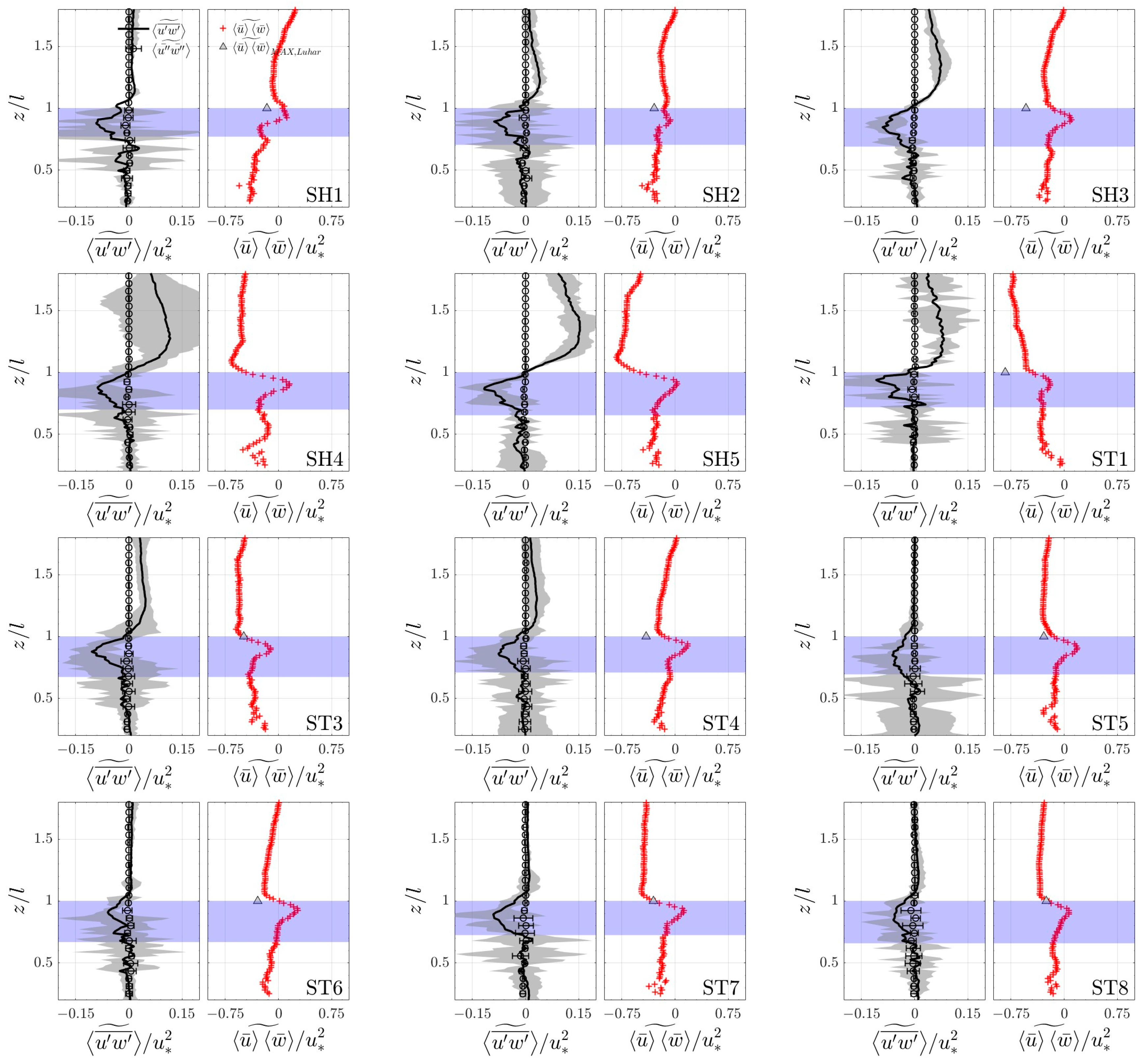
4.1. Wave and Turbulent Reynolds Stress

The vertical profiles of wave-averaged turbulent Reynolds stress $\widetilde{〈\overline{u^{\prime }{w}^{\prime }}〉}$, dispersive stress $\stackrel{~}{〈{\overline{u_i}}^{″}{\overline{u_j}}^{″}〉}$, and wave Reynolds stress $\widetilde{〈\overline{u}〉〈\overline{w}〉}$ are illustrated in Figure 2. The blue-shaded area indicates the thickness of the shear layer within the vegetation, while the gray-shaded area and error bars denote the 95% confidence intervals for turbulent Reynolds stress and dispersive stress, respectively. For all the present experiments, $al>$ 0.1, the dispersive stress is obviously smaller than the turbulent Reynolds stress. Slight negative dispersive stress $\stackrel{~}{〈{\overline{u_i}}^{″}{\overline{u_j}}^{″}〉}$ was observed only near the top of the vegetation due to spatial inhomogeneity. As shown in Figure 2, the gradient of wave Reynolds stress serves as the primary driving force near the vegetation top, while the gradient of turbulent Reynolds stress contributes only a minor fraction, approximately 15% of the former. Dispersive stress, in turn, accounts for less than 5% of the turbulent Reynolds stress and is therefore negligible in comparison, particularly in dense vegetation.

The vertical distribution of turbulent Reynolds stress $\widetilde{〈\overline{u^{\prime }{w}^{\prime }}〉}$ is consistent across all cases. It is obvious that a wave boundary layer forms just above the vegetation, with turbulent Reynolds stress increasing towards the vegetation top. In contrast, the decline in wave Reynolds stress $\widetilde{〈\overline{u}〉〈\overline{w}〉}$ above the vegetation suggests a balance between turbulent and wave Reynolds stress in the free stream region. A sharp decrease in $\widetilde{〈\overline{u^{\prime }{w}^{\prime }}〉}$ occurs near the top of the vegetation, while an opposite trend was observed in the wave Reynolds stress $\widetilde{〈\overline{u}〉〈\overline{w}〉}$, suggesting that turbulent Reynolds stress $\widetilde{〈\overline{u^{\prime }{w}^{\prime }}〉}$ at the interface of the vegetation and upper free water suppresses the generation of onshore current. As shown in Figure 2, the turbulent Reynolds stress $\widetilde{〈\overline{u^{\prime }{w}^{\prime }}〉}$ is much smaller than the wave Reynolds stress $\widetilde{〈\overline{u}〉〈\overline{w}〉}$, indicating that $\widetilde{〈\overline{u}〉〈\overline{w}〉}$ serves as the primary driving force for wave-induced flow at the vegetation top. Although two-point measurements confirmed that reflected wave energy was below 5%, residual wave reflection within the closed flume still introduces periodic variations in $\widetilde{〈\overline{u}〉〈\overline{w}〉}$. The periodicity results in two distinct vertical distributions—either increasing or decreasing from the bed—depending on the wave period or wavelength at a fixed measurement location. However, for identical wave periods (e.g., SH1, SH2, SH3), $\widetilde{〈\overline{u}〉〈\overline{w}〉}$ consistently increases from the bed, highlighting the robustness of the distribution under controlled conditions. It is obvious that the vegetation patch substantially alters the vertical structure of wave Reynolds stress. Sharp gradients in wave-induced Reynolds stress $\widetilde{〈\overline{u}〉〈\overline{w}〉}$ occur at the vegetation–flow interface, which drive the formation of a pronounced jet-like current along this boundary. For reference, the wave Reynolds stress predicted by Luhar et al. [52] at the top of the vegetation is also presented in Figure 2. Although their model overestimates the magnitude of wave Reynolds stress $\widetilde{〈\overline{u}〉〈\overline{w}〉}$ for cases SH3, SH4, SH5, ST1, and ST2, it accurately predicts results for the others, indicating that wave energy transferred from the free-stream region into the vegetation is mainly dissipated through vegetation drag. Despite the large uncertainty in SH2, ST2, and ST5 below the penetrative shear layer $\left(z<l-{\mathsf{\delta }}_e\right)$, the turbulent Reynolds stress tends to approach zero, indicating minimal impact on the wave-averaged flow far from the penetrative shear layer.

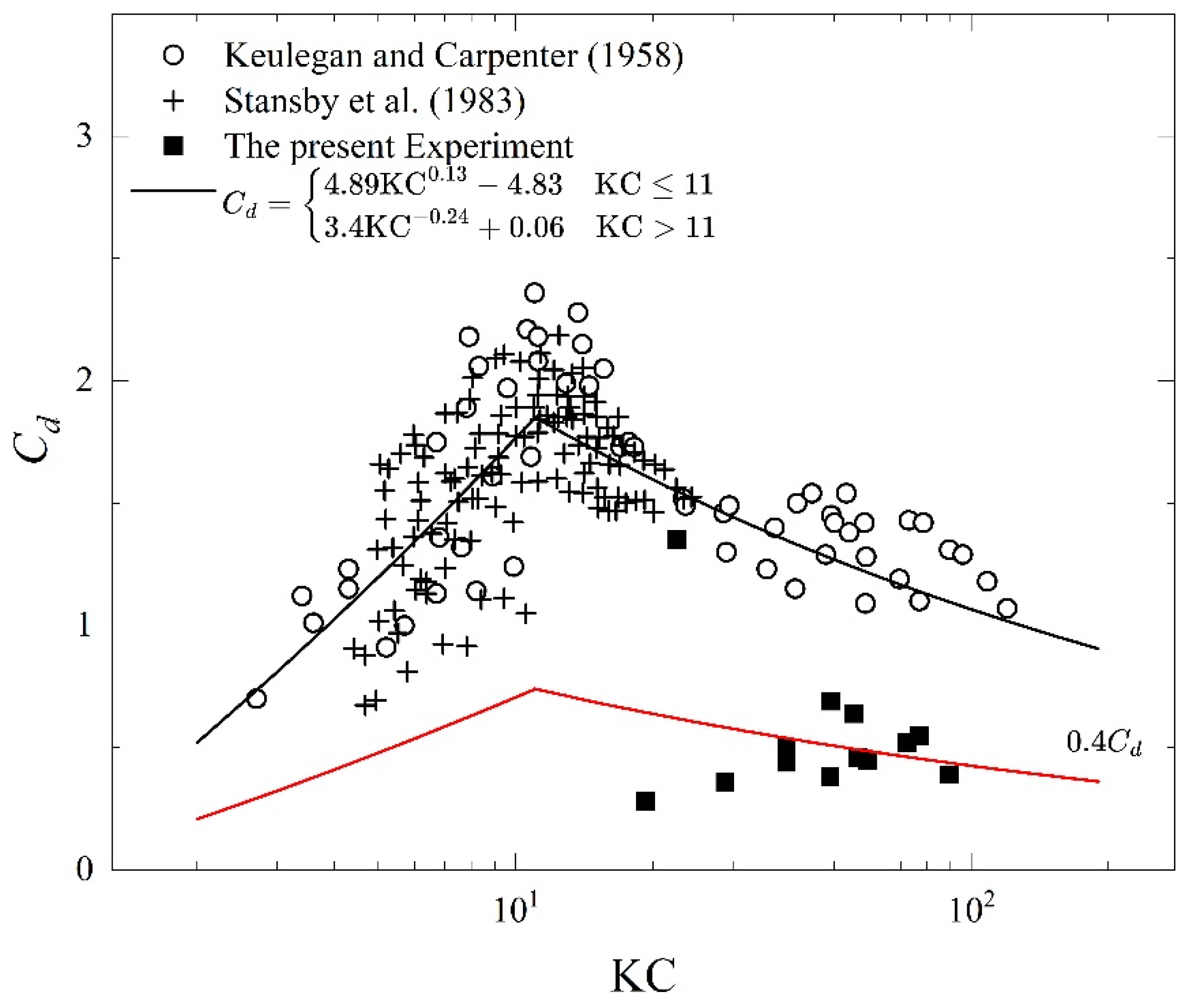
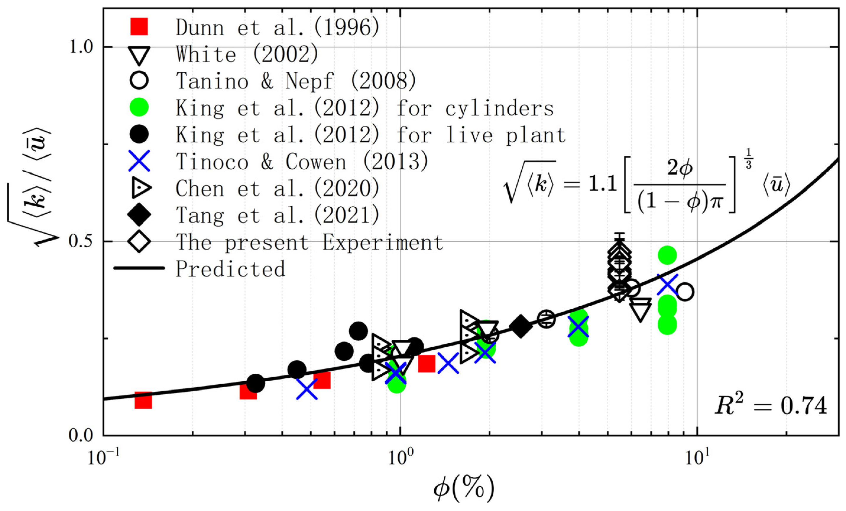
4.2. Drag Coefficient

Under wave conditions, the drag coefficient of the vegetation was found better correlated with the KC number [53]. Keulegan and Carpenter [54] and Stansby et al. [55] measured the drag coefficient of a quasi-2-D vertical cylinder in oscillatory flow. It is clear that KC = 11 marks a critical point. Numerical simulations by An et al. [56] on oscillatory flow around a circular cylinder at a constant Reynolds number of 2000 revealed that as KC increases, a transverse vortex street forms, with the attached vortex creating a significant negative pressure zone on the cylinder surface, thereby amplifying drag forces and increasing the drag coefficient from 0.7 to 2.36. However, when KC exceeds 11, the transverse vortex street vanishes, and the shed vortices align parallel to the oscillatory flow direction, resembling the vortex shedding pattern observed in steady flow. Consequently, in this regime, the drag coefficient remains relatively stable and converges toward its steady-flow value. Therefore, the drag coefficient was fitted separately for the two regimes divided at KC = 11. The empirical formula for the drag coefficient away from the cylinder tips could be expressed as

$$C_d=\left\{\begin{array}{cc}4.89{\mathrm{K}\mathrm{C}}^{0.13}-4.83& \mathrm{K}\mathrm{C}\le 11\\ 3.4{\mathrm{K}\mathrm{C}}^{-0.24}+0.06& \mathrm{K}\mathrm{C}>11\end{array}\right.$$

(27)

with a coefficient of determination R² of 0.67. It is noted that for $\mathrm{K}\mathrm{C}\le$11, R² is slightly lower at 0.55, whereas for $\mathrm{K}\mathrm{C}>$11, the fit of Equation (27) improves, reaching an R² value of 0.76. For cylindrical arrays, the upstream wake has a significant influence on the drag coefficient. Intense turbulence within the vegetation further reduces the drag coefficient. As shown in Figure 3, a sheltering factor $k_N=$ 0.4 was applied, yielding a root mean square error (RMSE) of 0.25.

To quantify the effect of tips on the drag coefficient, Figure 4 presents the phase distributions of key dimensionless momentum terms, including the inertial term $\partial 〈\overline{u}〉/\partial t+f_I$, the pressure gradient term $\partial 〈\overline{p}〉/\partial x$, the drag force $f_d$, and the advection terms $\partial {〈\overline{u}〉}^2/\partial x$ and $\partial 〈\overline{u}〉〈\overline{w}〉/\partial z$. These terms were non-dimensionalized by $\omega {\tilde{u}}_{\infty }^{\mathrm{r}\mathrm{m}\mathrm{s}}$ for consistency. The phase reference $\left(\theta =0^{°}\right)$ was defined as the moment when the horizontal velocity at $z/l=$ 1.5 crosses zero. It is noted that the drag force shown in Figure 4 was derived as the residual of the momentum budget. The results indicate that the primary balance is between the inertial and pressure gradient terms. However, due to the modulation of horizontal velocity within the vegetation, the drag force also plays a significant role in momentum balance. Although turbulent Reynolds stress is not displayed, it was found to be much smaller than other momentum terms. Below the penetrative shear layer, these results align with the scaling relationship proposed by Zeller et al. [35], expressed as unsteadiness $~$ pressure $\gg$ drag $\gg$ advection, turbulent Reynolds stress. This suggests that within vegetation, drag is primarily balanced by unsteadiness and pressure, while the drag coefficient remains nearly constant.

In the penetrative shear layer, the advection term becomes non-negligible, intensifying the drag force and suggesting a local relationship of drag$~$advection. This behavior resembles that observed in a single cylinder with free end, where three-dimensional vorticity near the tip significantly reduces base pressure [57]. Additionally, the drag force induced by advection could also be effectively modeled using quadratic drag laws, such as the oscillatory pattern similar to that below the penetrative shear layer in Figure 4.

As the influence of the tips decreases toward the vegetation base, the drag coefficient approaches that of an infinitely long cylinder. Accordingly, the drag force distribution along the vegetation height is divided into two distinct regions: (1) an upper region dominated by free-end effects, and (2) a lower region governed by a periodic vortex-shedding process. The extent of the unaffected region, denoted $l^{2D}/b_v$, is a function of $l/b_v$ [58]. Figure 5 shows the fitted height of the two-dimensional wake-dominated region $l^{2D}/b_v$ and the profile of drag coefficient. Based on a statistical analysis of experimental results from previous studies [26,31,34,58,59,60,61,62], the drag coefficient in dense submerged vegetation up to $\varphi =$ 5.5% is still similar to that for a single cylinder, and the relationship between $l^{2D}/b_v$ and $l/b_v$ is expressed as in [58]

$${\displaystyle \frac{l^{2D}}{b_v}}=0.097{\left({\displaystyle \frac{l}{b_v}}\right)}^{1.78}$$

(28)

The vertical distribution of the normalized drag coefficient $C_{d\left(z\right)}/C_d$ is given by

$${\displaystyle \frac{C_{d\left(z\right)}}{C_d}}=\left\{\begin{array}{cc}-2.3{\displaystyle \frac{z-l^{2D}}{l^{3D}}}+3.5& \left(z-l^{2D}\right)/l^{3D}\ge 0.6\\ 1.8\mathrm{e}\mathrm{x}\mathrm{p}\left[-{\left({\displaystyle \frac{\frac{z-l^{2D}}{l^{3D}}-1}{0.64}}\right)}^2\right]+1.04\mathrm{e}\mathrm{x}\mathrm{p}\left[-{\left({\displaystyle \frac{\frac{z-l^{2D}}{l^{3D}}+2.4}{8.2}}\right)}^2\right]& \left(z-l^{2D}\right)/l^{3D}<0.6\end{array}\right.$$

(29)

The peak drag coefficient is observed at $\left(z-l^{2D}\right)/l^{3D}=$ 0.6, which corresponds to $z/l\approx$ 0.96 in the present experiments. At this position, the advection term indicates significant local horizontal pressure gradients, which are modeled as drag forces. It is noted that the drag profile shows a great agreement for vegetation arranged in rectangular [34] and staggered [31] configurations. According to data from Tang et al. [34] and O’Donncha et al. [31], the maximum drag coefficient occurs at 0.8$l$ and 0.76$l$ for aspect ratios of 10 and 10.48, aligning closely with the values predicted by Equations (28) and (29), which yield 0.83$l$ and 0.84$l$. It is important to note that the local drag coefficient discussed here is derived from an analysis of the flow field near the vegetation. The drag profile also validated for randomly distributed vegetation arrays [26]. In the study by Ghisalberti and Nepf [26], adjacent plants were removed, and a 12.5$b_v$ long space was cleared to ensure sufficient space for measurements, where the flow field was nearly fully developed, leading to an approximately 40% reduction in the $l^{2D}$ value compared to the prediction given by Equation (28). The measured $l^{2D}$ from Ghisalberti and Nepf [26] was used to calculate $\left(z-l^{2D}\right)/l^{3D}$ in Figure 5. It is obvious that the drag profile remains consistent with experimental measures, even for random arrays of vegetation with solid volume fractions of $\varphi =$ 1.26–4.0%. The distribution of $C_{d\left(z\right)}/C_d$ clearly mirrors that of a single cylinder, with the maximum occurring at $\left(z-l^{2D}\right)/l^{3D}=$ 0.6, corresponding to 0.8$l$ which is in close agreement with the observed value of 0.76$l$. When the aspect ratio is reduced to 5, as in Okamoto and Yagita [60], the peak drag coefficient appears at 0.7$l$, closely matching the value predicted by the present model, which gives 0.73$l$. For short vegetation, where $l/b_v<$ 3.314, the influence of tips extends across the entire height. Conversely, when the vegetation is sufficiently tall, with $l/b_v>$ 19.9, the tip effects become negligible due to their limited influence.

The assumption of a constant shape for the drag coefficient is widely adopted due to the lack of consideration for tip effects. To assess the significance of tip effects in quantifying the drag coefficient, the spatial distribution of drag forces was fitted using both the constant coefficient assumption and the formulation in Equation (29). The ratio of their RMSE values was then defined as the index IRI.

$$\mathrm{I}\mathrm{R}\mathrm{I}={\displaystyle \frac{\mathrm{R}\mathrm{M}\mathrm{S}\mathrm{E}\left\{C_d\right\}}{\mathrm{R}\mathrm{M}\mathrm{S}\mathrm{E}\left\{C_{d_{\left(z\right)}}\right\}}}$$

(30)

Figure 6 compares the parameter IRI with the KC number. As shown in Figure 6, IRI remains largely insensitive to KC, with an overall value of 1.26 within the vegetation, indicating that neglecting tip effects slightly increases the prediction error of the drag coefficient. As illustrated in Figure 5b, in regions far away from the vegetation top $\left(z-l^{2D}\right)/l^{3D}<$ −0.328, where tip effects are minimal, the drag coefficient remains approximately constant, resulting in an IRI value of 1.0 in Figure 6. In contrast, near the vegetation top, IRI increases significantly, peaking at 1.45, indicating that the formulation incorporating tip effects (Equation (29)) provides a more accurate prediction than the constant-coefficient assumption.

The amplification of the drag coefficient at the free end is primarily attributed to the advection term. As shown in Figure 2, wave Reynolds stress plays a critical role near the top of the vegetation. It is essential to further explore the role of this nonuniform drag coefficient in wave-averaged momentum balance. Within the vegetation, the force balance is dominated by shear stress gradient, along with the mean drag [14].

$${\displaystyle \frac{\partial {\tilde{\tau }}_{xz}}{\partial z}}=\widetilde{f_d}$$

(31)

Both terms in Equation (30) were computed and plotted in Figure 7. The shear stress gradient $\partial {\tilde{\tau }}_{xz}/\partial z$ consists of the gradients of wave and turbulent Reynolds stresses, $\partial \widetilde{〈\overline{u}〉〈\overline{w}〉}/\partial z$ and $\partial \widetilde{〈\overline{u^{\prime }{w}^{\prime }}〉}/\partial z$, respectively. Under wave-dominated conditions, the assumption that the mean current velocity at the top of the vegetation ($z=l$) is much smaller than the oscillatory wave velocity amplitude ($〈u_c〉/〈u_m〉\ll 1$) remains valid. Thus, the wave-averaged drag is primarily generated by wave–current interactions, and its magnitude could be expressed as

$$\widetilde{f_d}~{\displaystyle \frac{2\sqrt{2}}{\pi }}{C}_{d}a{\tilde{u}}_{\infty }^{\mathrm{r}\mathrm{m}\mathrm{s}}〈u_c〉$$

(32)

In Figure 7, the wave-averaged velocity was non-dimensionalized by the maximum current velocity. The wave-averaged drag balances the two primary force contributions within the vegetation, the wave and turbulent Reynolds stress gradients, while these stress gradients counterbalance each other in the region above the vegetation. At the vegetation top, a discontinuity in drag force generates an onshore-directed flow. According to Equation (32), the corresponding wave-averaged drag $\widetilde{f_d}$ becomes negative and is predominantly balanced by the wave Reynolds stress $\widetilde{〈\overline{u}〉〈\overline{w}〉}$ as shown in Figure 2. Meanwhile, the opposing and increasing trend in turbulent Reynolds stress indicates that the gradient of $\widetilde{〈\overline{u^{\prime }{w}^{\prime }}〉}$ acts to suppress the generation of onshore transport near the vegetation top. Consistent with Figure 6, incorporating tip effects using the distribution form of Equation (29) significantly improves the accuracy of drag force, particularly near the top of the vegetation. As shown in Figure 7, neglecting tip effects results in underestimation of the wave-averaged drag when using a constant drag coefficient. In contrast, the drag predicted by Equation (29) provides a more accurate estimate. Notably, for $z/l\ge$ 0.85, the wave-averaged drag predicted by the variable drag coefficient is approximately twice that of the constant coefficient.

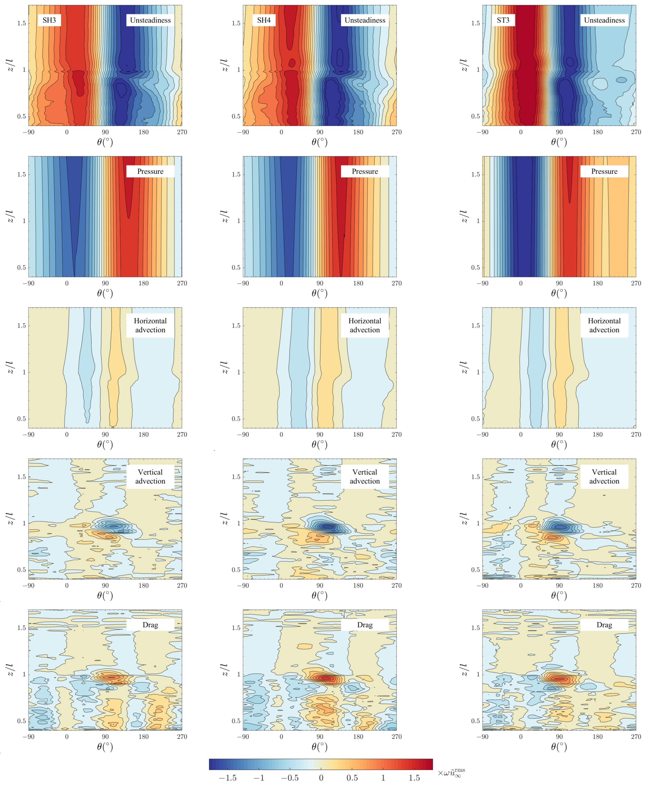
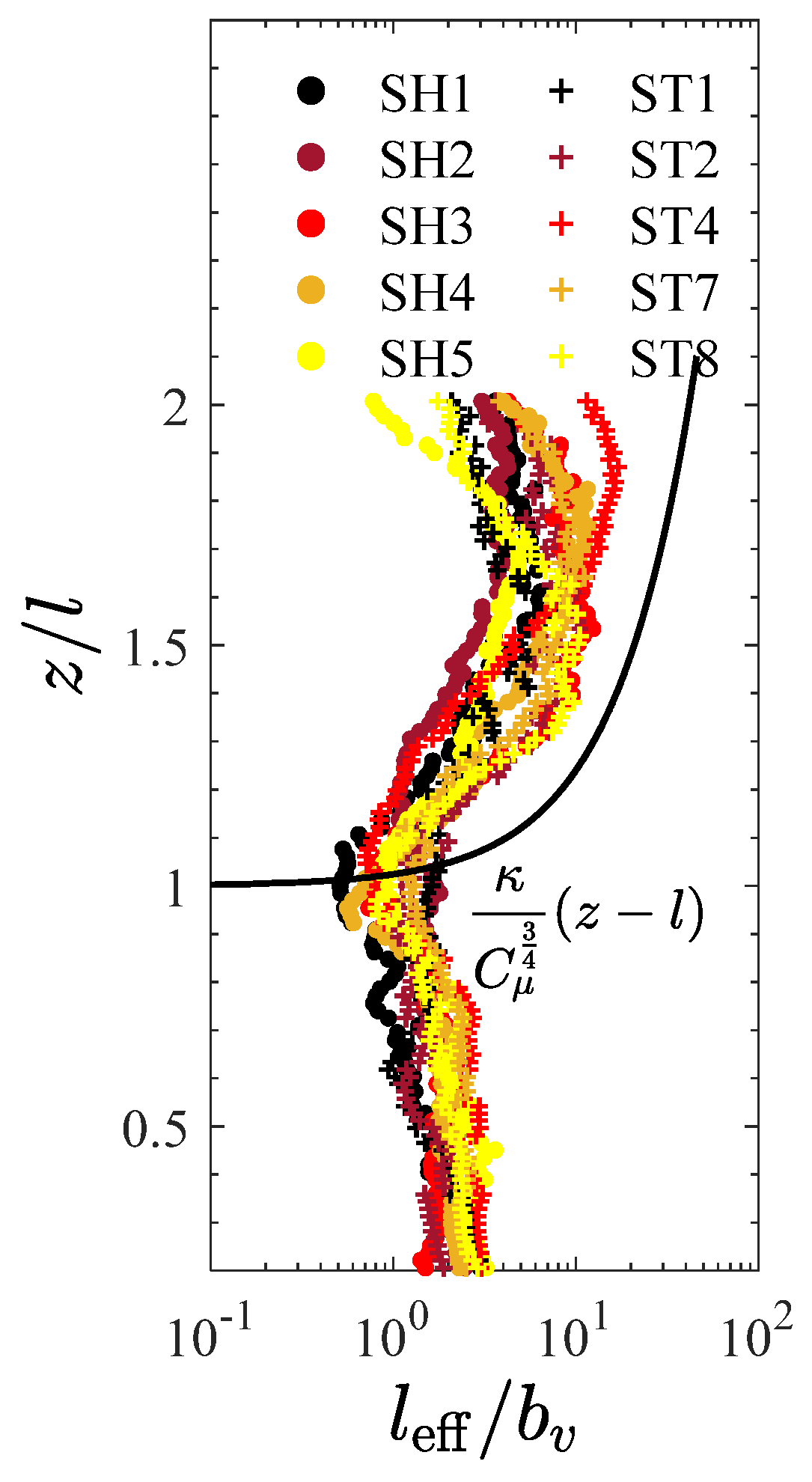
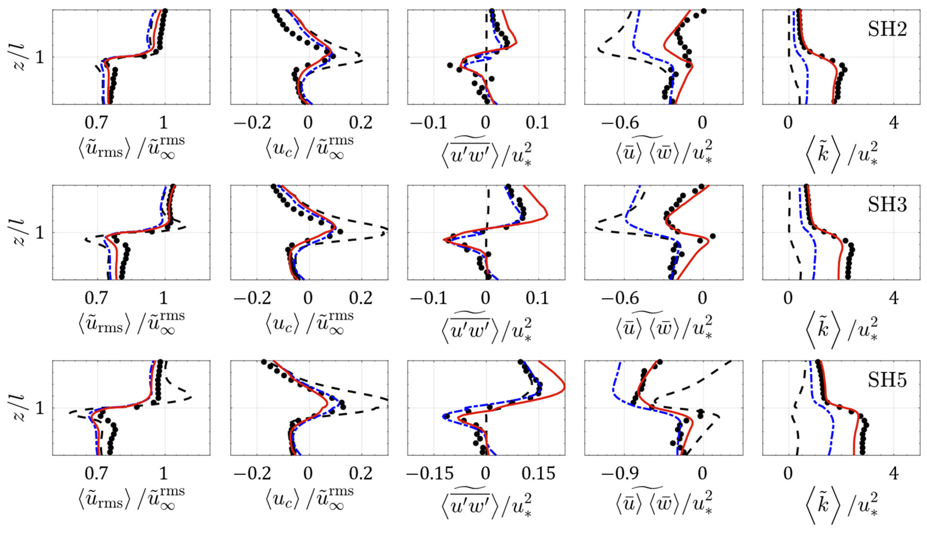
4.3. Turbulence Structure

The amplification of drag at the top of the vegetation was induced by the advection term, corresponding to the kinetic energy at wave frequencies. Consequently, the uniform distribution of drag coefficient $C_d$ was adopted in the wake production term, which was expressed as Equation (17). Figure 8 presents the coefficient distribution calculated by Equation (17). It is noted that the suppression effect becomes negligible, with $f\left(P_s/P_w^{\ast }\right)=$ 1, away from the penetrative shear layer, indicating that the conversion is more efficient with $C_{fk}=$ 1. However, a significant suppression of wake production also could be found around the top of the vegetation. It indicates that wake generation also shows significant suppression by the free end disturbance even in a wake dominated region. The parameter $P_s/P_w^{\ast }$ was used in the present study to quantify the intensity of the shear process near the top of the vegetation [38,46].

The near-wake flow behind finite-length vegetation is characterized by the coexistence and interaction of spanwise and tip vortices. In submerged vegetation, the shear generated at the top of the vegetation represents a significant source of shear production, confined to a region within 0.3$l$ from the top of the vegetation (Figure 2). As shear production becomes negligible at greater distances from the top, the coefficient $C_{fk}$ at a height of 0.5$l$ within the vegetation is considered the baseline for wake generation, i.e., $f\left(P_s/P_w^{\ast }\right)=$ 1. It is important to note that the shear production term, as calculated by Equation (25), is no longer applicable within the wake region. Consequently, only the three adjacent grid points near the tips were selected to obtain the parameter $P_s/P_w^{\ast }$. Figure 9 demonstrates the relationship between the suppression function and this parameter. For comparison, the suppression function proposed by Tang et al. [38], which applies in cases dominated by shear-generated turbulence, is also presented (solid black line). As shown in Figure 8 and Figure 9, the free-end effects significantly influence wake generation. Flow visualizations from Wang and Zhou [63] reveal the formation of Kelvin–Helmholtz vortices in the separated shear layer, while the descending motion of the free-end shear layer disrupts wake structures in the (x, y) plane. This emphasizes the critical influence of tip shear intensity on the development of wake-scale vortices. It is evident that, even when the parameter is small ($P_s/P_w^{\ast }\approx$ 0.1), the suppression of wake turbulence generation remains significant, with the suppression function value $f\left(P_s/P_w^{\ast }\right)$ as low as 0.6 or even lower. In contrast, the suppression function proposed by Tang et al. [38] clearly underestimates the effect of the tips on wake generation, predicting a suppression function value as high as 0.9.

Figure 10 presents the power spectra both above the vegetation ($z/l=$ 1.5), at the vegetation top ($z/l=$ 1.0) and within the vegetation ($z/l=$ 0.5), with the −5/3 slope and the Strouhal number 0.2${\tilde{u}}_m/b_v$ included for reference. To eliminate white noise, the high-frequency components above 75 Hz were truncated. In the low-frequency range corresponding to the incoming wave frequencies, the power spectra of the incident wave energy maintain high levels inside and outside the vegetation. At higher frequencies ($f>$ 1.2 Hz), the power spectra were higher at $z/l=$ 0.5 and gradually decrease toward the vegetation top ($z/l=$ 1.0) and the above free-stream region ($z/l=$ 1.5), indicating more intense turbulence within the vegetation. As shown in Figure 10, the power spectra above the vegetation closely follow the classical −5/3 slope, consistent with inertial subrange scaling in isotropic turbulence. Unlike the energy transfer solely through inertial cascade, the mean flow performs work against vegetation drag, converting MKE into WKE and heat. Therefore, it is obvious that a distinct bump along with a steeper local decay in Figure 10 above the −5/3 slope could be found around the Strouhal number 0.2${\tilde{u}}_m/b_v$, indicating the dominance of wake-scale turbulence. This feature suggests that wake production significantly contributes to the local TKE budget. Another mechanism acting on turbulent structures is the spectral shortcut $W$ [20,64], where spatial confinement facilitates a bypass of the inertial cascade, transferring energy directly from large eddies to wake-scale eddies. This continuous extraction of energy from the cascade violates the key assumptions of Kolmogorov’s −5/3 law. Assuming that the energy removed via spectral shortcut remains small relative to the total dissipation, Finnigan [64] proposed a modified spectral shape of the form $f^{-5/3}\mathrm{e}\mathrm{x}\mathrm{p}\left(f^{-2/3}\right)$, which predicts a sharper spectral decay near the Strouhal frequency while asymptotically converging to the −5/3 slope at high frequencies.

Figure 11 shows the vertical distribution of the integral length scale, calculated as $l_{\mathrm{e}\mathrm{f}\mathrm{f}}~{\widetilde{〈k〉}}^{3/2}/〈\epsilon 〉$. For reference, the logarithmic law was also plotted for the region above the vegetation. Although the above free-stream region exhibits high variability in integral length scale due to weak turbulence across different cases, the general trend suggests that the flow follows classic boundary layer behavior, dominated by large-scale shear vortices with an integral length scale proportional to water depth $\left(l_{\mathrm{e}\mathrm{f}\mathrm{f}}~z\right)$. Within the vegetation, the integral length scale is significantly smaller than that in the free-stream region, with a ratio of approximately $l_{\mathrm{e}\mathrm{f}\mathrm{f}}/b_v~$1–3. This observation aligns with measurements by Nepf [18], who reported $l_{\mathrm{e}\mathrm{f}\mathrm{f}}~b_v$, and it is further validated by numerical calibrations from King et al. [20], showing $l_{\mathrm{e}\mathrm{f}\mathrm{f}}\approx 2.98b_v$. The integral length scale remains closely proportional to the stem diameter, even near vegetation tips, suggesting that wake-scale turbulence remains a significant component of total TKE.

Figure 12 shows the comparison between $\sqrt{〈k〉}/〈\overline{u}〉$ and $\varphi$. For the present experiments, data were selected from a region away from the free end, specifically within the height range of 0.4$l-$0.7$l$. Only cases with $b_v/S_n<$ 0.56 from Tanino and Nepf [19] were included in Figure 12. The regression analysis indicated a constant value of ${\beta }_w$ at 1.1 in Equation (19), with R² = 0.74.

5. Discussions

The performance of the present model was compared to that of the LG model. Given that both the Liu and Tang models are based on the same fundamental assumption of wake-scale turbulence (as in Equation (1)), only the performance of the Tang model is presented here for comparison. The model was initially calibrated and tested against fully developed open-channel flow through submerged vegetation.

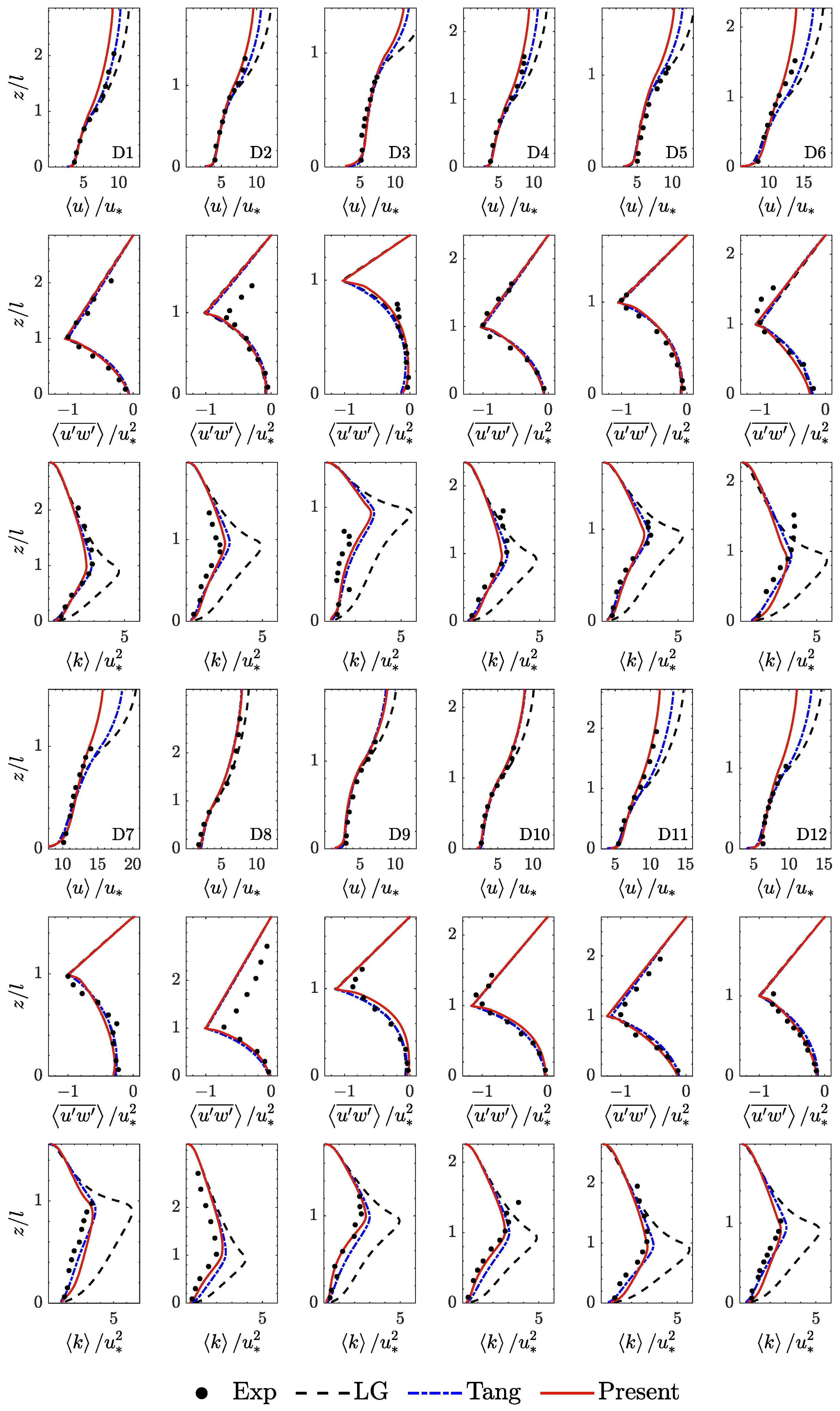
5.1. Validation with Unidirectional Flows

Two vegetation experiments listed in

Table 2. The parameters for validation cases under unidirectional flows.

Source	CASE	${\mathit{N}}_{\mathit{v}}$	${\mathit{b}}_{\mathit{v}}$ (mm)	$\mathit{l}$ (m)	$\mathit{d}$ (m)	$\mathit{S}$
King et al. [20]	S1	1290	3.1	0.193	0.257	0.00168
	S2	645	6.2	0.194	0.260	0.00203
	S3	315	12.7	0.193	0.257	0.00210
	S4	158	25.3	0.194	0.256	0.00082
	S5	1290	3.1	0.193	0.370	0.00015
	S6	645	6.2	0.194	0.367	0.00075
	S7	315	12.7	0.193	0.369	0.00012
	S8	158	25.3	0.194	0.368	0.00066
Dunn et al. [33]	D1	172	6.35	0.1175	0.335	0.00360
	D2	172	6.35	0.1175	0.229	0.00360
	D3	172	6.35	0.1175	0.164	0.00360
	D4	172	6.35	0.1175	0.276	0.00760
	D5	172	6.35	0.1175	0.203	0.00760
	D6	43	6.35	0.1175	0.267	0.00360
	D7	43	6.35	0.1175	0.183	0.00360
	D8	388	6.35	0.1175	0.391	0.00360
	D9	388	6.35	0.1175	0.214	0.00360
	D10	388	6.35	0.1175	0.265	0.01610
	D11	97	6.35	0.1175	0.311	0.00360
	D12	97	6.35	0.1175	0.233	0.01080

were used to validate the model. The first set, from King et al. [20], tested cylinders with diameters of [3.1, 6.2, 12.7 and 25.3] mm, fixed at densities of [1290, 645, 315 and 158] stems/m², corresponding to solid volume fractions of $\varphi =$ [0.97%, 1.95%, 3.99% and 7.94%], respectively. The second dataset from Dunn et al. [33] included cases with small solid volume fractions of $\varphi =$ [0.14%, 0.31%, 0.54% and 1.23%], and was also used for model validation.

For both cases, a nonuniform grid system with minimum sizes of ${∆x}_{\mathrm{m}\mathrm{i}\mathrm{n}}=$ 0.01 m and ${∆z}_{\mathrm{m}\mathrm{i}\mathrm{n}}=$ 0.001 m was used. Periodic boundary conditions were applied at the streamwise boundaries, with flow driven by an external pressure gradient $S$ depending on the experimental setup. The characteristic time scale, estimated to be 2.0 s (the time for water to flow through vegetation), was used to calculate the KC number and drag coefficient. The drag coefficient of 1.96 was selected in case S6 for all three models. For sparse vegetation ($\varphi \le$ 1.23%) with a gap-to-diameter ratio $S_n/b_v\ge$ 8 in Dunn et al. [33], the upstream wake had a limited effect on the drag coefficient, and a sheltering factor of $k_N=$ 1.0 was adopted.

To compare the present model with the two experiments listed in Table 2, the results are plotted in Figure 13, Figure 14 and Figure 15. The mean square errors (MSE), normalized by the variance of the measured vertical profile, are presented in

Table 3. Mean square errors for validation cases under unidirectional flows.

CASE	LG Model			Tang Model			The Present Model
	$〈\mathit{u}〉$	$〈\overline{{\mathit{u}}^{\mathbf{\prime }}{\mathit{w}}^{\mathbf{\prime }}}〉$	$〈\mathit{k}〉$	$〈\mathit{u}〉$	$〈\overline{{\mathit{u}}^{\mathbf{\prime }}{\mathit{w}}^{\mathbf{\prime }}}〉$	$〈\mathit{k}〉$	$〈\mathit{u}〉$	$〈\overline{{\mathit{u}}^{\mathbf{\prime }}{\mathit{w}}^{\mathbf{\prime }}}〉$	$〈\mathit{k}〉$
S1	0.10	0.10	2.25	0.10	0.04	0.19	0.03	0.06	0.25
S2	0.01	0.07	1.14	0.13	0.09	0.39	0.01	0.03	0.27
S3	0.01	0.08	1.50	0.19	0.14	0.52	0.11	0.04	0.23
S4	0.05	0.13	0.71	0.45	0.09	0.58	0.03	0.16	0.19
S5	0.03	0.18	0.85	0.03	0.13	0.20	0.05	0.13	0.26
S6	0.24	0.15	1.16	0.36	0.12	0.38	0.02	0.15	0.17
S7	0.03	0.39	1.07	0.48	0.42	0.63	0.17	0.12	0.13
S8	0.13	0.39	2.70	0.49	0.56	0.98	0.13	0.22	0.23
D1	0.06	0.06	2.68	0.01	0.06	0.06	0.10	0.05	0.21
D2	0.19	0.95	11.24	0.04	0.74	0.84	0.02	0.83	0.21
D3	0.10	1.81	38.05	0.14	2.55	4.52	0.14	0.96	1.46
D4	0.22	0.05	2.81	0.04	0.07	0.18	0.04	0.05	0.28
D5	0.07	0.02	2.46	0.09	0.02	0.02	0.25	0.04	0.14
D6	0.51	0.18	4.70	0.23	0.16	0.55	0.06	0.13	0.86
D7	0.40	0.07	15.57	0.33	0.06	0.47	0.07	0.10	0.19
D8	0.03	0.97	5.77	0.03	0.91	1.22	0.02	0.95	0.48
D9	0.04	0.08	4.11	0.05	0.07	0.29	0.06	0.12	0.08
D10	0.03	0.03	2.22	0.01	0.02	0.29	0.02	0.05	0.18
D11	0.55	0.13	6.00	0.20	0.10	0.24	0.02	0.12	0.20
D12	0.09	0.11	8.71	0.07	0.12	0.23	0.11	0.08	0.08
Average	0.14	0.31	5.79	0.17	0.32	0.64	0.07	0.22	0.31

.

The results for the three models, along with the experimental data from King et al. [20] and Dunn et al. [33] for small volume fractions ($\varphi <$ 2%) are presented in Figure 13 and Figure 15, respectively. The advantages of the present model were clear. While all three models accurately simulate $〈u〉$ and $〈\overline{u^{\prime }{w}^{\prime }}〉$, the LG model performs poorly in simulating $〈k〉$ with an average MSE of 5.79, clearly overestimating the TKE within vegetation. By incorporating the wake scale in $D_w$, the Tang model shows improved performance in simulating $〈k〉$, achieving an average MSE of 0.64. The present model also successfully predicts the vertical distribution of $〈k〉$, particularly its dependence on the wake scale within the vegetation.

Figure 13 compares the experimental data from King et al. [20] (with a large volume fraction, $\varphi$ > 2%) to the results simulated by three different models. It is evident that the Tang model deviates from the experimental data across all three variables. Specifically, it significantly underestimates the velocity $〈u〉$ above the vegetation. Furthermore, both the LG and Tang models, which neglect the tip effects, overestimate the Reynolds stress $〈\overline{u^{\prime }{w}^{\prime }}〉$ near the tips of the vegetation. Since SKE is a key component of the total TKE [17], the stronger shear production predicted by the Tang model leads to higher $〈k〉$ values, particularly near the upper free ends of the vegetation. Consequently, the Tang model is more appropriate for cases with $\varphi <$ 2%. In contrast, the present model consistently provides accurate predictions of $〈k〉$, with an average MSE of 0.31, making it a better choice for simulating cases involving dense, submerged vegetation.

The MSE for both the upper free stream and vegetation zones were also summarized in

Table 4. Mean square errors for validation cases for both the upper free stream and vegetation zones.

Zone	LG Model			Tang Model			The Present Model
	$〈\mathit{u}〉$	$〈\overline{{\mathit{u}}^{\mathbf{\prime }}{\mathit{w}}^{\mathbf{\prime }}}〉$	$〈\mathit{k}〉$	$〈\mathit{u}〉$	$〈\overline{{\mathit{u}}^{\mathbf{\prime }}{\mathit{w}}^{\mathbf{\prime }}}〉$	$〈\mathit{k}〉$	$〈\mathit{u}〉$	$〈\overline{{\mathit{u}}^{\mathbf{\prime }}{\mathit{w}}^{\mathbf{\prime }}}〉$	$〈\mathit{k}〉$
Free stream	0.28	0.40	1.62	0.36	0.33	0.49	0.14	0.32	0.38
In vegetation	0.05	0.20	6.95	0.05	0.28	0.65	0.04	0.12	0.38

. It is obvious that the LG model exhibits a significantly poor performance in predicting $〈k〉$ especially within the vegetation zone, with MSE values that are 10 and 18 times larger than those of the Tang model and the present model, respectively. While the Tang model improves $〈k〉$ prediction by incorporating the wake scale in $D_w$, its velocity MSE remains 2.5 times larger than that of the present model. Overall, the present model demonstrates superior predictive capability across all three variables, particularly within the vegetation zone, where the average MSEs are 0.04, 0.12 and 0.38, respectively.

5.2. Validation with Oscillatory Flows

The comparisons for the profiles of velocity; shear stress and TKE at the center of the vegetation patch between the three models and the present study’s experimental data are shown in Figure 16. Notably, the present model consistently outperforms the other two models in predicting wave Reynolds stress and TKE, with average MSEs of 0.58 and 0.09, respectively. It is obvious that the LG model tends to consistently underestimate $\widetilde{〈\overline{u^{\prime }{w}^{\prime }}〉}$, which leads to an overestimation of the onshore current near the free end of the vegetation. In contrast, the present model achieves better agreement with the measured values of $〈{\tilde{u}}_{\mathrm{r}\mathrm{m}\mathrm{s}}〉$, $〈u_c〉$ and $\widetilde{〈\overline{u^{\prime }{w}^{\prime }}〉}$, with average MSEs of 0.10, 0.40, and 0.45, respectively. The Tang model demonstrates comparable performance to the present model in predicting these three variables, with corresponding average MSEs of 0.17, 0.38, and 0.32. Away from the free end of the vegetation, the LG model shows a gradual increase in $〈\tilde{k}〉$. However, both the Tang model and the present model, which account for vegetation diameter as a characteristic length scale, predict a more uniform vertical distribution of $〈\tilde{k}〉$ within the vegetation. Nevertheless, the Tang model underestimates $〈\tilde{k}〉$ both inside and outside the vegetation, with an MSE of 0.91. Unlike the current–vegetation interaction shown in Figure 13, Figure 14 and Figure 15, where the TKE peak is located at the vegetation top, the wave–vegetation interaction results in the TKE peak consistently occurring within the vegetation, approximately at a distance $d$ below the free ends. Near the free end of the vegetation, the reduction in $〈\tilde{k}〉$ could be attributed to the suppression of wake production, in addition to vertical exchange processes [17]. This will be discussed in detail in the following section. Overall, the present model demonstrates superior performance in accurately simulating the distribution of $〈\tilde{k}〉$ both within and outside the vegetation.

5.3. Tip Effects on Flow Structure

Previous studies mainly focused on the hydrodynamic processes within the vegetation interior and above the free-flow region, far from the influence of the free ends. However, near the interface, the flow is significantly affected by the large-scale tip vortices generated by vegetation, exhibiting distinct differences compared to the hydrodynamic processes in the aforementioned regions.

In the present experiments, the tip effects could be observed to manifest through two main mechanisms. First, the additional large-scale vortices introduced by the vegetation tips weaken the wake pressure, resulting in high local drag coefficients near the free ends, as shown in Figure 5. Second, the suppression of wake production near the tips, shown in Figure 8. Figure 17 illustrates the effects of the tips on the profiles of velocity, Reynolds stress, and wave Reynolds stress. Overall, the tip effects are primarily confined to the shear layer near and above the free ends. Due to the influence of free ends, the vegetation tops exhibit a strong blocking effect on the flow, resulting in a more pronounced reduction of $〈{\tilde{u}}_{\mathrm{r}\mathrm{m}\mathrm{s}}〉$ at the vegetation canopy. Furthermore, the free-end effect significantly enhances the shear stress both inside and outside the vegetation, including Reynolds stress $\widetilde{〈\overline{u^{\prime }{w}^{\prime }}〉}$ and wave Reynolds stress $\widetilde{〈\overline{u}〉〈\overline{w}〉}$. As important driving forces for mean flow [14], the enhanced shear stress also strengthens wave-induced currents, particularly the onshore-directed flow just above the vegetation canopy.

To further evaluate the tip effects, a new parameter was adopted as the relative peak value of the onshore current, $U_{c2}/U_{c1}$, which were calculated with and without consideration of the tip effects, respectively. Figure 18 illustrates the response of tip effects to variations in density, diameter, and length, represented by the frontal area of vegetation, $N_v{b}_{v}l$. It is evident that neglecting the tip effects consistently underestimates the peak value of the wave-induced current. Moreover, the tip effects diminish with the increase in frontal area, which indicates that the tip effects are critical for sparse, slender, and short vegetation patches.

Assuming the wave-averaged turbulent shear stress at the top of the vegetation and at the bed are negligible, Equations (31) and (32) could be combined to show the positive relationship between the wave-induced current at the vegetation top and $\widetilde{〈\overline{u}〉〈\overline{w}〉}$, as wave energy transferred from the above flow into the vegetation is mainly dissipated by the vegetation, i.e., $\widetilde{〈\overline{u}〉〈\overline{w}〉}~\widetilde{{\int }_0^l{f}_d〈\overline{u}〉\mathrm{d}z}$ [52]. Porosity decreases with the increase in vegetation density and stem diameter, leading to denser vegetation with a stronger blocking effect. This reduces the fluctuating velocities within the vegetation, causing $U_{c2}/U_{c1}$ to approach 1, and tip effects to diminish. Additionally, Figure 18 demonstrates that the tip effects are most sensitive to vegetation length. As shown in Figure 5, for vegetation with an aspect ratio $l/b_v>$ 3.314, the vertically integrated drag coefficient accounting for tip effects, ${\int }_0^l{C}_{d\left(z\right)}\mathrm{d}z$, is greater than that without consideration of tip effects, $C_{d}l$, by a constant value of 0.59$C_{d}l\max \left(1-0.097{\left(l/b_v\right)}^{0.78},0\right)$. Therefore, the tip effects gradually weaken with the increase in vegetation length. When the aspect ratio $l/b_v>$ 20, tip effects become negligible.

5.4. Tip Effects on Mass Transport

As noted by Longuet-Higgins [68] the influence of the water particle trajectories, characterized by Stokes drift, must be considered to accurately determine mass transport. To track the motion of a marked particle, the Lagrangian velocity must be computed. Evaluating mass transport over a wave cycle requires following a fluid particle along its trajectory throughout the wave period. A fourth-order Runge–Kutta scheme is employed in both space and time, a widely used approach in ocean particle-tracking models [14,69]. This tracking model utilizes Eulerian velocities predicted by the present model at a previous time step, ensuring a robust estimate of particle movement over a wave cycle. The location and Lagrangian velocity at a given time step are determined based on its prior position, augmented by a weighted sum of four increments.

$$\left\{\begin{array}{c}{x}_n=x_{n-1}+{\displaystyle \frac{∆t}{6}}\left(K_{u,1}+2K_{u,2}+2K_{u,3}+K_{u,4}\right)\\ z_n=z_{n-1}+{\displaystyle \frac{∆t}{6}}\left(K_{w,1}+2K_{w,2}+2K_{w,3}+K_{w,4}\right)\end{array}\right.$$

(33)

where the subscript $n$ is the current step. Both the increments of $K_{u,1}-K_{u,4}$ and $K_{w,1}-K_{w,4}$ are based on the estimated slope between the previous and predicted location as

$$\left\{{\displaystyle \genfrac{}{}{0pt}{}{\genfrac{}{}{0pt}{}{K_{u,1}=u_{n-1}\left(x_{n-1},z_{n-1}\right)}{K_{u,2}=u_{n-1}\left(x_{n-1}+\frac{∆t}{2}{K}_{u,1},z_{n-1}+\frac{∆t}{2}{K}_{w,1}\right)}}{\genfrac{}{}{0pt}{}{K_{u,3}=u_{n-1}\left(x_{n-1}+\frac{∆t}{2}{K}_{u,2},z_{n-1}+\frac{∆t}{2}{K}_{w,2}\right)}{K_{u,4}=u_{n-1}\left(x_{n-1}+∆t{K}_{u,3},z_{n-1}+∆t{K}_{w,3}\right)}}}\right.$$

(34)

Particles were instantaneously released at various vertical positions—within, above, and beyond the vegetation—at the center of the vegetation patch. To obtain a statistically robust estimate of mean transport, the simulations were repeated 200 times, each with a particle release phase offset by $T/40$. The Lagrangian velocities were then ensemble-averaged to construct representative velocity profiles. Figure 19 presents particle trajectories over five wave periods for cases ST1 and SH3. As expected, water particles follow elliptical orbits that flatten near the seabed, illustrating mass transport both inside and outside the vegetation. Under small-amplitude wave conditions, and in the absence of vegetation, particle motion is governed by sinusoidal velocity fluctuations, resulting in closed elliptical trajectories. However, the formation of the positive current jet is elucidated by the Lagrangian trajectories of particles initially positioned at the vegetation top. These particles traverse a consistent distance in each wave cycle, forming propagating ellipses similar to wave streaming in bottom wave boundary layers. As shown in Figure 19, the vertical gradient in orbital velocity near the surface causes particles to move faster in the direction of wave propagation at the top of their orbit than in the reverse direction at the bottom. To conserve mass, a compensatory offshore transport is observed beyond the vegetation at $z=$ 0.2 m. As shown in Figure 19, mass transport within the vegetation is consistently weaker than in the overlying flow. Although the Eulerian velocity within the vegetation remains negative (Figure 16), particle trajectories indicate that mass transport shifts from an onshore to an offshore direction with the increase in wave periods. This suggests that in addition to the Eulerian stream, Stokes drift also plays a crucial role in governing mass transport within the canopy. For comparison, the red dotted lines in Figure 19 depict particle trajectories without tip effects. Evidently, tip effects enhance both internal and external mass transport, particularly near the vegetation top, where onshore transport efficiency increases by up to 13%.

Based on particle motions computed from the particle tracking model, the profiles of Lagrangian, Eulerian, and Stokes drift for cases ST1 and SH3 are presented in Figure 20. The mass transport velocity profile, ${〈u_c〉}^L$ (i.e., the wave-averaged Lagrangian velocity), closely follows the Eulerian velocity profile ${〈u_c〉}^E$, exhibiting forward drift both near the seabed and at the vegetation top. The positive and negative Lagrangian velocities within the vegetation correspond to the onshore and offshore particle motions observed in Figure 19. The Stokes drift component ${〈u_c〉}^S$ obtained by subtracting the Eulerian mean velocity from the Lagrangian mean velocity, contributes significantly to total mass transport, particularly near the vegetation top. The Stokes drift magnitude generally increases from the seabed toward the free surface, with a pronounced positive peak near the vegetation top due to strong advection induced by the discontinuity in drag force. Both Eulerian and Stokes drift are amplified by tip effects, leading to substantial enhancements in mass transport near the vegetation top, with increases of up to 9.3% and 10.9%, respectively.

Figure 21 presents the mass transport velocity profiles for varying solid volume fractions $\varphi =$ [4.11%, 5.47%, 8.21% and 10.95%], relative water depths $kd=$ [1.06, 0.88, 0.75, 0.65] and wave heights $H=$ [0.04, 0.06, 0.08, 0.10] m. For reference, dashed lines in corresponding colors depict the Lagrangian velocities without tip effects for each case. Despite the increase in solid volume fraction from 4.11% to 10.95%, the offshore-directed transport within the vegetation remains unchanged. As shown in Figure 21b, mass transport within the vegetation is more sensitive to $kd$; as $kd$ decreases, the transport direction shifts from onshore to offshore, consistent with the particle trajectories in Figure 19. Moreover, offshore-directed transport intensifies with decreasing $kd$, suggesting that $kd$ plays a crucial role in facilitating radial material exchange within the vegetation. In contrast, onshore transport near the vegetation top is primarily controlled by the solid volume fraction. As $\varphi$ increases, vegetation imposes greater resistance to fluid motion, enhancing the velocity asymmetry between the upper and lower parts of particle orbits at the vegetation–water interface. This amplifies mass transport in the wave propagation direction near the vegetation top, exhibiting an approximately linear increase in peak transport velocity with increasing $\varphi$. It is noted that both the onshore current at the vegetation tip and offshore transport within the canopy intensify with increasing wave height in Figure 21c. The influence of tip effects is particularly pronounced at the vegetation top, enhancing onshore transport by approximately 10%.

5.5. Tip Effects on SKE and WKE Budgets

Given that the present model separately examines the interactions of turbulent flow at both shear and wake scales, providing distinct analyses for each, the model results enable a detailed TKE budget for both scales. Figure 22 illustrates the wave-averaged SKE and WKE budgets for case SH3. As shown in Figure 22, the shear production $P_s$, dissipation rate $〈{\epsilon }_s〉$ and spectral shortcut $W$ attain their maximum values near the vegetation top. The vegetation zones above and below $z/l=$ 0.6 could correspond to the “vertical exchange zone” and “longitudinal exchange zone”, respectively [17]. In the upper layer of vegetation, where $z/l\ge$ 0.6, the SKE dissipation rate $〈{\epsilon }_s〉$ is much smaller than the combined contributions of shear production $P_s$ and $W$, indicating significant vertical SKE transport $C_s$ and $T_s$. All terms in the SKE budget subsequently decrease within the vegetation. In the WKE budget, wake production $P_w$ and $W$ do not contribute to the budget above the canopy, while turbulent transport $T_w$ is the primary source of WKE and balances with the dissipation rate $〈{\epsilon }_w〉$. At the vegetation top, wake production $P_w$ is notably suppressed by the free-end effect, and the peaks of both $P_w$ and $〈{\epsilon }_w〉$ appear at a height of approximately 0.85$l$ within the vegetation. Within the vegetation, wake production $P_w$ is the dominant source of WKE, primarily balanced by the dissipation rate $〈{\epsilon }_w〉$. Both convective and turbulent transports, $C_w$ and $T_w$, make significant contributions at $z/l\ge$ 0.6, redistributing WKE both inside and outside the vegetation.

Figure 23 illustrates the vertical profiles of the wave-averaged SKE, WKE, and TKE. Overall, the total TKE could be divided into two primary components: SKE, which dominates the overlying water, and WKE, which prevails within the vegetation. Notably, WKE accounts for approximately 66% of the total TKE. For comparison, the vertical profile of wave-averaged TKE with $f\left(P_s/P_w^{\ast }\right)=$ 1 is also presented in Figure 23, as indicated by the dotted line. It is evident that wake production $P_w$ contributes to the generation of WKE. The suppression induced by the free end reduces TKE near the vegetation top by approximately 12%. Although, as shown in Figure 22, shear production is significantly smaller than wake production, large-scale SKE dissipates more slowly than the small-scale WKE, which makes SKE an important component of the total TKE near the top of the vegetation. The total TKE exhibits a nonuniform distribution in SH3, with its maximum occurring at a height of 0.75$l$, where SKE is non-negligible. This finding aligns with the measurements reported by Chen et al. [65].

6. Conclusions

This study experimentally evaluates the vertical profile of parameterization under the influence of free end. Momentum analysis near the top of the vegetation indicates that wave Reynolds stress dominates over turbulent Reynolds stress. To account for the amplification of drag near the tips, a new nonuniform drag coefficient distribution function is proposed using the aspect ratio of the vegetation. Experimental observations reveal that wake turbulence generation is significantly suppressed in regions near the top of vegetation where wake-induced turbulence predominates. To represent this suppression, a new suppression function based on the ratio $P_s/P_w^{\mathrm{*}}$ is introduced.

Based on the experimental findings, a vegetation flow model that incorporates tip effects is proposed and extends the model originally presented by King et al. [20], incorporating a new $〈k〉-〈\epsilon 〉$ turbulence closure. This model effectively captures the significant reduction in wake-scale turbulence intensity when wake generation is severely suppressed. The performance of the model under current and wave conditions is assessed by examining velocity, shear stress, and TKE. The model’s results indicate that incorporating tip effects improves predictions of shear stress (wave Reynolds stress and turbulent Reynolds stress) and wave-induced current, emphasizing the significant role of tip effects at the top of loosely arranged, short, and sparse vegetation. A particle-tracking routine was employed to assess Lagrangian transport processes, highlighting the significant contribution of Stokes drift to mass transport, particularly near the vegetation top. Increased vegetation fraction enhances onshore mass transport at the canopy top, while tip effects further amplify this transport but have a relatively minor influence within the canopy. In contrast, $kd$ and wave height serve as a key controlling parameter for mass transport within the vegetation. The model successfully resolves the spatial distribution of TKE at both shear and wake scales, elucidating the dominance of shear-scale turbulence above the vegetation and wake-scale turbulence within the vegetation. SKE is identified as a crucial component of total TKE near the top of the vegetation, contributing to the nonuniform distribution of TKE within the vegetation.

The success of the new model offers valuable insights into the physical processes governing flow through aquatic vegetation, particularly the attenuation of canopy flow and the associated generation and dissipation of TKE. This hydrodynamic adjustment is expected to have significant implications for the production efficiency and stability of engineering structures. At this point, the model presents the potential for further extension to hydraulic flow and structural stability analysis around offshore structures, including tidal current turbines [70], wave energy converters [71] and wind turbines [72].

References

1. Jadhav, R.S.; Chen, Q.; Smith, J.M. Spectral Distribution of Wave Energy Dissipation by Salt Marsh Vegetation. Coast. Eng. 2013, 77, 99–107. [Google Scholar] [CrossRef]
2. Casas-Ruiz, J.P.; Bodmer, P.; Bona, K.A.; Butman, D.; Couturier, M.; Emilson, E.J.S.; Finlay, K.; Genet, H.; Hayes, D.; Karlsson, J.; et al. Integrating Terrestrial and Aquatic Ecosystems to Constrain Estimates of Land-Atmosphere Carbon Exchange. Nat. Commun. 2023, 14, 1571. [Google Scholar] [CrossRef] [PubMed]
3. Mendez, F.J.; Losada, I.J. An Empirical Model to Estimate the Propagation of Random Breaking and Nonbreaking Waves over Vegetation Fields. Coast. Eng. 2004, 51, 103–118. [Google Scholar] [CrossRef]
4. Lowe, R.J.; Koseff, J.R.; Monismith, S.G. Oscillatory Flow through Submerged Canopies: 1. Velocity Structure. J. Geophys. Res. 2005, 110, C10016. [Google Scholar] [CrossRef]
5. Losada, I.J.; Maza, M.; Lara, J.L. A New Formulation for Vegetation-Induced Damping under Combined Waves and Currents. Coast. Eng. 2016, 107, 1–13. [Google Scholar] [CrossRef]
6. Hu, Z.; Lian, S.; Zitman, T.; Wang, H.; He, Z.; Wei, H.; Ren, L.; Uijttewaal, W.; Suzuki, T. Wave Breaking Induced by Opposing Currents in Submerged Vegetation Canopies. Water Resour. Res. 2022, 58, e2021WR031121. [Google Scholar] [CrossRef]
7. El Rahi, J.; Martínez-Estévez, I.; Almeida Reis, R.; Tagliafierro, B.; Domínguez, J.M.; Crespo, A.J.C.; Stratigaki, V.; Suzuki, T.; Troch, P. Exploring Wave–Vegetation Interaction at Stem Scale: Analysis of the Coupled Flow–Structure Interactions Using the SPH-Based DualSPHysics Code and the FEA Module of Chrono. J. Mar. Sci. Eng. 2024, 12, 1120. [Google Scholar] [CrossRef]
8. Reef, R.; Sayers, S. Wave Attenuation by Australian Temperate Mangroves. J. Mar. Sci. Eng. 2025, 13, 382. [Google Scholar] [CrossRef]
9. Yang, J.Q.; Chung, H.; Nepf, H.M. The Onset of Sediment Transport in Vegetated Channels Predicted by Turbulent Kinetic Energy. Geophys. Res. Lett. 2016, 43, 11261–11268. [Google Scholar] [CrossRef]
10. Tinoco, R.O.; Coco, G. Turbulence as the Main Driver of Resuspension in Oscillatory Flow Through Vegetation. J. Geophys. Res. Earth Surf. 2018, 123, 891–904. [Google Scholar] [CrossRef]
11. Xing, W.; Cong, X.; Kuang, C.; Wang, D.; An, Z.; Zou, Q. Experimental Investigation on Wave and Bed Profile Evolution in a Sandbar-Lagoon Coast with Submerged Vegetation. J. Mar. Sci. Eng. 2024, 12, 2126. [Google Scholar] [CrossRef]
12. Mitsova, D.; Cresswell, K.; Bergh, C.; Matos, M.; Wakefield, S.; Freeman, K.; Lima, W.C. A Shoreline Screening Framework for Identifying Nature-Based Stabilization Measures Reducing Storm Damage in the Florida Keys. J. Mar. Sci. Eng. 2025, 13, 543. [Google Scholar] [CrossRef]
13. Mass, T.; Genin, A.; Shavit, U.; Grinstein, M.; Tchernov, D. Flow Enhances Photosynthesis in Marine Benthic Autotrophs by Increasing the Efflux of Oxygen from the Organism to the Water. Proc. Natl. Acad. Sci. USA 2010, 107, 2527–2531. [Google Scholar] [CrossRef]
14. van Rooijen, A.; Lowe, R.; Rijnsdorp, D.P.; Ghisalberti, M.; Jacobsen, N.G.; McCall, R. Wave-Driven Mean Flow Dynamics in Submerged Canopies. J. Geophys. Res. Ocean 2020, 125, e2019JC015935. [Google Scholar] [CrossRef]
15. Tanino, Y.; Nepf, H.M. Laboratory Investigation of Mean Drag in a Random Array of Rigid, Emergent Cylinders. J. Hydraul. Eng. 2008, 134, 34–41. [Google Scholar] [CrossRef]
16. Nicolle, A.; Eames, I. Numerical Study of Flow through and around a Circular Array of Cylinders. J. Fluid. Mech. 2011, 679, 1–31. [Google Scholar] [CrossRef]
17. Nepf, H.M.; Vivoni, E.R. Flow Structure in Depth-Limited, Vegetated Flow. J. Geophys. Res. 2000, 105, 28547–28557. [Google Scholar] [CrossRef]
18. Nepf, H.M. Drag, Turbulence, and Diffusion in Flow through Emergent Vegetation. Water Resour. Res. 1999, 35, 479–489. [Google Scholar] [CrossRef]
19. Tanino, Y.; Nepf, H.M. Lateral Dispersion in Random Cylinder Arrays at High Reynolds Number. J. Fluid. Mech. 2008, 600, 339–371. [Google Scholar] [CrossRef]
20. King, A.T.; Tinoco, R.O.; Cowen, E.A. A k–ε Turbulence Model Based on the Scales of Vertical Shear and Stem Wakes Valid for Emergent and Submerged Vegetated Flows. J. Fluid. Mech. 2012, 701, 1–39. [Google Scholar] [CrossRef]
21. Ma, G.; Kirby, J.T.; Su, S.-F.; Figlus, J.; Shi, F. Numerical Study of Turbulence and Wave Damping Induced by Vegetation Canopies. Coast. Eng. 2013, 80, 68–78. [Google Scholar] [CrossRef]
22. Maza, M.; Lara, J.L.; Losada, I.J. A Coupled Model of Submerged Vegetation under Oscillatory Flow Using Navier–Stokes Equations. Coast. Eng. 2013, 80, 16–34. [Google Scholar] [CrossRef]
23. Suzuki, T.; Hu, Z.; Kumada, K.; Phan, L.K.; Zijlema, M. Non-Hydrostatic Modeling of Drag, Inertia and Porous Effects in Wave Propagation over Dense Vegetation Fields. Coast. Eng. 2019, 149, 49–64. [Google Scholar] [CrossRef]
24. Huang, T.; He, M.; Hong, K.; Lin, Y.; Jiao, P. Effect of Rigid Vegetation Arrangement on the Mixed Layer of Curved Channel Flow. J. Mar. Sci. Eng. 2023, 11, 213. [Google Scholar] [CrossRef]
25. Cai, Z.; Xie, J.; Chen, Y.; Yang, Y.; Wang, C.; Wang, J. Rigid Vegetation Affects Slope Flow Velocity. Water 2024, 16, 2240. [Google Scholar] [CrossRef]
26. Ghisalberti, M.; Nepf, H.M. The Limited Growth of Vegetated Shear Layers. Water Resour. Res. 2004, 40, W07502. [Google Scholar] [CrossRef]
27. Ghisalberti, M.; Nepf, H.M. Mixing Layers and Coherent Structures in Vegetated Aquatic Flows. J. Geophys. Res. Ocean 2002, 107, 3-1–3-11. [Google Scholar] [CrossRef]
28. Abdolahpour, M.; Ghisalberti, M.; Lavery, P.; McMahon, K. Vertical Mixing in Coastal Canopies. Limnol. Oceanogr. 2017, 62, 26–42. [Google Scholar] [CrossRef]
29. Shimizu, Y.; Tsujimoto, Y. Numerical Analysis of Turbulent Open-Channel Flow over a Vegetation Layer Using a k-ε Turbulence Model. J. Hydrosci. Hydraul. Eng. 1994, 11, 57–67. [Google Scholar]
30. López, F.; García, M.H. Mean Flow and Turbulence Structure of Open-Channel Flow through Non-Emergent Vegetation. J. Hydraul. Eng. 2001, 127, 392–402. [Google Scholar] [CrossRef]
31. O’Donncha, F.; Hartnett, M.; Plew, D.R. Parameterizing Suspended Canopy Effects in a Three-Dimensional Hydrodynamic Model. J. Hydraul. Res. 2015, 53, 714–727. [Google Scholar] [CrossRef]
32. Xuan, W.; Yang, C.; Wu, X.; Shao, Y.; Bai, Y. A Numerical Model of the Pollutant Transport in Rivers with Multi-Layer Rigid Vegetation. Water 2024, 16, 1397. [Google Scholar] [CrossRef]
33. Dunn, C.; Fabian, L.; Marcelo, G. Mean Flow and Turbulence in a Labortory Channel with Simulated Vegetation; University of Illinois: Champaign, IL, USA, 1996. [Google Scholar]
34. Tang, H.; Tian, Z.; Yan, J.; Yuan, S. Determining Drag Coefficients and Their Application in Modelling of Turbulent Flow with Submerged Vegetation. Adv. Water Resour. 2014, 69, 134–145. [Google Scholar] [CrossRef]
35. Zeller, R.B.; Zarama, F.J.; Weitzman, J.S.; Koseff, J.R. A Simple and Practical Model for Combined Wave–Current Canopy Flows. J. Fluid. Mech. 2015, 767, 842–880. [Google Scholar] [CrossRef]
36. Lu, Y.; Luo, Y.; Zeng, J.; Zhang, Z.; Hu, J.; Xu, Y.; Cheng, W. Laboratory Study on Wave Attenuation by Elastic Mangrove Model with Canopy. J. Mar. Sci. Eng. 2024, 12, 1198. [Google Scholar] [CrossRef]
37. Fox, T.A.; West, G.S. Fluid-Induced Loading of Cantilevered Circular Cylinders in a Low-Turbulence Uniform Flow. Part 1: Mean Loading with Aspect Ratios in the Range 4 to 30. J. Fluids Struct. 1993, 7, 1–14. [Google Scholar] [CrossRef]
38. Tang, X.; Lin, P.; Liu, P.L.-F.; Zhang, X. Numerical and Experimental Studies of Turbulence in Vegetated Open-Channel Flows. Env. Fluid. Mech. 2021, 21, 1137–1163. [Google Scholar] [CrossRef]
39. Jiang, L.; Zhang, J.; Tong, L.; Guo, Y.; He, R.; Sun, K. Wave Motion and Seabed Response around a Vertical Structure Sheltered by Submerged Breakwaters with Fabry–Pérot Resonance. J. Mar. Sci. Eng. 2022, 10, 1797. [Google Scholar] [CrossRef]
40. Larsen, B.E.; Van Der, A.D.A.; Van Der Zanden, J.; Ruessink, G.; Fuhrman, D.R. Stabilized RANS Simulation of Surf Zone Kinematics and Boundary Layer Processes beneath Large-Scale Plunging Waves over a Breaker Bar. Ocean Model. 2020, 155, 101705. [Google Scholar] [CrossRef]
41. Lin, P.; Liu, P.L.-F. A Numerical Study of Breaking Waves in the Surf Zone. J. Fluid. Mech. 1998, 359, 239–264. [Google Scholar] [CrossRef]
42. Devolder, B.; Rauwoens, P.; Troch, P. Application of a Buoyancy-Modified k-ω SST Turbulence Model to Simulate Wave Run-up around a Monopile Subjected to Regular Waves Using OpenFOAM®. Coast. Eng. 2017, 125, 81–94. [Google Scholar] [CrossRef]
43. Van Maele, K.; Merci, B. Application of Two Buoyancy-Modified k–ε Turbulence Models to Different Types of Buoyant Plumes. Fire Saf. J. 2006, 41, 122–138. [Google Scholar] [CrossRef]
44. Rodi, W. Examples of Calculation Methods for Flow and Mixing in Stratified Fluids. J. Geophys. Res. 1987, 92, 5305. [Google Scholar] [CrossRef]
45. Inagaki, M. A New Wall-Damping Function for Large Eddy Simulation Employing Kolmogorov Velocity Scale. Int. J. Heat Fluid. Flow. 2011, 32, 26–40. [Google Scholar] [CrossRef]
46. Liu, Z.; Chen, Y.; Wu, Y.; Wang, W.; Li, L. Simulation of Exchange Flow between Open Water and Floating Vegetation Using a Modified RNG K-ε Turbulence Model. Environ. Fluid. Mech. 2017, 17, 355–372. [Google Scholar] [CrossRef]
47. Tinoco, R.O.; Coco, G. A Laboratory Study on Sediment Resuspension within Arrays of Rigid Cylinders. Adv. Water Resour. 2016, 92, 1–9. [Google Scholar] [CrossRef]
48. Hirt, C.W.; Nichols, B.D. Volume of Fluid (VOF) Method for the Dynamics of Free Boundaries. J. Comput. Phys. 1981, 39, 201–225. [Google Scholar] [CrossRef]
49. Lin, P.; Liu, P.L.-F. Internal Wave-Maker for Navier-Stokes Models. J. Waterw. Port. Coast. Ocean Eng. 1999, 125, 207–215. [Google Scholar] [CrossRef]
50. Hsieh, S.-C.; Low, Y.M.; Chiew, Y.-M. Flow Characteristics around a Circular Cylinder Subjected to Vortex-Induced Vibration near a Plane Boundary. J. Fluids Struct. 2016, 65, 257–277. [Google Scholar] [CrossRef]
51. Lumley, J.L.; Terray, E.A. Kinematics of Turbulence Convected by a Random Wave Field. J. Phys. Oceanogr. 1983, 13, 2000–2007. [Google Scholar] [CrossRef]
52. Luhar, M.; Coutu, S.; Infantes, E.; Fox, S.; Nepf, H. Wave-Induced Velocities inside a Model Seagrass Bed. J. Geophys. Res. 2010, 115, C12005. [Google Scholar] [CrossRef]
53. Wu, W.-C.; Cox, D.T. Effects of Wave Steepness and Relative Water Depth on Wave Attenuation by Emergent Vegetation. Estuar. Coast. Shelf Sci. 2015, 164, 443–450. [Google Scholar] [CrossRef]
54. Keulegan, G.H.; Carpenter, L.H. Forces on Cylinders and Plates in an Oscillating Fluid. J. Res. Natl. Bur. Stan. 1958, 60, 423. [Google Scholar] [CrossRef]
55. Stansby, P.K.; Bullock, G.N.; Short, I. Quasi-2-D Forces on a Vertical Cylinder in Waves. J. Waterw. Port. Coast. Ocean Eng. 1983, 109, 128–132. [Google Scholar] [CrossRef]
56. An, H.; Cheng, L.; Zhao, M. Two-Dimensional and Three-Dimensional Simulations of Oscillatory Flow around a Circular Cylinder. Ocean Eng. 2015, 109, 270–286. [Google Scholar] [CrossRef]
57. Basu, R.I. Aerodynamic Forces on Structures of Circular Cross-Section. Part 2. The Influence of Turbulence and Three-Dimensional Effects. J. Wind. Eng. Ind. Aerodyn. 1986, 24, 33–59. [Google Scholar] [CrossRef]
58. Farivar, D.J. Turbulent Uniform Flow around Cylinders of Finite Length. AIAA J. 1981, 19, 275–281. [Google Scholar] [CrossRef]
59. Gould, R.W.E.; Raymer, W.G.; Ponsford, P.J. Wind Tunnel Tests on Chimneys of Circular Section at High Reynolds Numbers; Loughborough University of Technology: Loughborough, UK, 1968. [Google Scholar]
60. Okamoto, T.; Yagita, M. The Experimental Investigation on the Flow Past a Circular Cylinder of Finite Length Placed Normal to the Plane Surface in a Uniform Stream. Bull. JSME 1973, 16, 805–814. [Google Scholar] [CrossRef]
61. Uematsu, Y.; Yamada, M.; Ishii, K. Some Effects of Free-Stream Turbulence on the Flow Past a Cantilevered Circular Cylinder. J. Wind. Eng. Ind. Aerodyn. 1990, 33, 43–52. [Google Scholar] [CrossRef]
62. Park, C.-W.; Lee, S.-J. Free End Effects on the near Wake Flow Structure behind a Finite Circular Cylinder. J. Wind. Eng. Ind. Aerodyn. 2000, 88, 231–246. [Google Scholar] [CrossRef]
63. Wang, H.F.; Zhou, Y. The Finite-Length Square Cylinder near Wake. J. Fluid. Mech. 2009, 638, 453–490. [Google Scholar] [CrossRef]
64. Finnigan, J. Turbulence in Plant Canopies. Annu. Rev. Fluid. Mech. 2000, 32, 519–571. [Google Scholar] [CrossRef]
65. Chen, M.; Lou, S.; Liu, S.; Ma, G.; Liu, H.; Zhong, G.; Zhang, H. Velocity and Turbulence Affected by Submerged Rigid Vegetation under Waves, Currents and Combined Wave–Current Flows. Coast. Eng. 2020, 159, 103727. [Google Scholar] [CrossRef]
66. Tinoco, R.O.; Cowen, E.A. The Direct and Indirect Measurement of Boundary Stress and Drag on Individual and Complex Arrays of Elements. Exp Fluids 2013, 54, 1509. [Google Scholar] [CrossRef]
67. White, B.L. Transport in Random Cylinder Arrays: Canopies; Massachusetts Institute of Technology, MI: Cambridge, MA, USA, 2002. [Google Scholar]
68. Longuet-Higgins, M.S. Mass Transport in Water Waves. Phil. Trans. R. Soc. Lond. A 1953, 245, 535–581. [Google Scholar]
69. North, E.W.; Hood, R.R.; Chao, S.-Y.; Sanford, L.P. Using a Random Displacement Model to Simulate Turbulent Particle Motion in a Baroclinic Frontal Zone: A New Implementation Scheme and Model Performance Tests. J. Mar. Syst. 2006, 60, 365–380. [Google Scholar] [CrossRef]
70. Li, Y.; Karri, N.; Wang, Q. Three-Dimensional Numerical Analysis on Blade Response of a Vertical-Axis Tidal Current Turbine under Operational Conditions. J. Renew. Sustain. Energy 2014, 6, 043123. [Google Scholar] [CrossRef]
71. Leng, J.; Wang, Q.; Li, Y. A Geometrically Nonlinear Analysis Method for Offshore Renewable Energy Systems—Examples of Offshore Wind and Wave Devices. Ocean Eng. 2022, 250, 110930. [Google Scholar] [CrossRef]
72. Leng, J.; Gao, Z.; Wu, M.C.H.; Guo, T.; Li, Y. A Fluid–Structure Interaction Model for Large Wind Turbines Based on Flexible Multibody Dynamics and Actuator Line Method. J. Fluids Struct. 2023, 118, 103857. [Google Scholar] [CrossRef]
Figure 1. Experimental setup of wave channel and vegetation model. (a) Side view of wave channel. (b) Top view with the three vertical laser light sheets (LLSs). (c) Lateral view and (d) top view of the experimental setup.
Jmse 13 00785 g001
Figure 2. Vertical profiles of wave-averaged turbulent Reynolds stress, dispersive stress (left panel) and wave Reynolds stress, as well as the values of wave stress at the top of the vegetation predicted by Luhar et al. [52] (right panel). The blue-shaded region represents the shear layer thickness within the vegetation, whereas the gray shading and error bars indicate the 95% confidence intervals for turbulent Reynolds stress and dispersive stress, respectively.
Jmse 13 00785 g002
Figure 3. The empirical relations for drag coefficient as a function of KC [54,55].
Jmse 13 00785 g003
Figure 4. The non-dimensional unsteadiness; pressure gradient; advection and drag terms.
Jmse 13 00785 g004
Figure 5. (a) The fitted height of two-dimensional wake flow dominated region and (b) profile of drag coefficient [26,31,34,58,59,60,61,62].
Jmse 13 00785 g005
Figure 6. The parameter IRI versus KC.
Jmse 13 00785 g006
Figure 7. Comparison of the wave-averaged shear stress gradient and drag.
Jmse 13 00785 g007
Figure 8. The profile of coefficient C f k f P s / P w for (a) various wave heights and (b) different wave periods.
Jmse 13 00785 g008
Figure 9. The relation between suppression function and P s / P w .
Jmse 13 00785 g009
Figure 10. Power spectra of flow both above the vegetation ( z / l = 1.5), at the vegetation top ( z / l = 1.0) and within the vegetation ( z / l = 0.5).
Jmse 13 00785 g010
Figure 11. The vertical profile of characteristic length scale.
Jmse 13 00785 g011
Figure 12. The regression of k on u ¯ [19,20,33,38,65,66,67].
Jmse 13 00785 g012
Figure 13. Model predictions compared with data of King et al. [20] with small volume fraction ϕ < 2%.
Jmse 13 00785 g013
Figure 14. Model predictions compared with data of King et al. [20] with large volume fraction ϕ > 2%.
Jmse 13 00785 g014
Figure 15. Model predictions compared with data of Dunn et al. [33].
Jmse 13 00785 g015
Figure 16. Comparisons of measured (dots) and simulated (lines) profile of root-mean-square velocity, wave-averaged velocity, wave-averaged turbulent Reynolds stress, wave Reynolds stress and TKE.
Jmse 13 00785 g016aJmse 13 00785 g016b
Figure 17. The effect of free ends on profiles of velocity, shear stress and TKE. Results with and without consideration of tip effects are plotted with dashed and solid lines, respectively.
Jmse 13 00785 g017
Figure 18. The effect of properties of vegetation on tip effects.
Jmse 13 00785 g018
Figure 19. Particle trajectories at x = 1 m for cases (a) ST1 and (b) SH3. The black lines and red dotted lines are with and without tip effects. Each trajectory is marked with six symbols, indicating the particle’s position at the initial time and after each subsequent wave period up to the fifth.
Jmse 13 00785 g019
Figure 20. Simulated Lagrangian (red), Eulerian (black), and Stokes drift (blue) mean velocity profiles for cases (a) ST1 and (b) SH3. The solid and dashed lines are corresponding velocity with and without tip effects.
Jmse 13 00785 g020
Figure 21. Simulated Lagrangian mean velocity profiles for (a) four different solid volume fractions; (b) four various k d and (c) four incoming wave heights. The solid and dashed lines are corresponding velocity with and without tip effects.
Jmse 13 00785 g021
Figure 22. (a) SKE and (b) WKE budgets for case SH3.
Jmse 13 00785 g022
Figure 23. Vertical profiles of SKE, WKE and total TKE.
Jmse 13 00785 g023