Estimation of the Motion Response of a Large Ocean Buoy in the South China Sea

Abstract

Ocean data buoys are among the most effective tools for monitoring marine environments. However, their measurement accuracy is affected by the motion of the buoys, making the hydrodynamic characteristics of buoys a critical issue. This study uses computational fluid dynamics to evaluate the motion performance of large ocean buoys under wave loads with different characteristics. A high-fidelity numerical wave tank was established via the overset mesh method and the volume of fluid method to simulate wave–structure interactions. The results indicate that the buoy motion is influenced primarily by the first-order harmonic components of the waves. The response amplitude operators (RAOs) for both surge and heave gradually approach a value of 1 as the wave period increases. The pitch RAO peaks at the natural frequency of 2.84 s. As the wave steepness increases, the nonlinearity of wave–structure interactions becomes more pronounced, resulting in 13.78% and 13.65% increases in the RAO for heave and pitch, respectively. Additionally, the dynamic response under irregular waves was numerically simulated via full-scale field data. Good agreement was obtained compared with field data.

1. Introduction

With the continuous development of marine resources, the ocean economy has become a new global economic growth driver. However, the vast surface and depth of the ocean present additional monitoring challenges for researchers and engineers. Among the most effective and reliable tools in marine monitoring today are ocean buoys [1]. These buoys are anchored at sea by mooring lines to continuously observe and collect environmental data, such as ocean and atmospheric conditions, enabling researchers to establish accurate ocean–atmosphere coupling models [2]. The typical shapes of common buoys include four types: Toroidal, Discus, Sphere, and Spar types. Most buoys are designed with an axisymmetric shape [3]. Since buoys are affected by wave loads and produce motion responses, which significantly impact the accuracy of the measured elements, analyzing their hydrodynamic characteristics is a key issue in buoy design and development [4,5].

To ensure the reliability of buoy systems, it is necessary to study the motion characteristics of buoys under different wave conditions [6]. Radhakrishnan et al. [7] found that for a tethered buoy, lateral motion instability increases when the wave period approaches half the system’s natural period. However, this phenomenon diminishes as the draft increases. Liu et al. [8] discovered that the buoy’s drift and heave response increased significantly as the steepness of the wave increased. Researchers have optimized buoy shapes to increase their adaptability across all operational conditions [9]. Structural parameters such as buoy shape, mass, and aspect ratio affect the static and dynamic stability of buoys, areas of significant interest to researchers [10,11]. Jeong et al. [12] found that viscous damping must be considered when the incident wave approaches the natural frequency of the buoy. A buoy with improved appendages can reduce the pitch and heave motions. Amaechi et al. [13] studied the hydrodynamic response of buoys with different geometries and skirt sizes under coupled wave–current conditions. The results indicated that radiation damping has an obvious influence on the hydrodynamic response of the buoy and that the variation in the geometric size affects radiation damping. Transfer learning has also been applied to establish relationships between buoy model parameters and motion characteristics, improving the optimization speed [14,15].

Owing to the small size of buoys, the mooring system is typically single-point mooring [16]. Consideration of the mooring system cannot be ignored. Ma et al. [17] observed that a sub-harmonic pitch motion of the buoy occurs when the frequency of the external force is twice the natural frequency of the pitch motion. It is influenced mainly by the nonlinear coupling between the time-varying tension in the mooring lines and buoy motion. Li et al. [18] coupled the open-source smooth particle hydrodynamics (SPH) numerical model DualSPHysics with MoorDyn. The effect of the angle between the wave direction and the anchor chain of a full-scale buoy in the Yangtze River was studied. The results revealed that the average value of the inclination angle with an encounter angle equal to 0° and 180° is approximately twice the average in other cases, and the value also has a significantly greater peak. To increase the stability of buoys, novel mooring configurations have been proposed. A well-designed mooring system can prevent repetitive motion and fatigue damage. Zhu et al. [19] analyzed the effects of two symmetrically arranged mooring lines on the motion response of a buoy. Compared with the sway motion, the surge motion is limited by the mooring layout, and waves from different directions have different effects on mooring tension and buoy movement. Chen et al. [20] proposed a high-stability self-counterweight transverse-tethered semi-submersible buoy structure that can effectively resist ocean currents with a horizontal transverse mooring system. The pitch of the buoy was less than 10 degrees under sea states of a 3–4 level. Therefore, the mooring system significantly affects the buoy motion response, and the coupling between the buoy and mooring system must be considered [21].

In conclusion, the study of the hydrodynamic performance of buoys is very important for the design of buoys. The method used to evaluate the motion response should be accurate, especially with respect to nonlinear wave–structure interactions and the effect of the mooring system. This study focuses on a large ocean data buoy and employs a high-fidelity CFD approach to develop a nonlinear wave–structure interaction model. The influences of varying wave periods and steepness on the buoy’s motion response were analyzed. The numerical results were compared and validated against full-scale field data. The paper is organized as follows: Section 2 introduces the basic theory and model setup of the numerical model. Section 3 presents the wave generation validation and convergence analysis. Section 4 provides the numerical results and discusses the motion response of the buoy under different wave conditions. Finally, Section 5 summarizes the conclusions.

2. Theory Model and Simulation Set-Up

The present study employed the CFD software STAR–CCM+ 18.02 to establish the numerical tank, and the wave–structure interaction of the buoy was studied via the overset mesh method, the volume of fluid (VOF) method, and the dynamic fluid body interaction (DFBI) model.

2.1. Numerical Method

The STAR–CCM+ used in this study is a Reynold-averaged Navier–Stokes solver based on the finite volume method. This numerical model, which is based on the incompressible fluid assumption, satisfies the three-dimensional continuity equation and momentum equation, which can be expressed as:

$${\displaystyle \frac{\partial {\overline{u}}_i}{\partial x_i}}=0$$

(1)

$${\displaystyle \frac{\partial {\overline{u}}_i}{\partial t}}+{\overline{u}}_j{\displaystyle \frac{\partial {\overline{u}}_i}{\partial x_j}}=-{\displaystyle \frac{1}{\rho }}{\displaystyle \frac{\partial {\overline{p}}_i}{\partial x_i}}+{\displaystyle \frac{\partial }{\partial x_i}}[(\nu +{\nu }_t)({\displaystyle \frac{\partial {\overline{u}}_i}{\partial x_i}}+{\displaystyle \frac{\partial {\overline{u}}_j}{\partial x_j}})]+f_i$$

(2)

where ū_i is the time-averaged velocity, x_i and x_j are the coordinates in the i direction and j direction, p_i represents the pressure, ρ is the fluid density, v and v_t are the kinematic viscosity and eddy viscosity, respectively, and f_i is the resultant of the body forces.

The pressure and velocity of the flow field are solved via the Semi-Implicit Method for Pressure-Linked Equations (SIMPLE). Temporal discretization employs a second-order implicit scheme for unsteady flow. Turbulent effects in the flow field are simulated by the SST k–omega model. The VOF method and a high-resolution interface-capturing scheme are used to capture the motion of the free surface. The volume fraction α is used to define the phase quantity in each grid cell.

$$\alpha (x,t)=\left\{\begin{array}{l}1,\hspace{1em}\hspace{1em}\hspace{1em} \mathrm{water}\\ 0<\alpha <1, \mathrm{interface}\\ 0,\hspace{1em}\hspace{1em}\hspace{1em} \mathrm{air}\end{array}\right.$$

(3)

By solving the momentum equations and volume fractions of one or more fluids, the simulation can accurately capture the motion and changes in the liquid interface. Consequently, the fluid properties of each grid cell can be determined on the basis of the properties of each phase.

$$\rho =\alpha {\rho }_{\mathrm{water}}+(1-\alpha ){\rho }_{\mathrm{air}}$$

(4)

$$\mu =\alpha {\mu }_{\mathrm{water}}+(1-\alpha ){\mu }_{\mathrm{air}}$$

(5)

where ρ is the fluid density and η is the kinematic viscosity.

The interaction between buoys and waves is resolved by the DFBI model. Coupled with the overset mesh method, this approach computes the motion in six degrees of freedom of the buoy induced by fluid flow, additional forces, and moments. The translational and rotational equations of motion of the buoy in the global coordinate system can be obtained via the following equations:

$$m{\displaystyle \frac{dv}{dt}}=F$$

(6)

$$M{\displaystyle \frac{d\omega }{dt}}+\omega \times M\omega =N$$

(7)

where m is the weight of the buoy, v is the velocity of the center of mass, F is the resultant force applied to the buoy, M is the tensor of the moment of inertia, ω is the angular velocity of rotation of the buoy, and N is the moment applied to the buoy.

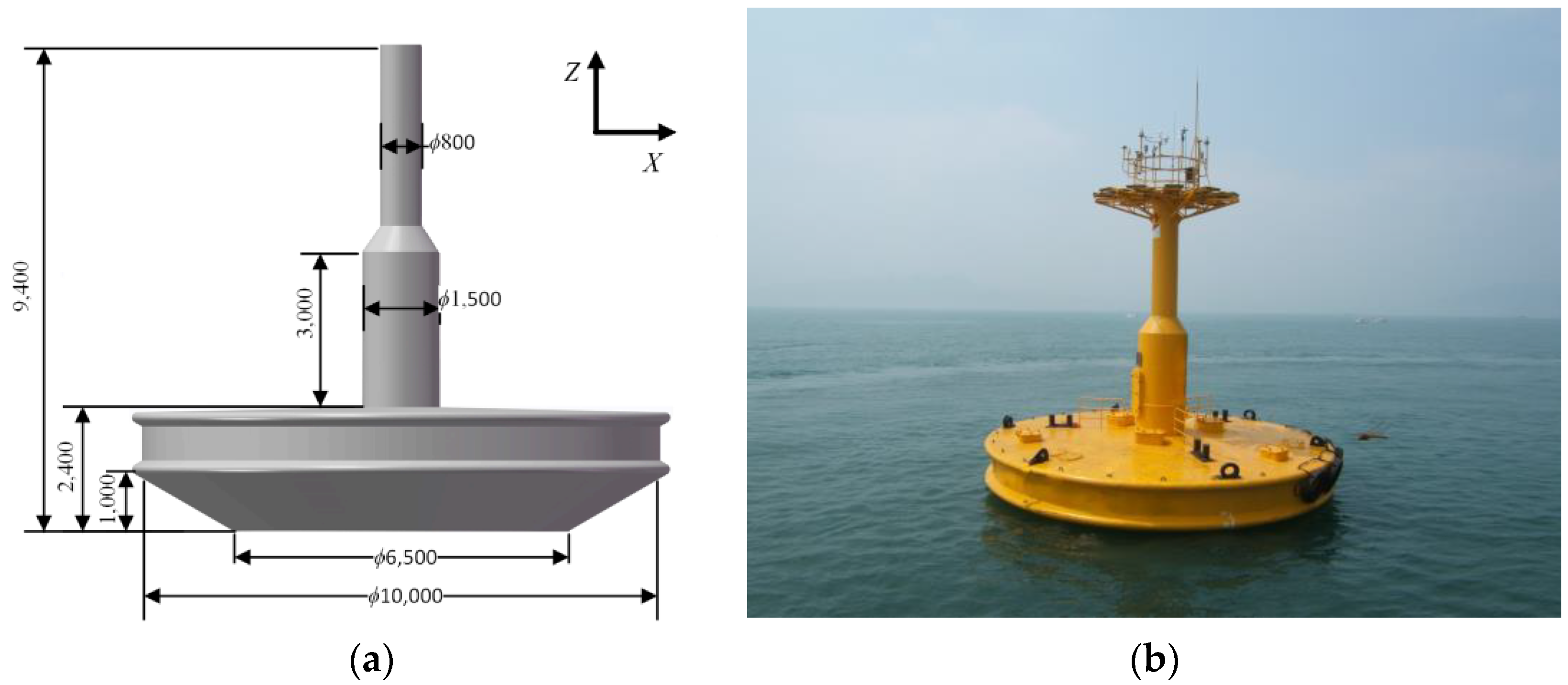
2.2. The Geometric Parameters of the Buoy

A large ocean-environment-monitoring buoy with an actual size of 10 m was used in this study. It had a conical base, a cylindrical middle section, and a monitoring platform at the top. Figure 1b shows the operational scenario in the field. To facilitate the study of the buoy’s hydrodynamic performance, a simplified model of the buoy was created, omitting some non-essential features above the water surface, as shown in Figure 1a. The mooring system of the buoy employed a single-point mooring, anchored in waters at a depth of 100 m. The fairlead hole was centered at the bottom of the buoy. An elastic catenary model was adopted for the anchor chain. Its dynamic response was entirely linear and did not consider the interaction with the seabed.

Table 1. Characteristics of the ocean buoy.

Models	Parameter	Value
Buoy	Mass (kg)	50,600
	Center of gravity (m)	(0, 0, 0.108)
	Draft (m)	0.950
	Moment of inertia, Ixx (kg∙m2)	361,000
	Moment of inertia, Iyy (kg∙m2)	361,000
	Moment of inertia, Izz (kg∙m2)	460,000
Mooring line	Diameter (m)	0.046
	Mass/unit length (kg/m)	48.400
	Location of the fairlead (m)	(0, 0, −1.150)
	The stiffness (kN/m)	3.000 × 107
	The length (m)	101.700

lists the basic structural parameters of the buoy system.

2.3. Test Cases in Marine Environment

The buoy has been installed for a long time in the South China Sea; thus, the conditions for the numerical simulations were primarily determined by the wave characteristics of this region [22]. To investigate the hydrodynamic performance of the buoy, two sets of wave conditions, with different strategies, were used in the numerical simulations. Different incident wave periods and wave steepnesses were considered, as shown in

Table 2. Variation in wave period test cases.

Test Cases	Wave Height H (m)	Wave Period T (s)	Wave Length L (m)
LC1	1.00	2.40	8.98
LC2	1.00	2.70	11.37
LC3	1.00	3.00	14.04
LC4	1.00	3.50	19.11
LC5	1.00	4.00	24.96
LC6	1.00	4.50	31.58
LC7	1.00	5.40	45.48
LC8	1.00	7.40	85.41

and

Table 3. Variation in wave steepness test cases.

Wave Parameter	LC9	LC10	LC11	LC12	LC13
H/L (−)	0.07	0.06	0.04	0.03	0.02
H (m)	1.40	1.20	0.80	0.60	0.40
T (s)	3.50	3.50	3.50	3.50	3.50
L (m)	19.11	19.11	19.11	19.11	19.11

. All incident waves were regular waves propagating along the positive x-axis.

3. Model Verification

This section describes the establishment of the numerical wave tank (NWT) and the verification of the numerical model, including the verification of the numerical wave and the convergence analysis of the mesh and time step.

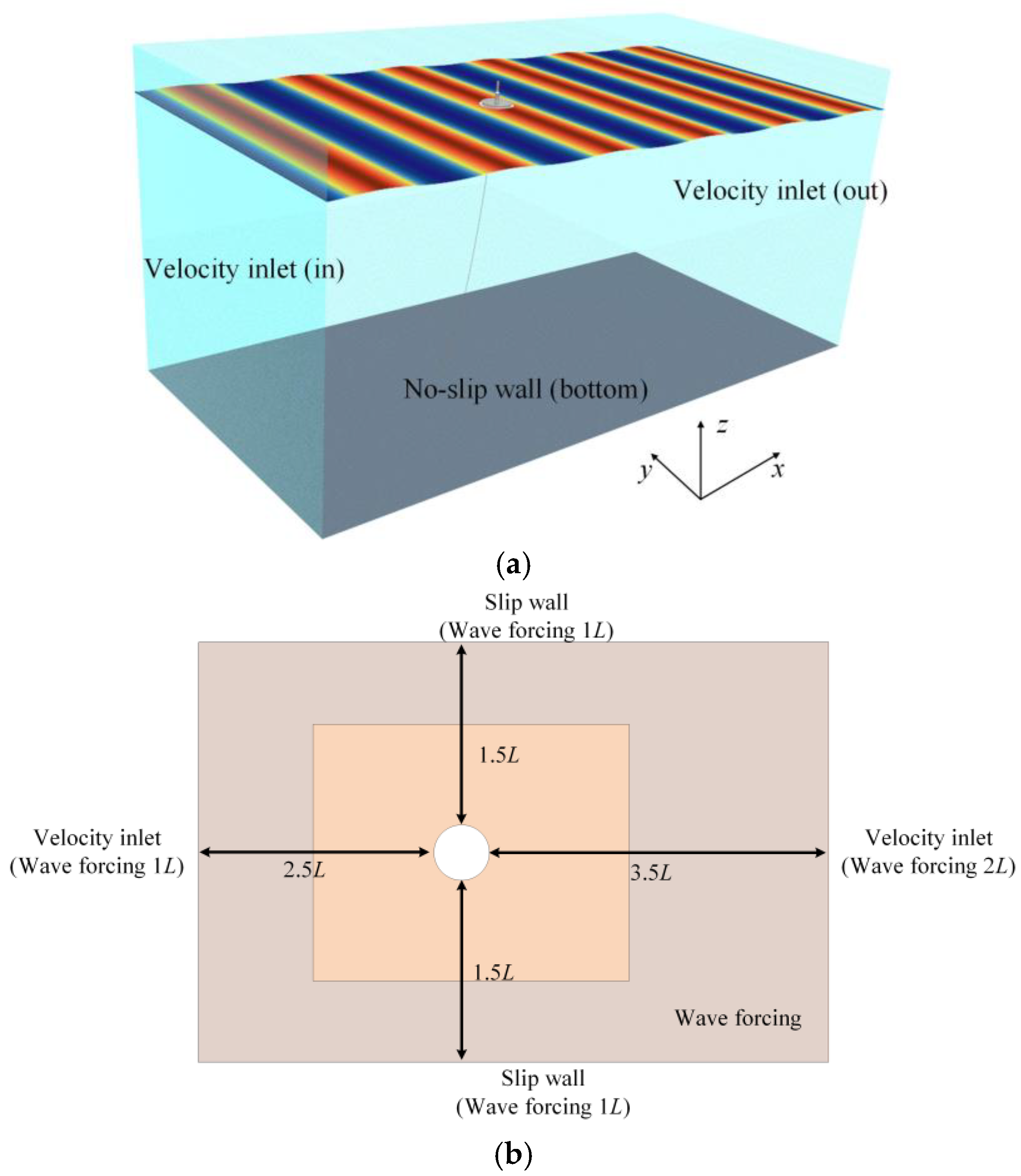
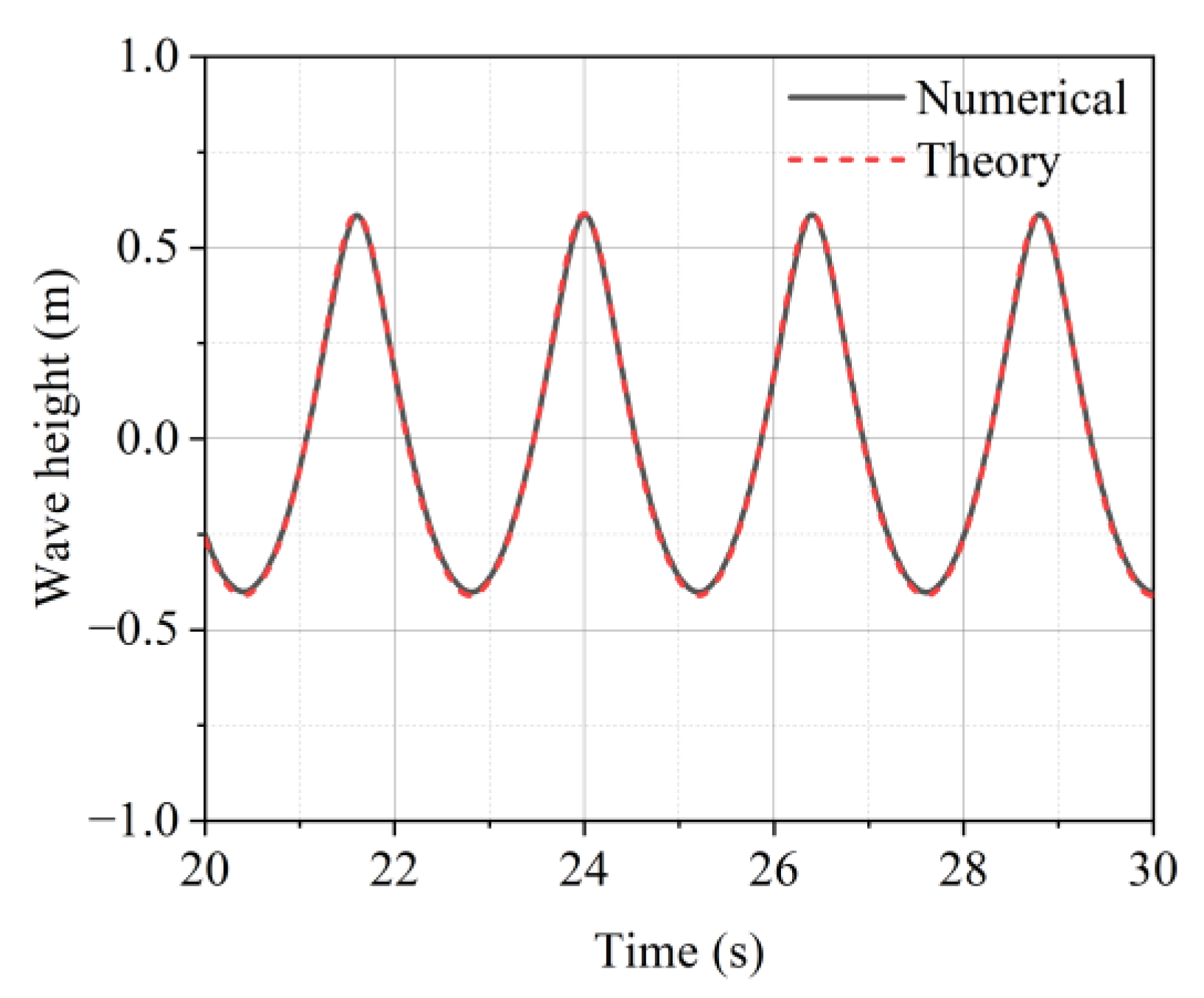
3.1. Numerical Wave Tank

The NWT was set as a rectangular cuboid, as shown in Figure 2, with a length of 6L (L being the incident wave wavelength) and a width of 3L. The left side of the tank served as the inlet boundary. Waves were generated via the boundary wave generation method. Waves propagated along the positive x-axis, and the origin location was the center of gravity of the buoy. The inlet and outlet boundaries were defined as velocity inlets, the side and bottom boundaries were specified as slip walls, and the top boundary was defined as a pressure outlet. The buoy was positioned 2.5L away from the inlet. Furthermore, the wave forcing approach was used at the boundary of the NWT to eliminate wave reflection.

Table 4. The physical properties of the fluids used in the simulations.

Type	Dynamic Viscosity (Pa–s)	Density (kg/m3)
Water	1.003 × 10−2	1.025 × 103
Air	1.855 × 10−5	1.205

lists the physical properties of the fluids used in the simulations.

A fifth-order wave was modelled with a fifth-order approximation to the Stokes theory of waves. This wave, which better captures nonlinear wave phenomena, more closely resembles a real wave than a wave that is generated by the first-order method. These related theories stem from the work by Fenton [23], as shown in Equation (8).

$$\begin{array}{l}\varphi ={\displaystyle \frac{c}{k_5}}{\displaystyle \sum _{n=1}^5{{\varphi }^{\prime }}_n}[chn{k}_5(z+d)]\sin n\theta \\ \eta ={\displaystyle \frac{1}{k_5}}{\displaystyle \sum _{n=1}^5{{\eta }^{\prime }}_n}\cos n\theta \\ u=c{\displaystyle \sum _{n=1}^{5}n{{\varphi }^{\prime }}_n}[chn{k}_5(z+d)]\cos n\theta \\ c=\sqrt{{\displaystyle \frac{gth{k}_{5}d(1+{\gamma }^2{C}_1+{\gamma }^4{C}_2)}{k_5}}}\end{array}$$

(8)

where ϕ is the velocity potential, η is the wave amplitude, u represents the horizontal phase velocity, and k₅ is the wave number.

At the inlet boundary, fifth-order Stokes waves was generated via a boundary wave-making method, which better captured nonlinear wave phenomena and more accurately reflected real ocean conditions. To improve the accuracy of the wave simulation, a refined mesh region was set near the free surface. A wave-forcing technique was applied at the surrounding boundaries to prevent wave reflection, with the length typically ranging from one to two times the incident wave wavelength. To assess the accuracy of the numerical wave, a wave gauge was placed at the buoy location to monitor the wave heights during empty-tank wave generation. Figure 3 presents a comparison of the time history between the numerical and theoretical wave heights. This shows a high degree of agreement, indicating that the numerical wave was both accurate and stable.

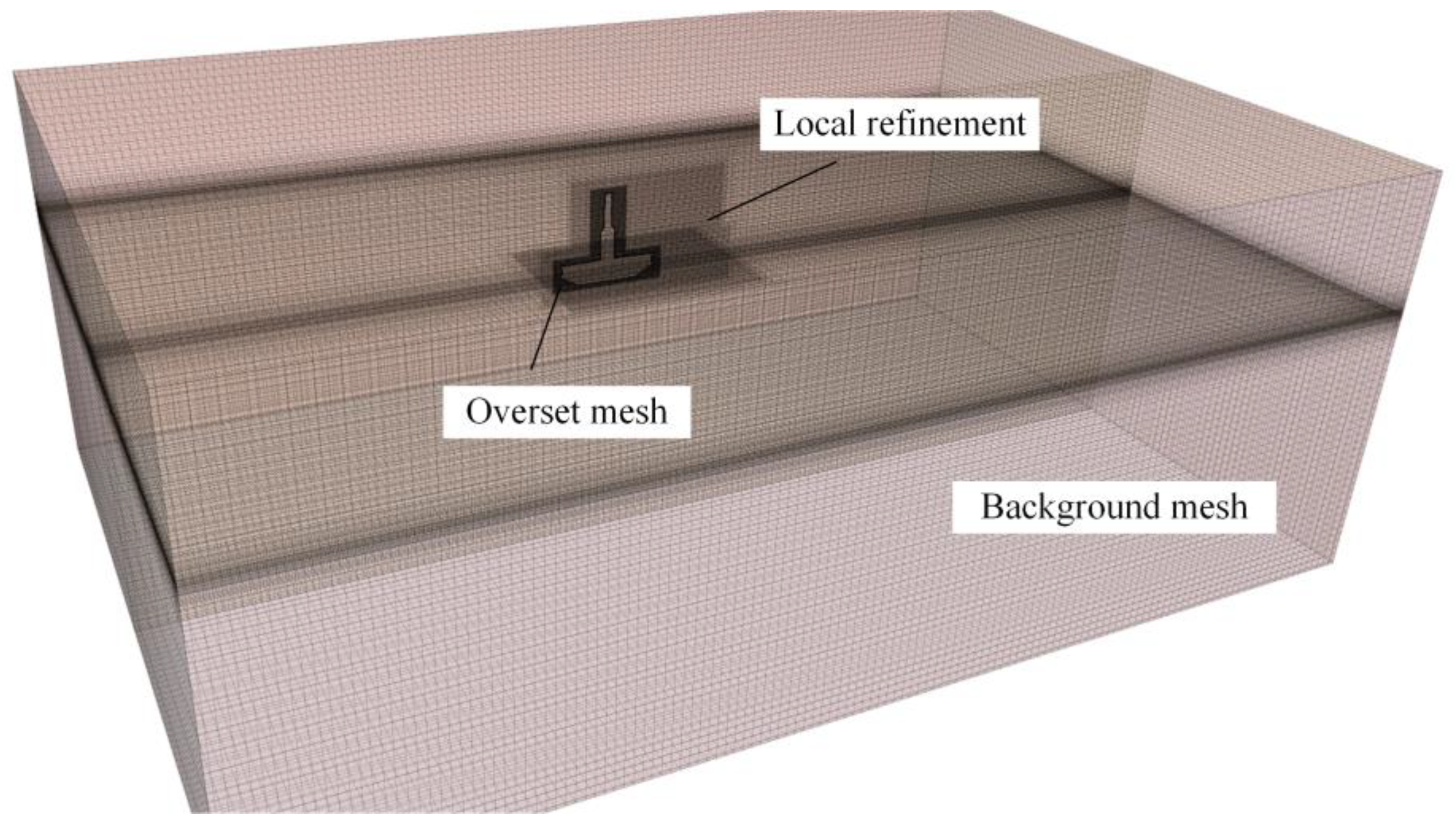
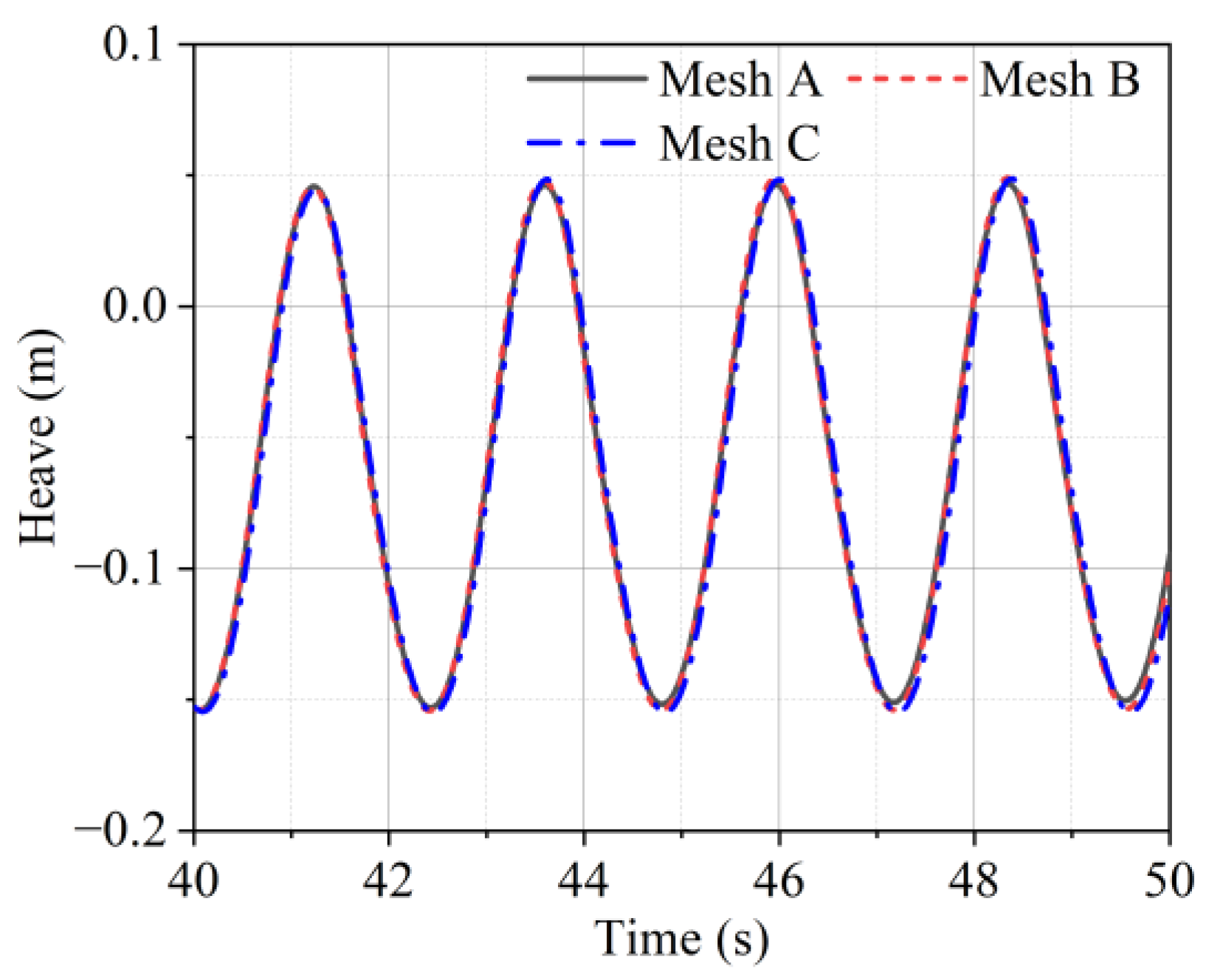
3.2. Mesh Convergence

Figure 4 shows the grid division of the tank. The entire mesh region consisted of a background mesh and an overset mesh. To ensure the effectiveness of the overset mesh, the overset region was maintained at a minimum of four grid layers away from the surface. Linear interpolation was employed to couple the solution between the overset region and the background region. These two grids overlapped in an arbitrary manner to address buoy motion. An overset mesh interface coupled the overset region with the background region. Notably, the cell sizes in the overlapping region between the overset and background grids should be similar during mesh generation. To maintain numerical accuracy, the background grid was refined in the motion area.

Before the case calculations, a grid convergence analysis of the NWT was conducted to systematically verify the effects of different grid sizes on the computational accuracy. A typical regular wave condition with a wave height of H = 1 m and a period of T = 2.4 s was selected for the simulation.

Table 5. Mesh size.

Mesh	Base Size (m)	L/∆x	H/∆z	Total Number
A	0.160	63	12	2,158,186
B	0.113	89	17	5,674,459
C	0.080	125	25	14,324,774

presents the three grid scales used in this study, with a constant refinement ratio of $\sqrt{2}$ between grid sizes. ∆x and ∆z represent the smallest grid cell sizes in the x and z directions, respectively. ∆x was 50% of the base size, whereas ∆z was 25% of the base size.

The center of gravity of the buoy was selected as the measuring point, and the heave responses of the buoy were selected as the variables to conduct the procedure. Figure 5 shows the time history of the buoy heave responses under different grid resolutions. The relative differences in the response amplitudes were 2.52% and 0.2%, respectively. Considering both the simulation accuracy and computational cost, mesh B was selected for use in subsequent simulations.

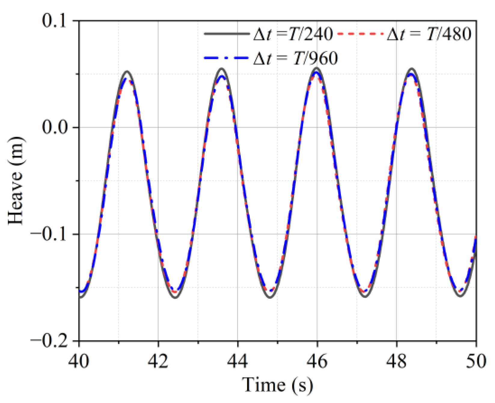
3.3. Time-Step Convergence

Next, a time-step convergence analysis was performed under the same incident wave conditions based on mesh B. Three simulations were executed with different time steps: ∆t = T/240 s, T/480 s, and T/960 s. The constant refinement ratio between time steps was set to 2. Figure 6 displays the time history of the heave motion for the different time steps. A comparison of the motion amplitudes revealed numerical differences of 4.69% and 1.27% between ∆t = T/240 s and ∆t = T/480 s and ∆t = T/960 s, respectively. To balance numerical accuracy and computational cost, a time step of ∆t = T/480 s was selected for further calculations.

4. Results and Discussion

To investigate the hydrodynamic performance of the buoy, a series of numerical simulations were conducted. These included free decay tests and studies on the effects of different wave periods and wave heights on the motion response. Finally, the full-scale field data were used for verification. Notably, all motion responses were measured based on the basis of the center of gravity.

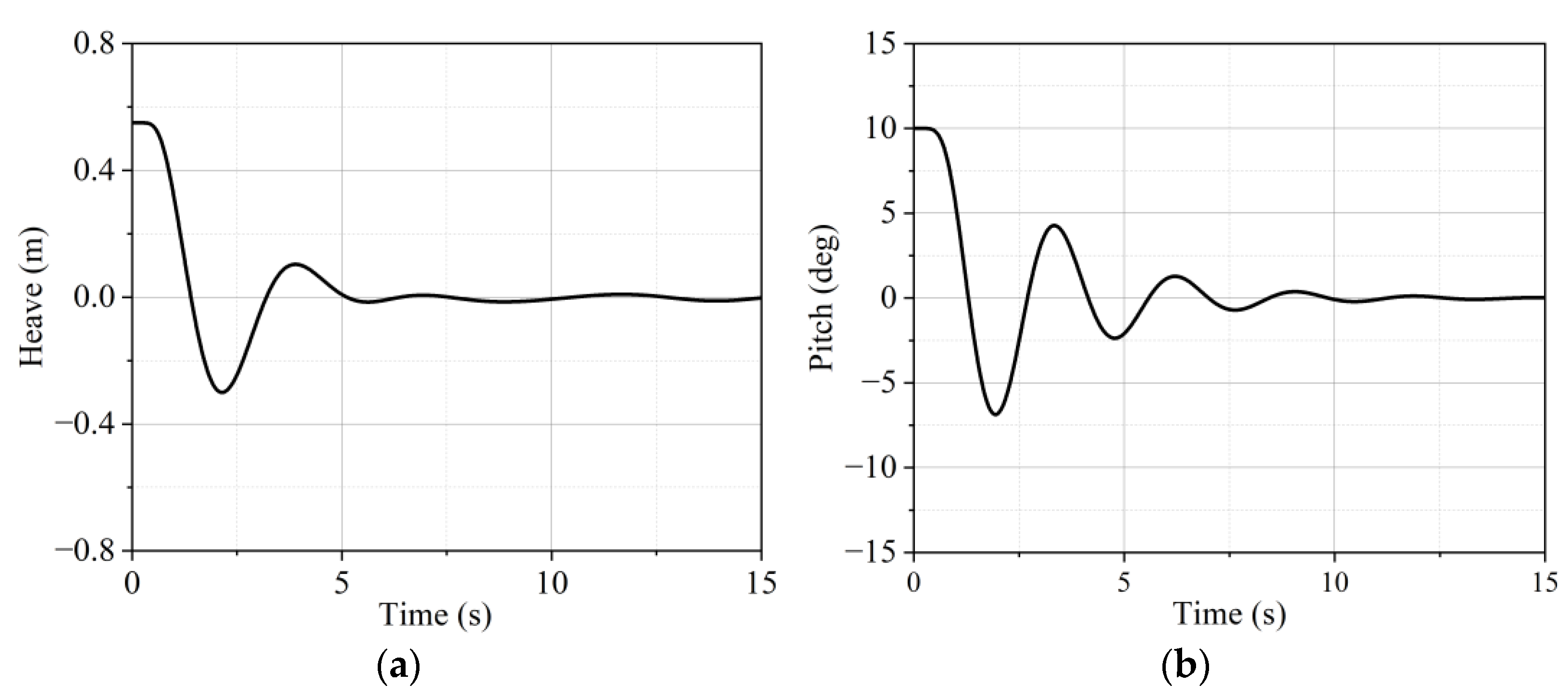
4.1. Free Decay Test

The natural period, which is determined by the inherent properties of the structure, is a critical factor influencing buoy motion. When the excitation period approaches the natural period, resonance occurs, which amplifies the buoy’s motion response. Therefore, a free decay test was first performed on the buoy with a mooring system. Owing to the single-point mooring configuration, the restoring force in the surge direction was relatively weak. Consequently, this study conducted free decay tests with only heave and pitch degrees of freedom.

Notably, each test was initiated by applying an initial displacement of only one degree of freedom under steady water conditions. The buoy, influenced by restoring forces, underwent periodic decay motions and gradually returned to equilibrium. By recording the buoy’s motion responses, the time history for each degree of freedom was obtained. Figure 7 shows the free decay time history of the buoy’s heave and pitch motions. The heave motion decayed very quickly because of the large damping effect of the buoy’s base, which acted like a large damping plate. To improve the accuracy of the natural period estimation, multiple free decay tests were performed by releasing the buoy from different heights. The natural period can be calculated by Equation (8). The natural period for heave was found to be 3.46 s, and for pitch, it was 2.84 s.

$$T={\displaystyle \frac{t_{i+k}-t_i}{k}}$$

(9)

where T represents the natural period, and t_i+k and t_i correspond to the times associated with the (i + k)^th and ith amplitude peaks, respectively.

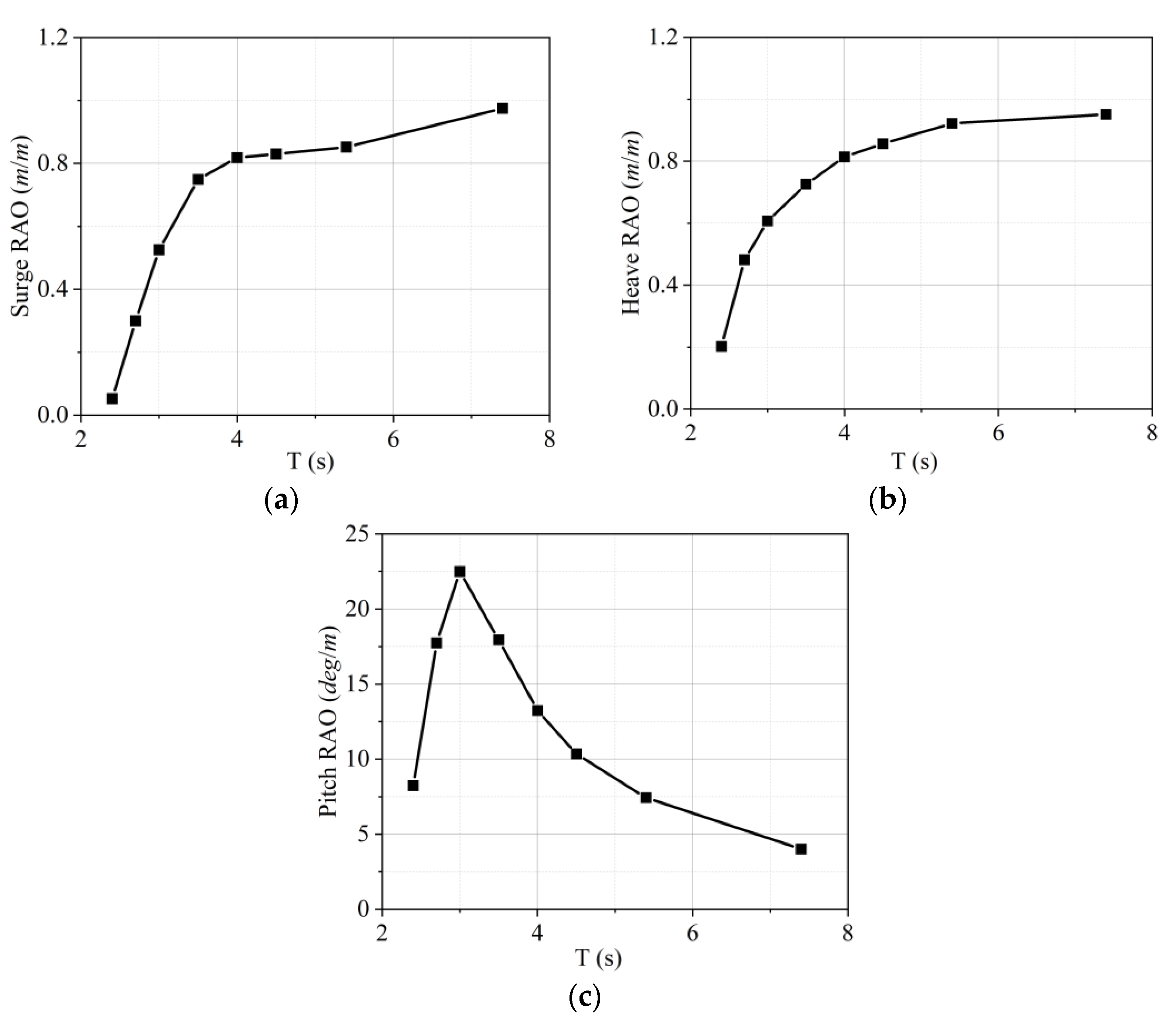
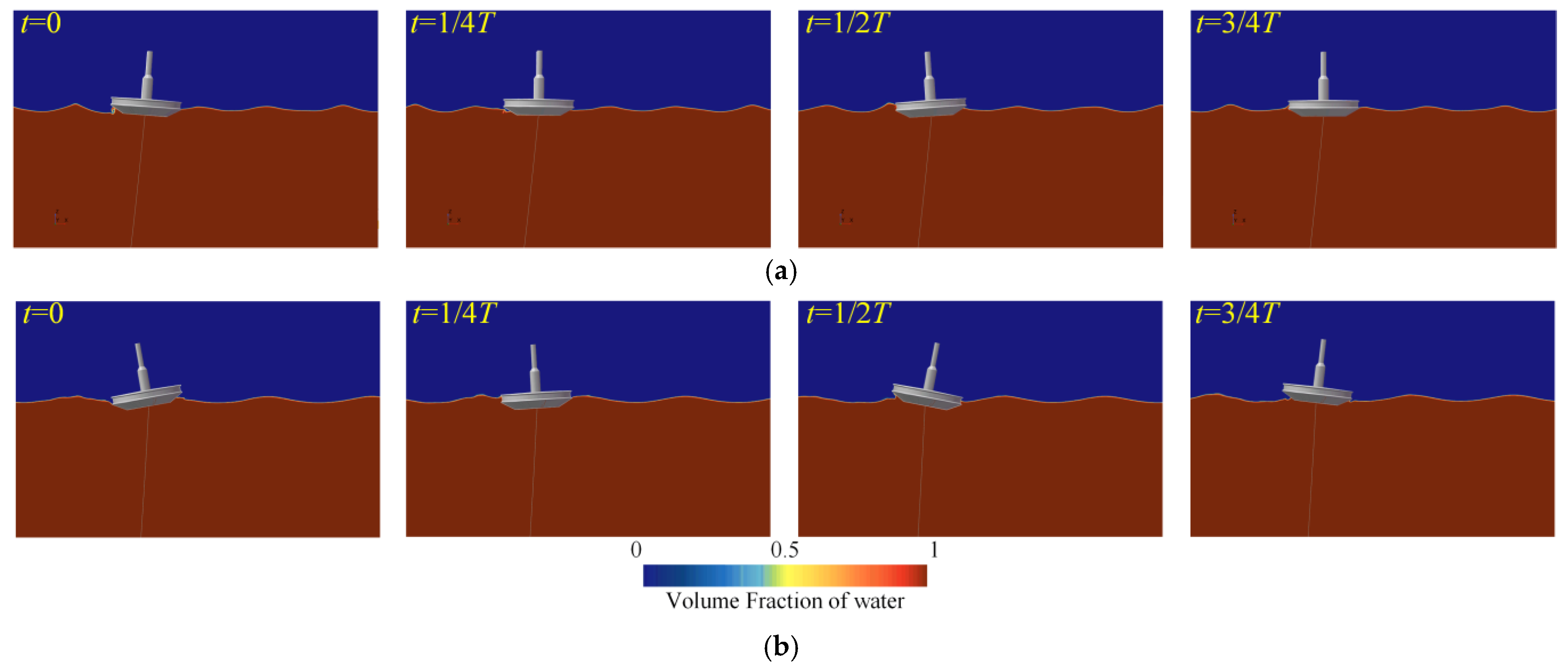
4.2. Effect of Wave Period

This subsection compares the motion responses of the buoy under different wave periods. All the conditions involved regular waves with a wave height of 1 m, as detailed in Table 2. Under the combined effects of regular waves and the mooring system, the buoy’s motion could stabilize after a period of development. The motion characteristics were analyzed by calculating the response amplitude operator (RAO). Figure 8 presents the motion responses of the buoy in three degrees of freedom: heave, surge, and pitch. The surge motion of the buoy increased with the wave period, which was influenced primarily by the horizontal wave forces and the restoring force of the mooring system. The mooring chain was not fully tensioned under all test cases. The heave motion also increased with the wave period, ultimately approaching the height of the incident waves. Notably, there was no significant resonance during the natural period of heave because of the large amount of radiation damping resulting from the bottom shape. The pitch motion first increased and then decreased as the wave period increased, reaching a maximum near the natural period of pitch. The buoy exhibited pronounced resonance under wave action.

Harmonic analysis via fast Fourier transform (FFT) was performed on the buoy’s motion response to study the nonlinear interaction between waves and structures. Figure 9 displays the frequency spectral patterns of the heave and pitch motions of the buoy under test cases LC1 and LC2. The buoy motion was influenced primarily by the first-order harmonic component of the waves, with higher-order harmonic components contributing relatively little. In LC1, the presence of third and fourth harmonics indicates that the buoy experienced nonlinear motion responses. However, as the wave period increased, the higher-order harmonic components gradually diminished. Figure 10 shows the changes in the free surface around the buoy over one wave period. It can be observed that the wave shape significantly changed on both the weather side and the lee side of the buoy, particularly under condition LC1, resulting in substantial wave slamming and wave run-up. Figure 11 shows the pressure nephogram at the bottom of the buoy within one wave period. It can be clearly found that the run-up and slamming occurred in the direction of the incident wave. These phenomena increased the wave impact forces on the buoy, thereby affecting the stability of the system.

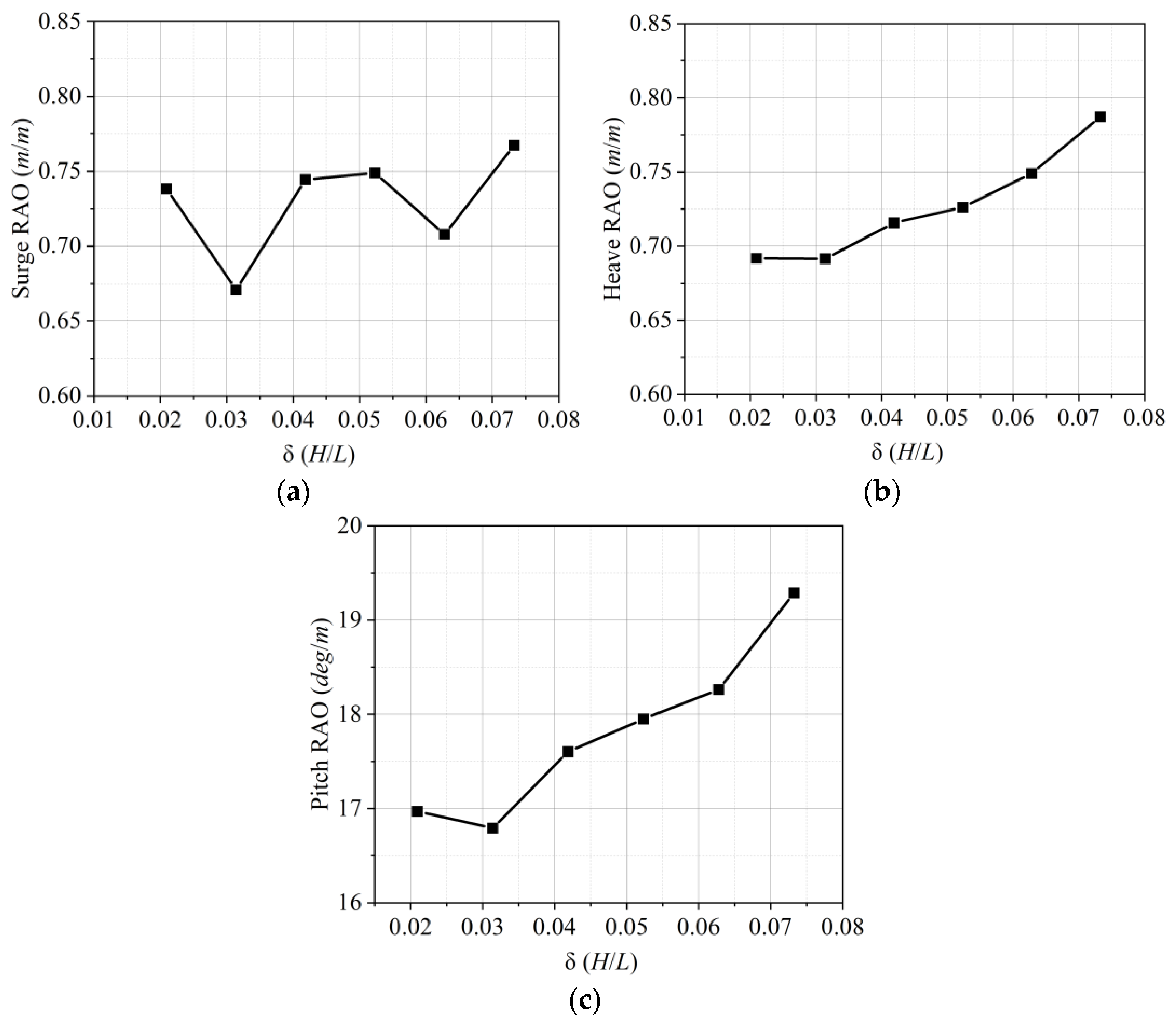
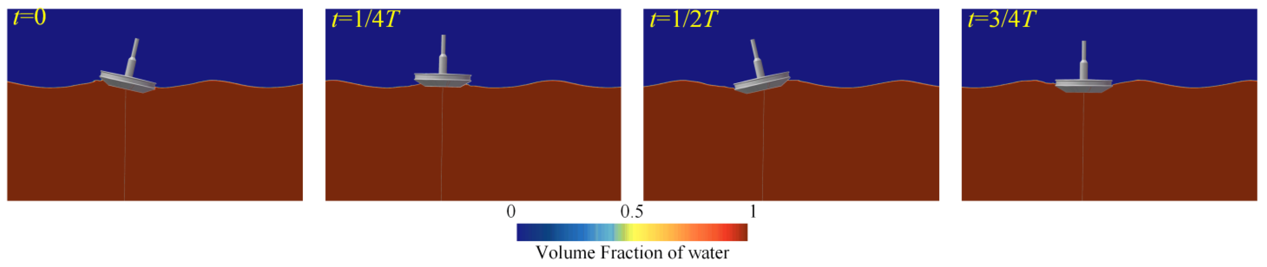
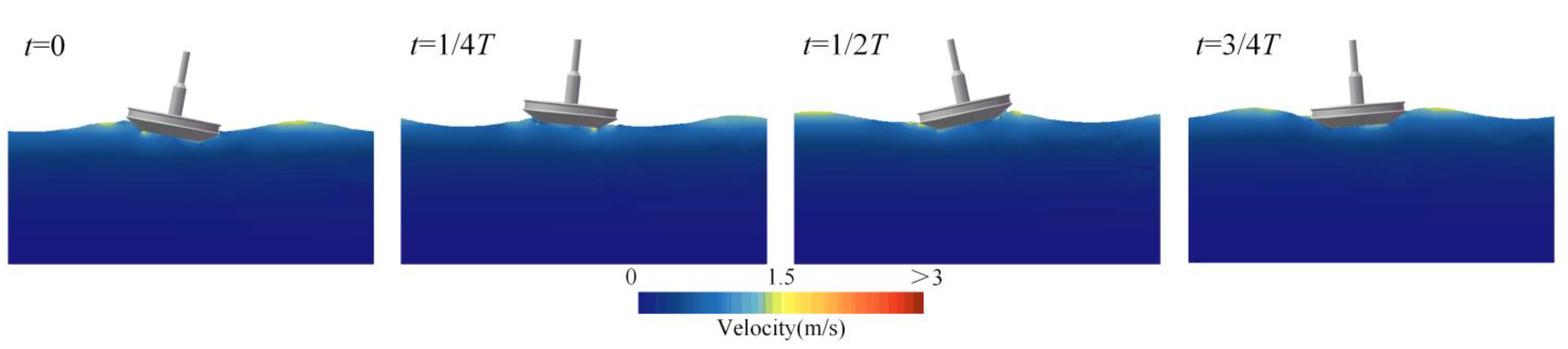
4.3. Effect of Wave Steepness

This section investigates the motion responses of the buoy under varying wave steepness values, ranging from 0.02 to 0.07, with the specific test conditions detailed in Table 3. Figure 12 presents the variations in the RAO of the buoy motion obtained in the NWT. The results indicate that different degrees of freedom exhibited varying sensitivities to the wave steepness. Notably, the impact of the wave steepness on the surge motion was relatively low. During the simulations, while increasing the wave steepness led to greater amplitudes of surge motion, the slow drift distance of the buoy also increased. This resulted in a tightening of the mooring lines, which increased the restoring forces provided by the mooring system. For heave and pitch motions, the RAOs increased by 13.78% and 13.65%, respectively (from LC13 to LC9), as the wave steepness increased. This was attributed primarily to the enhanced nonlinear wave–structure interactions resulting from the increased wave steepness.

To further analyze the nonlinear interaction between waves and the structure, harmonic analysis via FFT was conducted on the heave and pitch motions of the buoy. Figure 13 shows the frequency spectral patterns of the motion responses under test conditions LC9 and LC10, with the vertical axis representing the non-dimensionalized motion response amplitude η. With increasing wave steepness, the second-order components of the buoy motion progressively increased, indicating an increase in the nonlinear effects between the waves and the structure. In contrast, the contributions of the first-order harmonic amplitude showed opposing behaviors for the heave and pitch motions. As the wave steepness increased, the contribution of the first-order component to the pitch motion gradually decreased. Figure 14 and Figure 15 show the free surface and velocity nephograms around the buoy under large-amplitude wave conditions. It is evident that the buoy’s motion and wave motion clearly exhibited a strong coupling effect, with closely aligned phases. As the amplitude of the wave motion increased, the wave forces acting on the buoy also increased, resulting in more pronounced changes in the waterline. However, due to the faster fluid velocities and larger wave amplitudes, the buoy’s influence on the wave surface and velocity field decreased. Figure 16 shows the vorticity nephogram around the buoy during one wave period and shows the dramatic changes in the interface between the buoy and the wave.

4.4. Validation with Full-Scale Field Data

To investigate the motion response of the buoy in a real ocean environment, full-scale field data were used to validate the numerical methods. The prototype buoy was deployed in the South China Sea. The measurement instruments installed on the buoy recorded the water surface elevation and motion responses on 22 August 2017. A 600 s segment of wave data was selected for analysis, as shown in Figure 17, during which components below 0.1 Hz were excluded because they were deemed related to the slow drift of the measuring buoy. Power spectral density analysis revealed that the measured waves could be approximated by the JONSWAP spectrum, with a peak period of 3.23 s and a significant wave height of 0.75 m. Figure 18 shows the power spectral density of the measured water surface elevation and its comparison with the simulation spectrum. The results indicate that the simulated JONSWAP spectrum and the measured waves exhibited good and consistent statistical characteristics. Furthermore, it was assumed that the wave direction remained constant throughout the duration of the measurement.

The pitch motion of a buoy has the greatest impact on the accuracy of the wind speed measurement sensors. Therefore, this analysis focused exclusively on the pitch motion. Owing to discrepancies between the measured and simulated input wave time histories, frequency domain analysis was performed via FFT. Figure 19 shows the good consistency between the measured and simulated values, both of which exhibited a spectral peak corresponding to the buoy’s natural pitch frequency. This indicates that the pitch motion response of the buoy was influenced by resonance. To ensure the accuracy of the sensors, the natural frequency of the buoy should avoid wave frequencies present in the deployment area. Snapshots of the flow field revealed significant changes in the free surface around the buoy, as shown in Figure 20. Under irregular wave loads, the probability of wave run-up increased markedly, often accompanied by substantial motion responses of the buoy.

5. Conclusions

This study investigated the motion of large ocean buoys under various sea conditions by establishing a numerical wave tank to assess buoy performance and stability. First, a three-dimensional numerical wave tank for handling wave–structure interactions was developed via an overset mesh method and the volume of fluid method, and mesh and time-step convergence analyses were conducted. Free decay tests were subsequently conducted to determine the buoy’s natural frequencies. This study then focused on the buoy’s motion responses under different wave conditions, particularly terms of the degrees of freedom of surge, heave, and pitch. The following conclusions were drawn from the analysis:

1.

In the free decay tests, the unique bottom shape of the buoy acted as a damping plate, generating substantial radiation damping, which led to a rapid decay in heave motion. The natural periods for heave and pitch were measured to be 3.46 s and 2.84 s, respectively.

2.

The response characteristics of the buoy’s motion under different sea conditions were analyzed via the response amplitude operator and frequency spectral patterns. The heave response approached the amplitude of the waves as the wave period increased. The maximum RAO for pitch motion was close to the buoy’s natural frequency. As the wave steepness increased, the nonlinearity of the waves intensified, resulting in an increased motion response of the buoy. This made the nonlinear interactions between the waves and the structure more pronounced.

3.

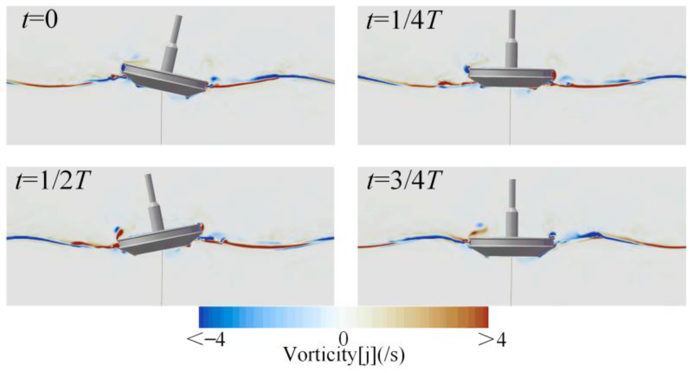
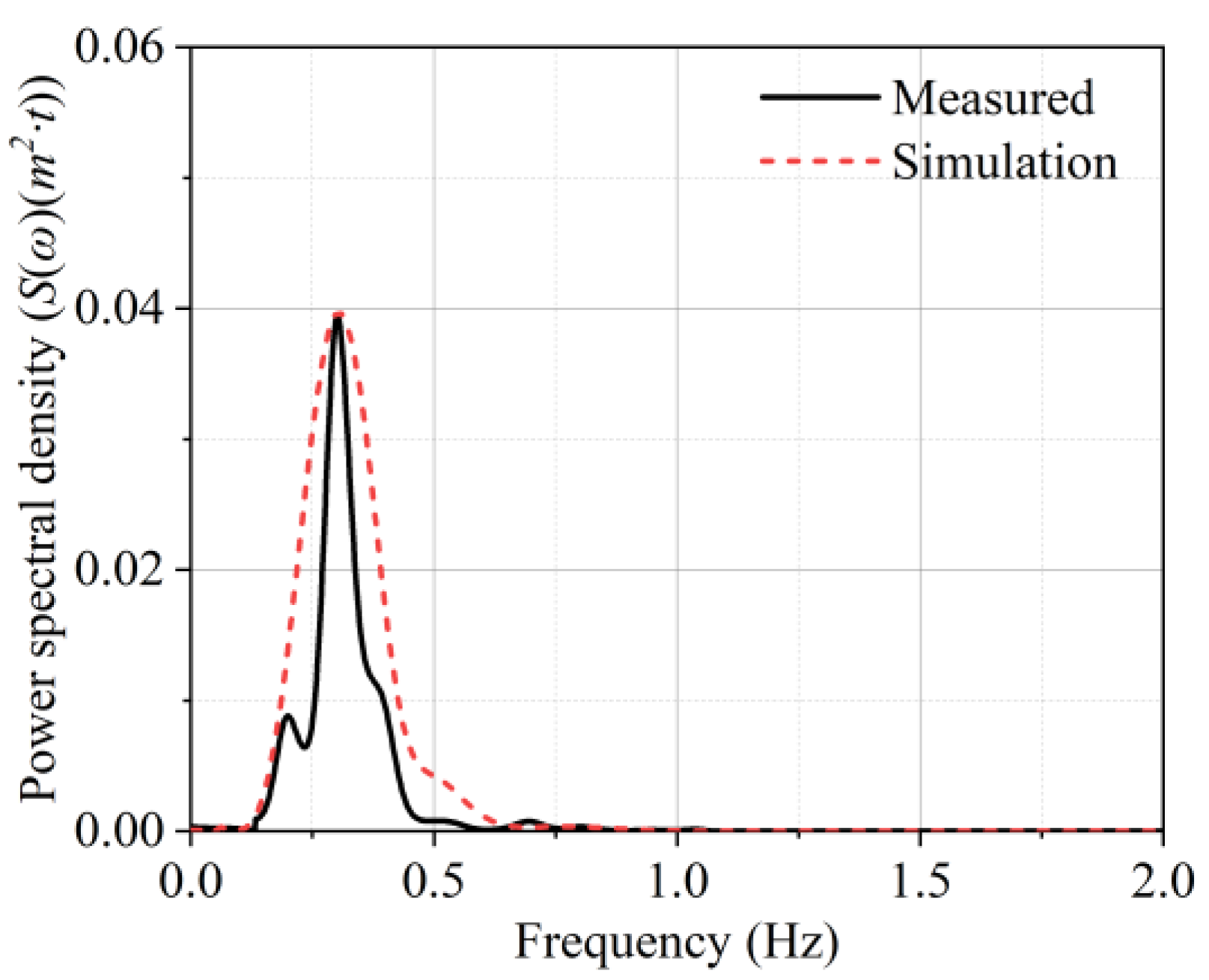
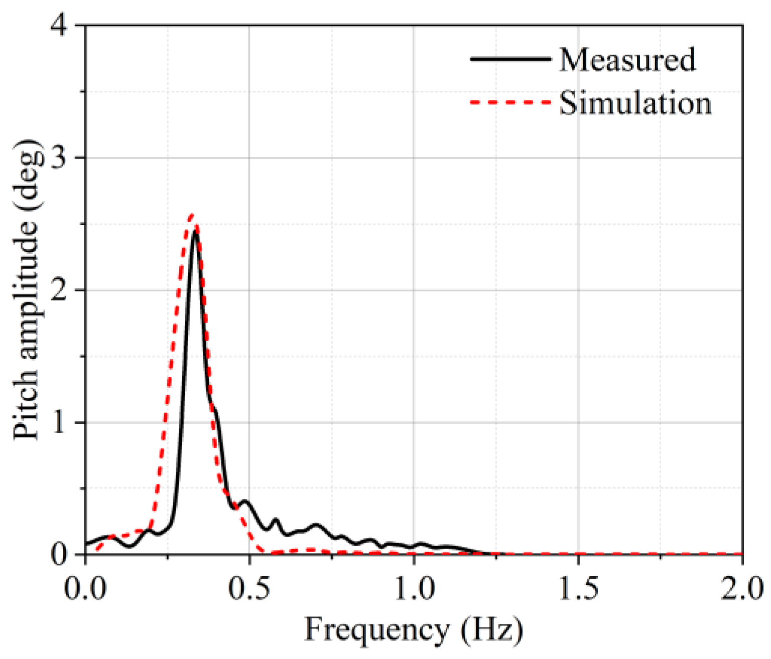
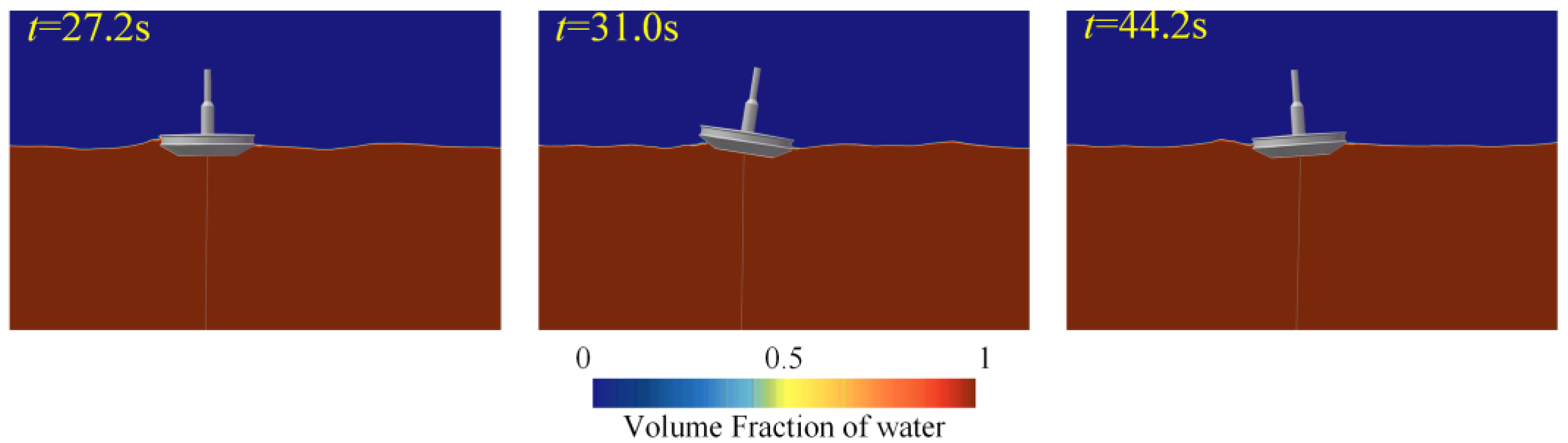
The numerical simulations of the dynamic responses under irregular waves were conducted via full-scale field time series data and compared with field data. A comparison between the wave surface and the buoy pitch motion revealed a fairly good agreement.

Because other degrees of freedom data are not available at present, the validation with full-scale field data was limited to the pitch motion. Future work will consider incorporating a broader range of degrees of freedom for a more comprehensive validation. Furthermore, considering the practical engineering significance of buoys, we plan to establish a calibration relationship between the buoy’s motion response and measured environmental data such as wave elevation and wind speed to more accurately estimate environmental data.

References

1. Wang, L.; Li, H.; Jiang, J. A High-Efficiency Wave-Powered Marine Observation Buoy: Design, Analysis, and Experimental Tests. Energy Convers. Manag. 2022, 270, 116154. [Google Scholar] [CrossRef]
2. Wang, J.; Wang, Z.; Wang, Y.; Liu, S.; Li, Y. Current Situation and Trend of Marine Data Buoy and Monitoring Network Technology of China. Acta Oceanol. Sin. 2016, 35, 1–10. [Google Scholar] [CrossRef]
3. Lin, M.; Yang, C. Ocean Observation Technologies: A Review. Chin. J. Mech. Eng. 2020, 33, 32. [Google Scholar] [CrossRef]
4. Draycott, S.; Pillai, A.C.; Gabl, R.; Stansby, P.K.; Davey, T. An Experimental Assessment of the Effect of Current on Wave Buoy Measurements. Coast. Eng. 2022, 174, 104114. [Google Scholar] [CrossRef]
5. Li, Y.; Yang, F.; Li, S.; Tang, X.; Sun, X.; Qi, S.; Gao, Z. Influence of Six-Degree-of-Freedom Motion of a Large Marine Data Buoy on Wind Speed Monitoring Accuracy. J. Mar. Sci. Eng. 2023, 11, 1985. [Google Scholar] [CrossRef]
6. Amaechi, C.V.; Wang, F.; Ye, J. Experimental Study on Motion Characterisation of CALM Buoy Hose System under Water Waves. J. Mar. Sci. Eng. 2022, 10, 204. [Google Scholar] [CrossRef]
7. Radhakrishnan, S.; Datla, R.; Hires, R.I. Theoretical and Experimental Analysis of Tethered Buoy Instability in Gravity Waves. Ocean Eng. 2007, 34, 261–274. [Google Scholar] [CrossRef]
8. Liu, W.; Wang, B.-F.; Zhang, J.; Dong, Y. A Numerical Analysis of Wave Type and Steepness Effects on Cylindrical Buoy Dynamic Characteristics. Ocean Eng. 2024, 311, 118923. [Google Scholar] [CrossRef]
9. Li, H.; Xu, C.; Tian, Y.; Qu, F.; Chen, J.; Sun, K.; Leng, J.; Wei, Y. The Design of a Novel Small Waterplane Area Pillar Buoy Based on Rolling Analysis. Ocean Eng. 2019, 184, 289–298. [Google Scholar] [CrossRef]
10. Hu, J.; Zhu, L.; Liu, S. Analysis and Optimization on the Flow Ability of Wave Buoy Based on AQWA. IOP Conf. Ser. Earth Environ. Sci. 2018, 171, 012004. [Google Scholar] [CrossRef]
11. Zheng, H.; Chen, Y.; Liu, Q.; Zhang, Z.; Li, Y.; Li, M. Theoretical and Numerical Analysis of Ocean Buoy Stability Using Simplified Stability Parameters. J. Mar. Sci. Eng. 2024, 12, 966. [Google Scholar] [CrossRef]
12. Jeong, S.-M.; Son, B.-H.; Lee, C.-Y. Estimation of the Motion Performance of a Light Buoy Adopting Ecofriendly and Lightweight Materials in Waves. J. Mar. Sci. Eng. 2020, 8, 139. [Google Scholar] [CrossRef]
13. Amaechi, C.V.; Wang, F.; Ye, J. Numerical Studies on CALM Buoy Motion Responses and the Effect of Buoy Geometry Cum Skirt Dimensions with Its Hydrodynamic Waves-Current Interactions. Ocean Eng. 2022, 244, 110378. [Google Scholar] [CrossRef]
14. Li, X.; Bian, Y. Modeling and Prediction for the Buoy Motion Characteristics. Ocean Eng. 2021, 239, 109880. [Google Scholar] [CrossRef]
15. Deng, H.; Li, X.; Zhu, J.; Liu, Y. Transfer Learning for Modeling and Prediction of Marine Buoy Motion Characteristics. Ocean Eng. 2022, 266, 113158. [Google Scholar] [CrossRef]
16. Jin, Y.; Xie, K.; Liu, G.; Peng, Y.; Wan, B. Nonlinear Dynamics Modeling and Analysis of a Marine Buoy Single-Point Mooring System. Ocean Eng. 2022, 262, 112031. [Google Scholar] [CrossRef]
17. Ma, C.; Iijima, K.; Nihei, Y.; Fujikubo, M. Theoretical, Experimental and Numerical Investigations into Nonlinear Motion of a Tethered-Buoy System. J. Mar. Sci. Technol. 2016, 21, 396–415. [Google Scholar] [CrossRef]
18. Li, X.; Chen, Y.; Mao, L.; Xia, H. Numerical Investigation of Hydrodynamic Performance of a Light Buoy With Different Mooring Configurations in Regular Waves. J. Offshore Mech. Arct. Eng. 2022, 144, 021904. [Google Scholar] [CrossRef]
19. Zhu, X.; Yoo, W.S. Dynamic Analysis of a Floating Spherical Buoy Fastened by Mooring Cables. Ocean Eng. 2016, 121, 462–471. [Google Scholar] [CrossRef]
20. Chen, S.; Zhang, J.; Liu, S.; Tao, B.; Wu, Y.; Wan, X.; Xu, Y.; Song, M.; Yan, X.; Yang, X.; et al. Structure Design and Implementation of a High Stability Semi-Submersible Optical Buoy for Marine Environment Observation. Ocean Eng. 2023, 290, 116217. [Google Scholar] [CrossRef]
21. Amaechi, C.V.; Wang, F.; Ye, J. Understanding the Fluid–Structure Interaction from Wave Diffraction Forces on CALM Buoys: Numerical and Analytical Solutions. Ships Offshore Struct. 2022, 17, 2545–2573. [Google Scholar] [CrossRef]
22. Luan, Z.; Chen, B.; He, G.; Cui, T.; Ghassemi, H.; Zhang, Z.; Liu, C. Research on Wavestar-Like Wave Energy Converter Arrays with a Truss-Type Octagonal Floating Platform in the South China Sea. Energy 2024, 313, 134070. [Google Scholar] [CrossRef]
23. Fenton, J.D. A Fifth-Order Stokes Theory for Steady Waves. J. Waterw. Port Coast. Ocean Eng. 1985, 111, 216–234. [Google Scholar] [CrossRef]
Figure 1. The ocean buoy model and its geometric dimensions: (a) simplified buoy model; (b) the prototype of the ocean buoy.
Jmse 13 00822 g001
Figure 2. Graphic visualization of the NWT: (a) boundary condition; (b) geometric dimension.
Jmse 13 00822 g002
Figure 3. Comparison of the time history of wave elevation between the numerical and theoretical results.
Jmse 13 00822 g003
Figure 4. Mesh partition and refinement.
Jmse 13 00822 g004
Figure 5. Time history of heave responses at different mesh resolutions.
Jmse 13 00822 g005
Figure 6. Time history of heave responses at different time steps.
Jmse 13 00822 g006
Figure 7. Time history of the free decay test: (a) the heave motion; (b) the pitch motion.
Jmse 13 00822 g007
Figure 8. The RAO of motion response: (a) the surge motion; (b) the heave motion; (c) the pitch motion.
Jmse 13 00822 g008
Figure 9. The FFT frequency spectral patterns of the motion response: (a) the heave motion under LC1; (b) the pitch motion under LC1; (c) the heave motion under LC2; (d) the pitch motion under LC2.
Jmse 13 00822 g009
Figure 10. The variation in the free surface around the buoy within one wave period: (a) LC1; (b) LC2.
Jmse 13 00822 g010
Figure 11. Pressure nephogram at the bottom of the buoy within one wave period in LC1.
Jmse 13 00822 g011
Figure 12. The RAO of the motion response: (a) the surge motion; (b) the heave motion; (c) the pitch motion.
Jmse 13 00822 g012
Figure 13. The FFT frequency spectral patterns of the motion response: (a) the heave motion; (b) the pitch motion.
Jmse 13 00822 g013
Figure 14. Wave surface contours around the buoy during one wave period in LC9.
Jmse 13 00822 g014
Figure 15. Velocity vector nephogram around the buoy during one wave period in LC9.
Jmse 13 00822 g015
Figure 16. Vorticity nephogram around the buoy during one wave period in LC9.
Jmse 13 00822 g016
Figure 17. The time history of wave height measured in the field.
Jmse 13 00822 g017
Figure 18. The comparison of the power spectral density.
Jmse 13 00822 g018
Figure 19. The FFT frequency spectral patterns of pitch motion.
Jmse 13 00822 g019
Figure 20. Flow field snapshot of free surface around the buoy.
Jmse 13 00822 g020