A Novel Swin-Transformer with Multi-Source Information Fusion for Online Cross-Domain Bearing RUL Prediction

Abstract

Accurate remaining useful life (RUL) prediction of rolling bearings plays a critical role in predictive maintenance. However, existing methods face challenges in extracting and fusing multi-source spatiotemporal features, addressing distribution differences between intra-domain and inter-domain features, and balancing global-local feature attention. To overcome these limitations, this paper proposes an online cross-domain RUL prediction method based on a swin-transformer with multi-source information fusion. The method uses a Bidirectional Long Short-Term Memory (Bi-LSTM) network to capture temporal features, which are transformed into 2D images using Gramian Angular Fields (GAF) for spatial feature extraction by a 2D Convolutional Neural Network (CNN). A self-attention mechanism further integrates multi-source features, while an adversarial Multi-Kernel Maximum Mean Discrepancy (MK-MMD) combined with a relational network mitigates feature distribution differences across domains. Additionally, an offline-online swin-transformer with a dynamic weight updating strategy enhances cross-domain feature learning. Experimental results demonstrate that the proposed method significantly reduces Root Mean Square Error (RMSE) and Mean Absolute Error (MAE), outperforming public methods in prediction accuracy and robustness.

1. Introduction

Rolling bearings are widely used in wind turbines, machine tools, marine engines, and other rotating equipment. Bearing failure can lead to production stagnation, equipment damage, or even major accidents. Therefore, developing a rolling bearing Remaining Useful Life (RUL) prediction model is crucial for maintenance, production efficiency, and equipment safety [1]. Feature extraction is a critical part of building an accurate rolling bearing RUL prediction model. Current research primarily focuses on extracting deep features from single-source bearings. However, extracting spatial and temporal features from multi-source online bearings presents several challenges. These challenges involve balancing feature information, reducing domain differences, and improving RUL prediction accuracy. These difficulties arise from the limited offline sample data, inefficient use of online datasets, and differences in feature distributions between multi-source and target domains. Consequently, the accuracy of RUL prediction models is low. To address these challenges, this paper conducts research aimed at enhancing the accuracy and reliability of RUL predictions.

Recent studies have proposed various feature extraction methods for rolling bearings, but they share common limitations. Siahpour et al. [2] and Zou et al. [3] developed stacked CNNs and convolutional autoencoders, respectively, but both either ignored essential features or lost useful bearing information. Pan et al. [4] combined CNN with self-attention mechanisms but overlooked fine-grained spatial details. Ren et al. [5] combined deep autoencoders with Deep Neural Networks to improve model efficiency. In contrast, Huang et al. [6] focused on time series features without addressing spatial feature extraction. Li et al. [7] and Miao et al. [8] introduced autoencoder-based CNN and adaptive CNN but struggled with spatiotemporal sequence information and deep feature extraction. Similarly, Zhuang et al. [9] and Berghout et al. [10] emphasized temporal features but neglected spatial series information. Mao et al. [11] improved temporal feature extraction but at the cost of increased model complexity and ignored spatial features. Although these methods excel at extracting local or global features, they fail to fuse spatiotemporal relationships effectively. In contrast, the proposed method overcomes these limitations by comprehensively integrating spatial and temporal features, enabling more accurate and robust extraction for rolling bearings.

Feature extraction methods are widely used in transfer learning frameworks for rolling bearing RUL prediction. However, challenges such as intra-domain and inter-domain feature distribution differences and feature alignment significantly impact the accurate extraction of spatiotemporal sequence features and domain-invariant features, often leading to negative transfer. To address these issues, Hu et al. [12] utilized Wasserstein distance for feature alignment but overlooked multi-source feature alignment. Hu et al. [13] and Ye et al. [14] employed Maximum Mean Discrepancy (MMD) to reduce feature distribution differences, yet their performance depends heavily on kernel selection. Rathore et al. [15] improved MMD with Multi-Kernel MMD (MK-MMD), enhancing the extraction of both high- and low-order features. Ding et al. [16] combined MMD with Central Kernel Alignment Loss (CORAL) but faced limitations due to CORAL’s low measurement accuracy. While these methods partially address inter-domain adaptation and feature distribution differences, they fail to fully consider multi-source alignment and global invariant feature extraction. In contrast, the proposed method comprehensively addresses these limitations, enabling more accurate and robust feature adaptation for rolling bearing RUL prediction.

An effective prediction network is crucial for learning spatiotemporal sequence deep domain-invariant features to build accurate rolling bearing RUL prediction models. Current research primarily focuses on improving offline prediction accuracy but faces several limitations. For instance, Zhu et al. [17] proposed a Bayesian neural network to reduce prediction error, but it suffers from slow convergence. Huang et al. [18] integrated CNN with Multilayer Perceptron (MLP) for feature extraction but faced local optima issues. Mao et al. [19] used recurrent methods to capture temporal features but ignored spatial information. Yang et al. [20] employed meta-learning with a Gated Recurrent Unit (GRU) but faced negative transfer across domains. Xiang et al. [21] enhanced the Long Short-Term Memory Network (LSTM) for better feature attention but relied heavily on cell-level understanding. Dong et al. [22] combined bidirectional LSTM with self-attention but lacked spatial feature learning. Lv et al. [23] used transfer learning with bidirectional GRU but overlooked inter-domain feature differences. Zhang et al. [24] improved transformers [25] and CNN but increased training time and dependency on labeled data. Ding et al. [26] combined GRU with transformers but struggled with mutual information understanding and parameter efficiency. Ren et al. [27] introduced a dynamic length transformer to reduce redundant computation. Wang et al. [28] and Hu et al. [29] enhanced feature extraction but neglected inter-domain learning. Tong et al. [30] proposed domain generalization but lacked fine-grained spatiotemporal feature learning. While these methods improve offline or semi-supervised RUL prediction, they are less suitable for online or unlabeled data. Zhang et al. [31] and Cui et al. [32] addressed unlabeled data with kernel density regression and Dual-Branch Transformer with Gated Cross Attention (DTGCA) but need further improvements in inter-domain feature learning and spatiotemporal feature extraction. Cao et al. [33] introduced a Temporal Convolutional Network with a transformer (TCN-transformer) model with degradation feature optimization, demonstrating reliability but still facing challenges in parameter complexity and multi-source feature fusion. Public methods mainly focus on offline RUL prediction but suffer from insufficient research on intra-domain and inter-domain feature distribution differences, limited multi-source feature fusion and domain-invariant extraction, and high parameter complexity in transformer-based approaches. In contrast, in this paper, methods address these gaps by focusing on multi-source intra- and inter-domain feature distribution differences, domain-invariant feature extraction, and efficient spatiotemporal sequence learning, making it suitable for both online and offline RUL prediction.

This paper proposes a swin-transformer with multi-source information fusion for the online cross-domain bearings’ remaining useful life prediction. Multi-source information fusion and cross-domain adaptive learning are used to solve the problems of low accuracy of cross-domain online RUL prediction, feature distribution intra-domain and inter-domain, and weight assignment of online and offline models. The core idea of this approach is to doubly extract fine-grained spatiotemporal bearing deep features through multi-domain adversarial adaptation and swin-transformer with dynamic weighting. Specifically, the former belongs to multi-source spatiotemporal feature learning using Bidirectional Long Short-Term Memory (Bi-LSTM) and 2D-CNN and corrects the distribution difference between intra-domain and inter-domain multi-source features with the help of MK-MMD and Relational Network (RN). The latter belongs to fuse multi-source spatiotemporal feature information and provides knowledge for bearing RUL predictors. Moreover, the weight updating strategy optimized the offline-online model prediction weights. This enhances the diversity of prognostic knowledge. Together, these two schemes ensure the balance and sharing of multi-source features between the source and target domains, improving online RUL prediction performance. The major contributions are summarized in the following aspects:

(1)

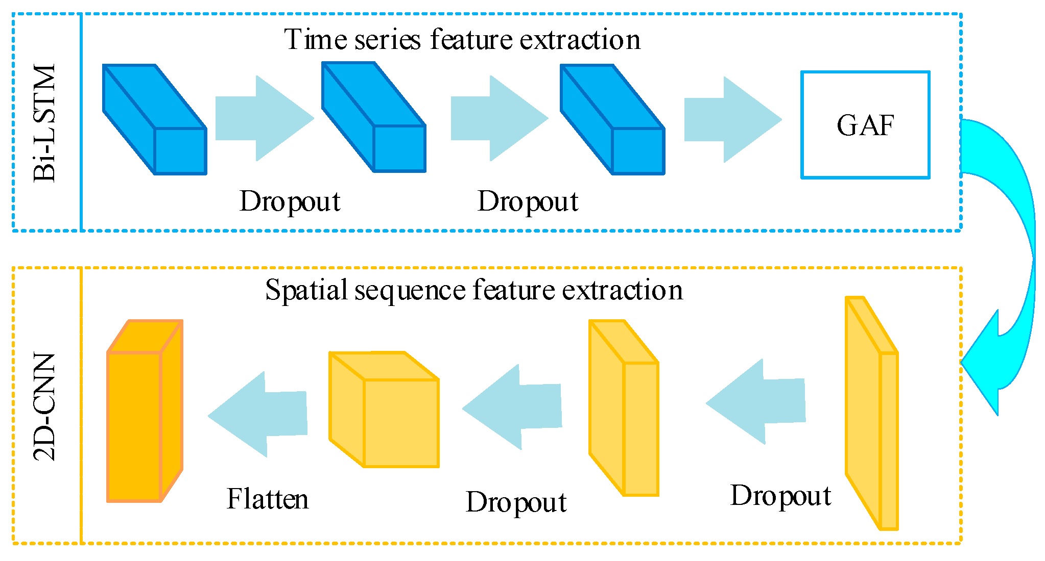
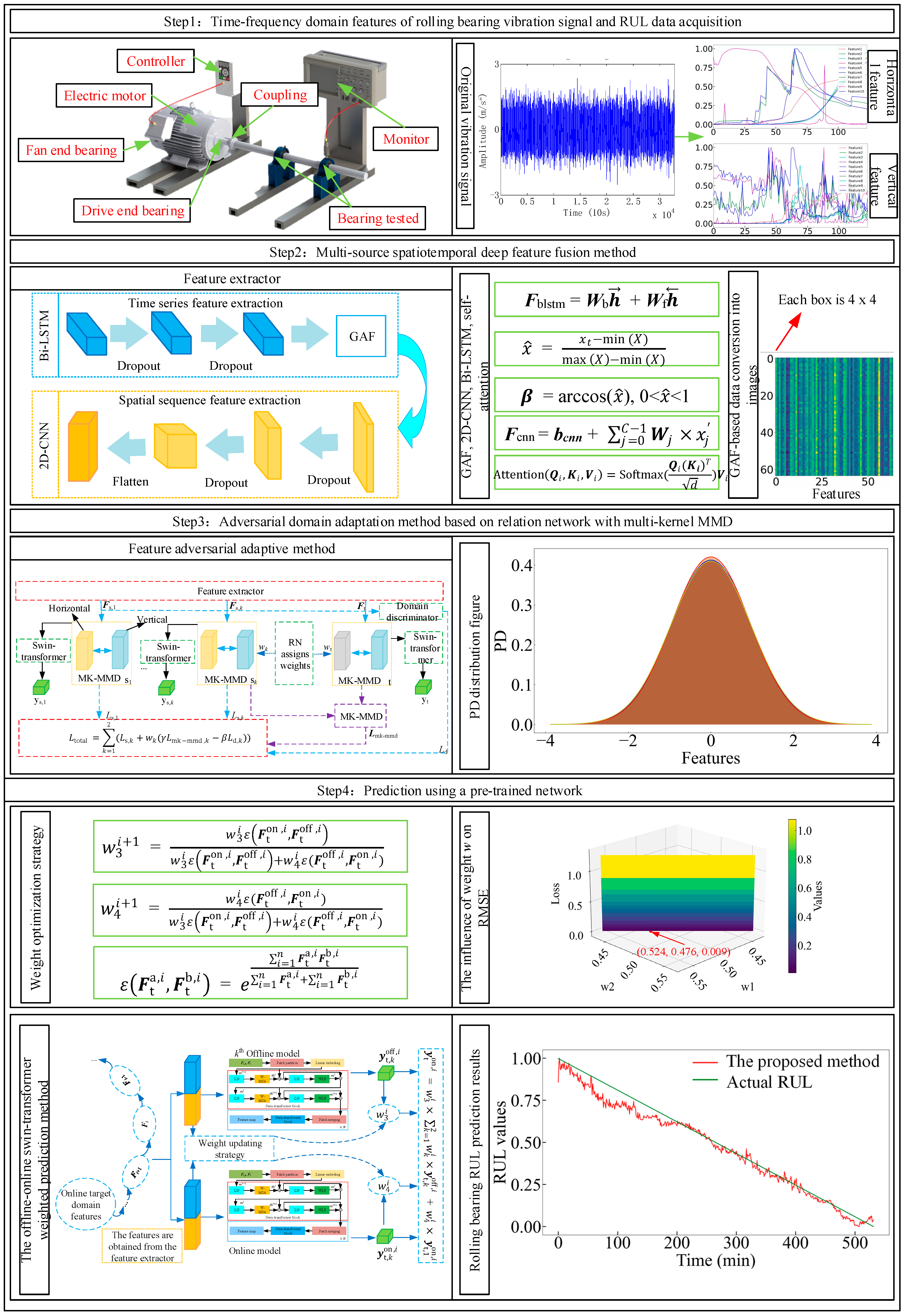
This paper utilizes Bi-LSTM networks to effectively extract emphasize historical features from bearing multi-source time series data. Additionally, a 2D-CNN based on the Gramian Angular Fields (GAF) is employed to capture intricate deep spatial series features. A self-attention mechanism fuses multi-source spatiotemporal feature information to obtain multi-source fusion features. Multi-source spatiotemporal features are extracted jointly for the first time, and a self-attention mechanism is introduced to integrate multi-source spatiotemporal features dynamically to solve the problem of multi-source data redundancy and conflict. The extracted bearing features provide deep multi-source spatiotemporal series features for the model to improve the model’s performance.

(2)

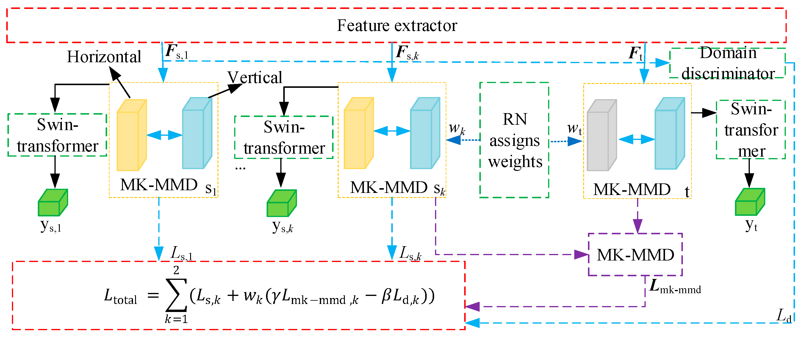
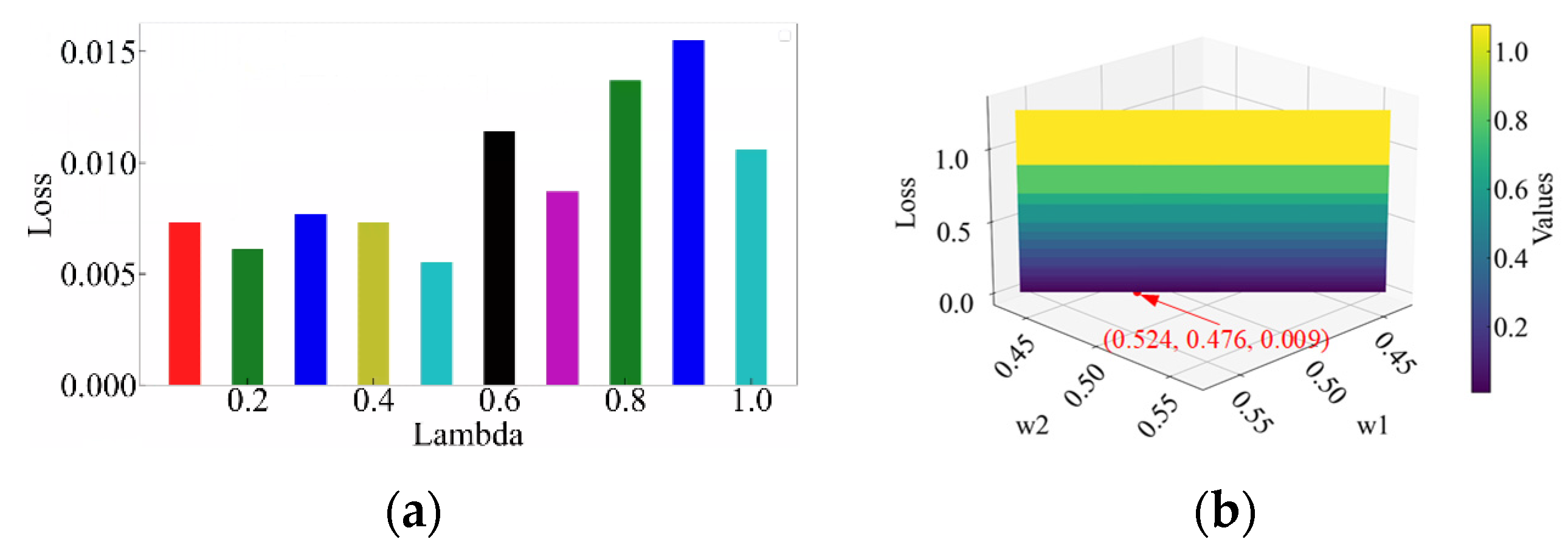
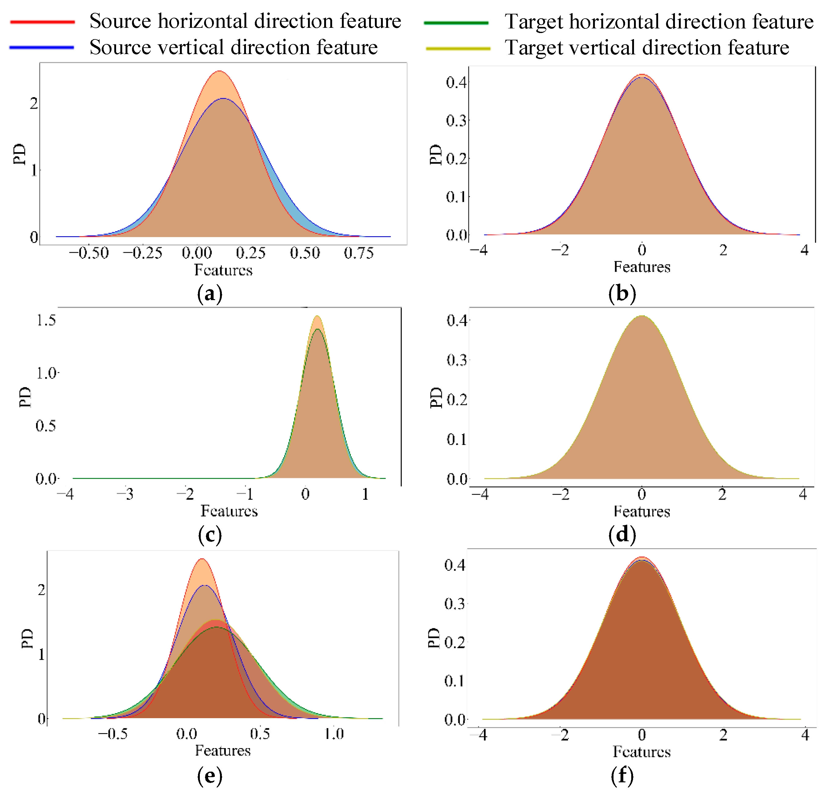
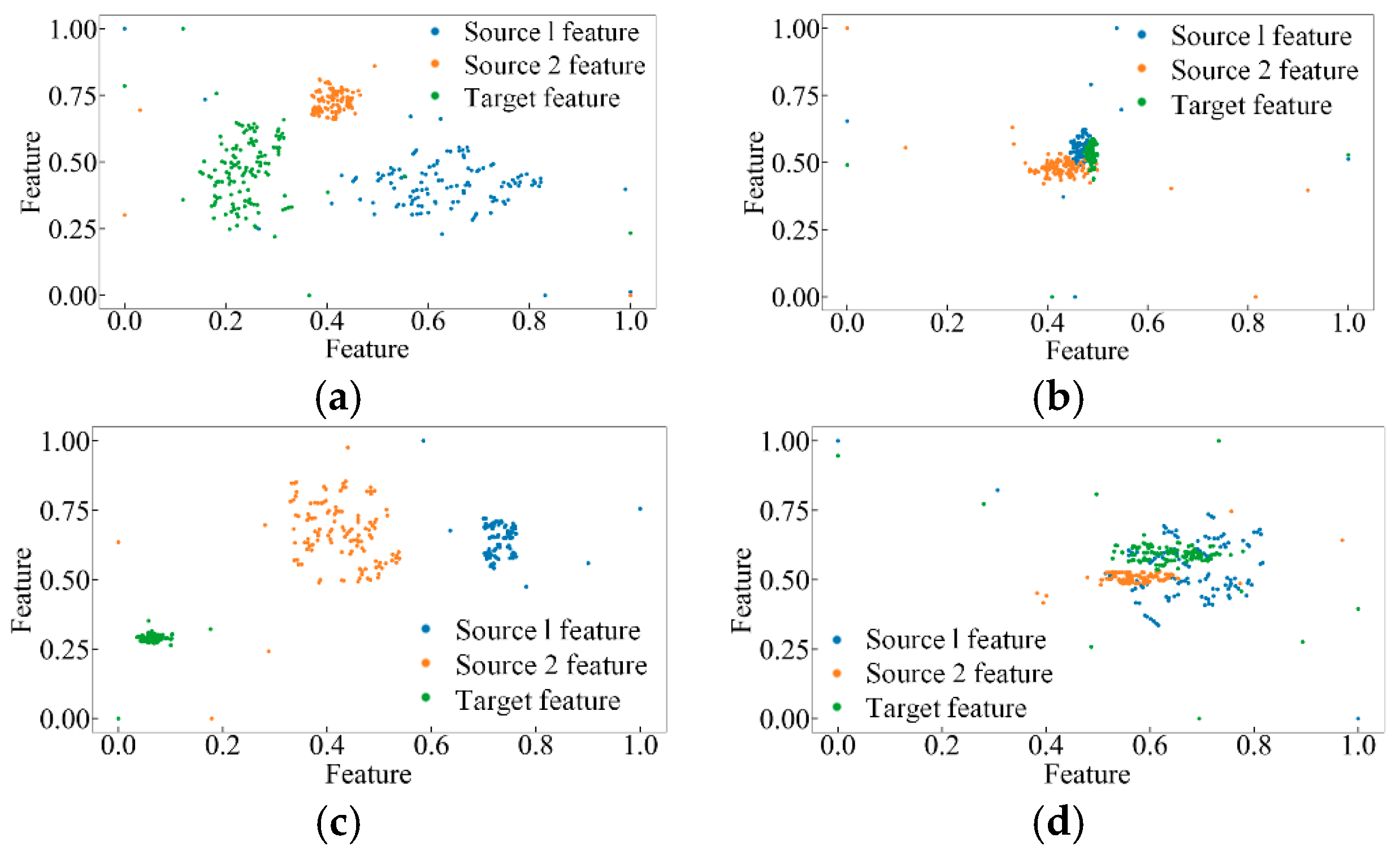
The existing cross-domain methods, such as MMD, only focus on the inter-domain differences and ignore the multi-source feature distribution inconsistency within the domain. A Relational Network Integrated with Maximum Kernel Mean Discrepancy (RN-MK-MMD) is implemented to minimize discrepancies in multi-source feature distributions both inter-domain and intra-domain. This method assigns consistent weights to multi-source features from the multi-source domain and target domain. The adversarial network is introduced to extract cross-domain invariant features to fully learn important bearing degradation features. It is to balance multi-source feature information and improve the model cross-domain bearing important feature extraction.

(3)

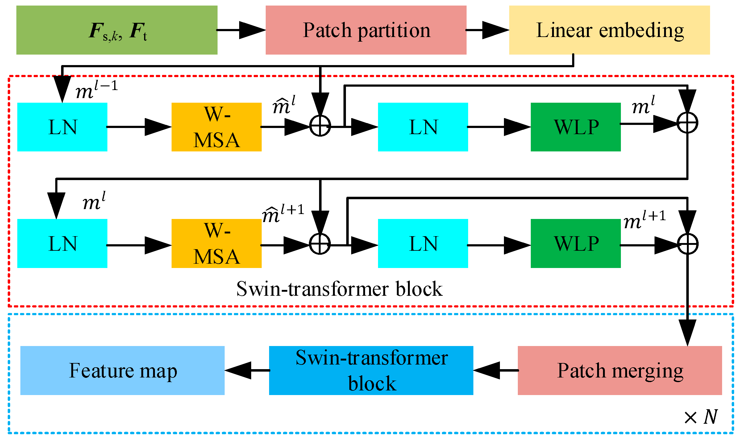
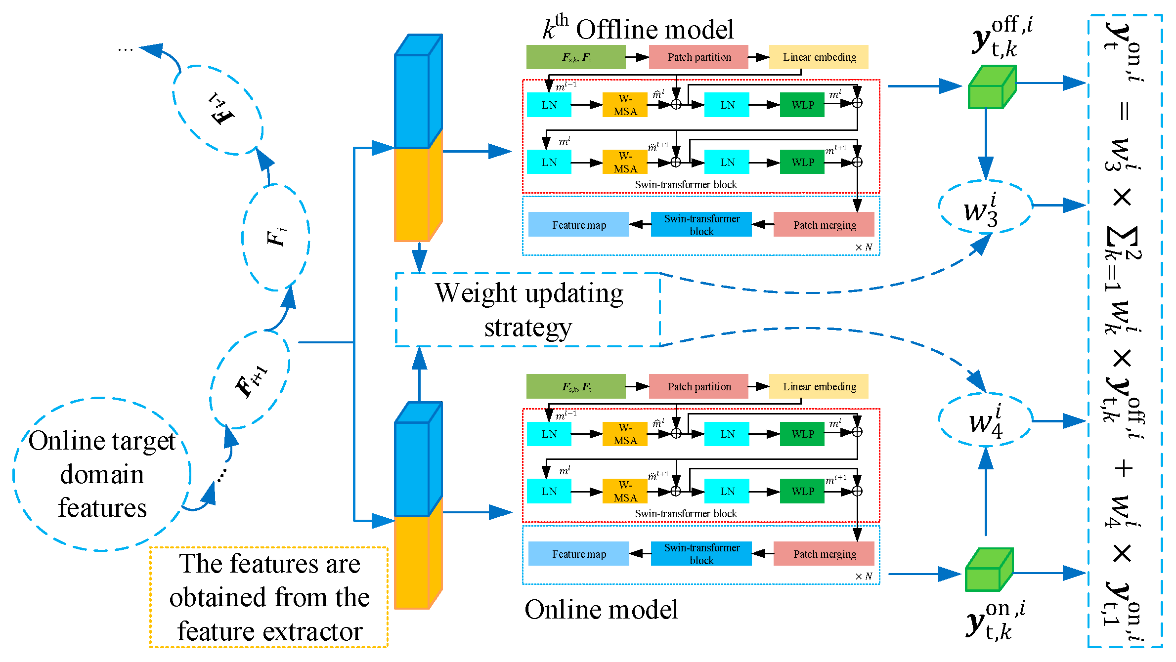
A weight updating strategy is introduced to assign appropriate weights to both offline and online prediction methods based on the swin-transformer. This approach enhances the prediction performance and robustness of the model, ensuring that the model remains adaptable and accurate under varying operational conditions by effectively leveraging real-time and reliable online data.

(4)

The existing work usually deals with multi-source fusion, cross-domain adaptation, or online prediction in isolation, but this framework integrates the three for the first time to realize end-to-end online cross-domain RUL prediction. A novel swin-transformer with multi-source information fusion for an online cross-domain bearing RUL prediction framework is proposed.

The rest of the paper is organized as follows: The multi-source information fusion with adversarial domain adaptive method is detailed in Section 2. Section 3 shows the offline-online swin-transformer prediction method. Section 4 presents the new offline-online bearing RUL prediction method framework. Section 5 shows the experimental results. Section 6 verifies the effectiveness of the proposed method. Finally, conclusions are drawn in Section 7.

2. Multi-Source Information Fusion with Adversarial Domain Adaptive Method

In this paper, the multi-source bearing data format is csv format, which contains horizontal and vertical vibration signal data, and the sampling frequency of different data sets is the same. The rolling bearing original vibration signal contains the multi-source feature data, which is processed by Wavelet Packet Transform (WPT). The original vibration signal from the rolling bearing, containing multi-source feature data, is processed by Wavelet Packet Transform (WPT) [34] to extract stable features, and its time-frequency domain feature X includes Root Mean Square (RMS), impulse factor, clearance factor, kurtosis, crest factor, wave factor, frequency skewness, frequency kurtosis, frequency center, and frequency RMS.

2.1. Multi-Source Spatiotemporal Deep Feature Fusion Method

The multi-source spatiotemporal deep feature fusion method can measure the multi-source spatiotemporal relationship between the multi-source domain and the target domain features. It can improve the spatiotemporal sequence deep feature information fusion by assigning weight to the features. The time-frequency domain feature X of the original vibration signal is normalized. It is input into a Bidirectional Short-Duration Memory Network (Bi-LSTM) [35] and Two-Dimensional Convolutional Neural Network (2D-CNN) [36] to extract the deep features of time series and spatial series. In order to reduce the model parameter calculation, the hidden layers in Bi-LSTM and 2D-CNN add dropout, and the dropout enhances network generalization by randomly deleting hidden neurons. The feature extraction structure is shown in Figure 1.

Compared with LSTM [37], Bi-LSTM has advantages in bidirectional bearing degradation change state feature information transmission and long-time series data processing. Its structure is mainly composed of the input gate, output gate, and forgetting gate. Bi-LSTM can capture the historical and future bearing time-frequency domain feature X deep feature information F_blstm; its calculation formula is shown in (4). In this paper, by setting a 30 s sliding window, the model conducts local bidirectional modeling within each time window. When the window is closed, the incremental model update is performed immediately, which not only retains the context-aware advantages of Bi-LSTM but also meets the timeliness requirements of online learning.

$$\mathit{X}=\left[\begin{array}{c}{x}_{11} x_{12} \cdots x_{1n}\\ x_{21} x_{22} \cdots x_{2n}\\ ⋮\\ x_{m1} x_{m2} \cdots x_{mn}\end{array}\right]$$

(1)

$$\begin{array}{l}{\mathit{C}}_t=\mathsf{\sigma }\left({\mathit{W}}_{\mathrm{fx}}{\mathit{x}}_t+{\mathit{W}}_{\mathrm{fh}}{\mathit{h}}_{t-1}+{\mathit{b}}_{\mathrm{f}}\right)\odot {\mathit{C}}_{t-1}+\mathsf{\sigma }\left({\mathit{W}}_{\mathrm{ix}}{\mathit{x}}_t+{\mathit{W}}_{\mathrm{ih}}{\mathit{h}}_{t-1}+{\mathit{b}}_{\mathrm{i}}\right)\\ +\tan \mathrm{h}\left({\mathit{W}}_{\mathrm{cx}}{\mathit{x}}_t+{\mathit{W}}_{\mathrm{ch}}{\mathit{h}}_{t-1}+{\mathit{b}}_{\mathrm{c}}\right)\end{array}$$

(2)

$$\overrightarrow{\mathit{h}}={\mathit{h}}_t=\mathsf{\sigma }\left({\mathit{W}}_{\mathrm{ox}}{\mathit{x}}_t+{\mathit{W}}_{\mathrm{oh}}{\mathit{h}}_{t-1}+b_{\mathrm{o}}\right)\odot \tan \mathrm{h}\left({\mathit{C}}_{\mathrm{t}}\right)$$

(3)

$${\mathit{F}}_{\mathrm{blstm}}={\mathit{W}}_{\mathrm{b}}\overrightarrow{\mathit{h}}+{\mathit{W}}_{\mathrm{f}}\overleftarrow{\mathit{h}}$$

(4)

where x_t is the vector of the bearing feature matrix X at time step t. X is defined in Equation (1). C_t, h_t represent the Bi-LSTM’s cell state update, cell state, and hidden state at time step t, respectively. As shown in Equations (2)–(4), $\overrightarrow{\mathit{h}}$, $\overleftarrow{\mathit{h}}$ denote the hidden states of the forward and backward Bi-LSTMs, respectively. It has the same calculation process, but the difference is the hidden state h and the cell state C at each layer. $\overleftarrow{\mathit{h}}$ utilizes the previous hidden state h_t−1 and cell state C_t−1. $\overleftarrow{\mathit{h}}$ uses the next hidden state h_t+1 and cell state C_t+1. $\mathsf{\sigma }$ is the sigmoid function. $\odot$ denotes element-wise multiplication. W and b are the model’s weight and bias parameters.

$$\widehat{x}={\displaystyle \frac{x_t-\min \left(\mathit{X}\right)}{\max \left(\mathit{X}\right)-\min \left(\mathit{X}\right)}}$$

(5)

$$\mathit{\beta }=\arccos \left(\widehat{x}\right),0<\widehat{x}<1$$

(6)

$${\mathit{X}}^{\prime }=\left[\begin{array}{c}\cos \left({\beta }_1+{\beta }_1\right)\cos \left({\beta }_1+{\beta }_2\right)\cdots \cos \left({\beta }_1+{\beta }_n\right)\\ \cos \left({\beta }_2+{\beta }_1\right)\cos \left({\beta }_2+{\beta }_2\right)\cdots \cos \left({\beta }_2+{\beta }_n\right)\\ ⋮\\ \cos \left({\beta }_n+{\beta }_1\right)\cos \left({\beta }_n+{\beta }_2\right)\cdots \cos \left({\beta }_n+{\beta }_n\right)\end{array}\right]$$

(7)

In order to extract and enhance the spatial feature information of F_blstm, Gramian Angular Fields (GAF) [38] were used to transform time series features into image features $\mathit{X}\prime$, which can be beneficial to extract $\mathit{X}\prime$ features through 2D-CNN. The 2D-CNN, consisting of a convolution layer and a pooling layer, extracts useful local spatial feature information from ${\mathit{X}}^{\prime }$ to obtain the spatial feature F_cnn; its calculation formula is given in (8).

$$F_{\mathrm{cnn}}=b_{\mathrm{cnn}}+{\displaystyle \sum }_{j=0}^{C-1}{\mathit{W}}_j\times x_j^{\prime }$$

(8)

where $\widehat{x}$ represents the normalized matrix of X, as shown in Equation (5). $\mathit{\beta }$ is the pseudoinverse of $\widehat{x}$, as shown in Equation (6). ${\mathrm{X}}^{\text{′}}=[x_1^{\prime },x_2^{\prime },\cdots ,x_n^{\prime }]$, Equation (7) generates image features through Gramian Angular Summation Field (GASF) matrix; it is used to capture the similarity of time series features. Each $\cos \left({\beta }_1+{\beta }_1\right)$ represents the correlation at different time points, as shown in Equation (7). F_cnn is obtained through a 2D-CNN. W_j and b_j are the weight and bias for the jth feature in the 2D-CNN. C is the total feature dimensions. j is the feature dimension.

The L2 regularization [39] was embedded into the full connection layer of the feature extractor. It can make the parameters of the model small and sparse and captures global feature information, as shown in Equation (9).

$$\underset{\mathit{W}}{\min }(\lambda {\Vert \mathit{W}\Vert }_2+{\displaystyle \frac{1}{2}}\Vert \mathit{Y}-f\left(\mathit{W}{\mathit{F}}^{\prime }-\mathit{b}\right)\Vert )$$

(9)

where $\lambda$ is the regularization parameter.

By extracting the multiple sources horizontal feature ${\mathit{F}}_{\mathrm{s},k}^{\prime }$, vertical feature ${\mathit{F}}_{\mathrm{sv},k}^{\prime }$, target domain horizontal feature ${\mathit{F}}_{\mathrm{th}}^{\prime }$, and vertical feature ${\mathit{F}}_{\mathrm{tv}}^{\prime }$ of the rolling bearing through a feature extractor, it was concatenated to form the feature sequence ${\mathit{F}}_{\mathrm{s},k}^{\prime }$ and ${\mathit{F}}_{\mathrm{t}}^{\prime }$. Then, a self-attention mechanism [40] was employed to assign weights to ${\mathit{F}}^{\prime }$, yielding the fused feature sequence F, as follows:

$${\mathit{F}}_{\mathrm{s},k}^{\prime }=\mathrm{concat}({\mathit{F}}_{\mathrm{sh},k}^{\prime },{\mathit{F}}_{\mathrm{sv},k}^{\prime })$$

(10)

$${\mathit{F}}_{\mathrm{t}}^{\prime }=\mathrm{concat}({\mathit{F}}_{\mathrm{th}}^{\prime },{\mathit{F}}_{\mathrm{tv}}^{\prime })$$

(11)

$${\mathit{Q}}_i={\mathit{F}}_i^{\prime }\times {\mathit{W}}_q$$

(12)

$${\mathit{K}}_i={\mathit{F}}_i^{\prime }\times {\mathit{W}}_{\mathit{k}}$$

(13)

$${\mathit{V}}_i={\mathit{F}}_i^{\prime }\times {\mathit{W}}_v$$

(14)

$$\mathrm{Attention}\left({\mathit{Q}}_i,{\mathit{K}}_i,{\mathit{V}}_i\right)=\mathrm{Softmax}\left({\displaystyle \frac{{\mathit{Q}}_i{\left({\mathit{K}}_{\mathit{i}}\right)}^T}{\sqrt{d}}}\right){\mathit{V}}_i$$

(15)

where Q, K, and V represent the query, key, and value vectors, respectively, while d denotes the dimensionality of the query and key. The attention scores are computed by taking the dot product of Q and K, then dividing by the scaling factor d. These scores are subsequently passed through a softmax function to obtain weights, which are applied to the value vector V to produce the final fused feature sequence F.

2.2. Adversarial Domain Adaptation Method Based on Relation Network with Multi-Kernel MMD

The domain adversarial adaptive method based on Relation Network with Multi-Kernel MMD (RN-MK-MMD) can improve the feature transfer effect. The structural process flow is illustrated in Figure 2. It mainly reduces the difference between the multi-source feature distributions in a multi-source domain, as well as the difference between the feature distribution of the multi-source domain and the target domain, and extracts local and global invariant features.

The Relational Network (RN) combined with the MK-MMD [41] method was used to achieve domain self-adaptation, which can reduce the distribution difference between the kth source domain feature F_s,k, and the target domain feature F_t, and it can extract inter-domain invariant features. The similarity score ${\mathit{\tau }}_k$ between F_s,k and F_t was calculated through RN; it assigns weights w_k to the predicted RUL values, as shown in Equation (18), the prediction loss L_y,k, discriminator loss L_d,k, maximum mean discrepancy L_m,k for the kth source domain. The parameters W_y, W_d, W_f were optimized using cross-entropy to minimize the total loss, as shown in Equation (20). The distance between the source domain features F_s,k and the target domain features F_t was calculated by MK-MMD to reduce the distribution discrepancy across domains. The kth source bearing features $F_{\mathrm{s},k}$ input into the RUL predictor to obtain the prediction y_s,k.

$${\mathit{\tau }}_k=g_{\varnothing }\left(\xi \left({\mathit{F}}_{\mathrm{s},k},{\mathit{F}}_{\mathrm{t}}\right)\right)$$

(16)

$$u_k={\displaystyle \frac{{{\displaystyle \sum }}_{i=0}^{m-1}{\mathit{\tau }}_{k,i}}{m}}$$

(17)

$$w_k={\displaystyle \frac{u_k}{{{\displaystyle \sum }}_{i=1}^2{u}_i}}$$

(18)

$$\begin{array}{l}\mathrm{M}(F_{s,k},F_t)={\displaystyle \frac{1}{N_{\mathrm{s},k}^2}}{\displaystyle \sum _{i=1}^{N_{\mathrm{s},k}}{\displaystyle \sum _{j=1}^{N_{\mathrm{s},k}}k(F_{\mathrm{s},k}^i,F_{\mathrm{s},k}^j)}}+{\displaystyle \frac{1}{N_{\mathrm{t}}^2}}{\displaystyle \sum _{i=1}^{N_{\mathrm{t}}}{\displaystyle \sum _{j=1}^{N_{\mathrm{t}}}k(F_{\mathrm{t}}^i,F_{\mathrm{t}}^j)}}-\\ {\displaystyle \frac{1}{N_{\mathrm{s},k}{N}_{\mathrm{t}}}}{\displaystyle \sum _{i=1}^{N_{\mathrm{s},k}}{\displaystyle \sum _{j=1}^{N_{\mathrm{t}}}k(F_{\mathrm{s},k}^i,F_{\mathrm{t}}^j)}}\end{array}$$

(19)

$$\begin{array}{l}{L}_{\mathrm{total}}(W_{\mathrm{y}},W_{\mathrm{d}},W_{\mathrm{f}})={\displaystyle \sum _{k=1}^2(L_{\mathrm{s},k}(W_{\mathrm{y}},W_{\mathrm{f}})}+w_k(\gamma L_{\mathrm{mk}-\mathrm{mmd},k}(W_{\mathrm{mk}-\mathrm{mmd}},W_{\mathrm{f}})-\\ \beta L_{\mathrm{d},k}(W_{\mathrm{d}},W_{\mathrm{f}})))\end{array}$$

(20)

$$H\triangleq \{K={\displaystyle \sum }_{m=1}^q{a}_m{k}_m:a_m\ge 0,\forall m\}$$

(21)

where $g_{\varnothing }$ represents the correlation calculation. $\xi$ represents the connection function. k is the number of sources, k = 1, 2. w_k represents the RUL prediction weight for the kth source. ${\tau }_k$ and u_k are the similarity score and the average value between the kth source domain and the target domain features, respectively. $\phi (\cdot )$ represents the kernel function. H is the RKHS mapping function. N_s,k and N_t are the number of samples in the kth source domain and target domain, respectively. M ($\cdot$) is the multi-kernel maximum mean discrepancy function, as shown in Equation (19). MK-MMD method can effectively match high- and low-order features by selecting different bandwidth kernels. The different bandwidth core’s contributions are interpreted as appropriate trade-off parameters. The linear combination of different Gaussian kernels is given in Equation (21). W_f represents the feature extraction weight. W_d represents the domain discriminator weight. W_y ($\cdot$) represents the bearing RUL predictor weight. L_mk-mmd,k represents the mk-mmd loss value of the bearing feature in the k-source domain. L_d,k represents the discriminative domain loss value between the kth source domain and the target domain bearing features. $\beta$ and $\gamma$ are parameter balancing coefficients, each set to 0.5. y_s,k is the RUL prediction value. ${\alpha }_i$ is the ith domain maximum mean discrepancy value.

3. The Offline-Online Swin-Transformer Prediction Method

A feature extractor is utilized to obtain the features F_s,k and F_t. An adversarial network, combined with RN-MK-MMD, extracts the shared multi-source features across the target domains. Subsequently, the swin-transformer [28] is employed to learn and capture local information from multi-source common features, enabling the model to focus more on important degradation patterns. The swin-transformer structural is shown in Figure 3. As a result, the proposed approach improves the accuracy of bearing RUL prediction. The self-attention mechanism in the transformer [33] emphasizes global feature information. The transformer has high computational complexity, lacks hierarchical structure, and is weak in capturing local details, which is O(N²). Compared with the transformer, the swin-transformer introduces a sliding-window attention mechanism and a hierarchical structure, which together reduce the model complexity and the complexity to O(M × W²) by local window attention, enable multi-scale feature extraction, and allow the model to better capture local features. The F_s,k and F_t feature map, sized $16\times 1\times 1$, is passed into the first stage of the swin-transformer block after the patch-partition layer. This block contains two subunits: Shifted Window-Based Attention (SW-MSA) and Window-Based Self-Attention (W-MSA). The related calculation formulas are given in [28], primarily aiming to extract local feature information. Subsequently, multiple rounds of feature downsampling are performed in the N-th stage. In addition to the linear embedding layer and the swin-transformer block in the first stage, each subsequent stage comprises a patch-merging layer and another swin-transformer block. In this paper, the features were downsampled four times in the first stage to obtain feature maps with dimensions of $256\times (1/4)\times (1/4)$, and further downsampled eight times in the second stage to achieve $512\times (1/8)\times (1/8)$, Finally, the features $m^{l+1}$ were utilized for predicting the bearings RUL, as shown in Equation (26).

$${\widehat{m}}^l=W-MSA\left(LN\left(m^{\left(l-1\right)}\right)\right)+m^{\left(l-1\right)}$$

(22)

$$m^l=MLP\left(LN\left({\widehat{m}}^l\right)\right)+{\widehat{m}}^l$$

(23)

$${\widehat{m}}^{l+1}=SW-MSA\left(LN\left(m^l\right)\right)+m^l$$

(24)

$$m^{l+1}=MLP\left(LN\left({\widehat{m}}^{l+1}\right)\right)+{\widehat{m}}^{l+1}$$

(25)

$$\mathit{y}=m^{l+1}{\mathit{W}}_{\mathrm{y}}+b_{\mathrm{y}}$$

(26)

where ${\widehat{m}}^l$ and $m^l$ represents the output of SW-MSA and MLP modules, respectively, as shown in Equations (22) and (23). $m^{\left(l-1\right)}$ and $m^{l+1}$ represents the input and output of the swin-transformer block, respectively, as shown in Equations (24) and (25), LN is layer regularization, MLP is multi-layer perceptron, and y is the predicted value of bearing RUL.

The swin-transformer method was trained the way for offline and online, respectively. It can learn offline and online bearing deep features from multi-source spatiotemporal sequence. The structural process flow is illustrated in Figure 4. The offline swin-transformer method is trained using multi-source bearing data, and its structure includes a feature extractor, discriminator, and predictor. The feature extractor parameters of the trained offline method are initialized to those of the online method. The offline and online target bearings RUL predicted values, which were obtained by inputting the target training bearing data streams into the offline and online swin-transformer methods, respectively. The bearing RUL prediction weight $w_3^i$ in the offline method and bearing RUL prediction weight $w_4^i$ in the online method were obtained through Equations (29) and (30). It is used as the next step to obtain the weighted predicted value of the target bearing data flow. The optimal swin-transformer online method is obtained through iterative training. The trained swin-transformer online method is used to obtain the test target bearing RUL prediction value ${\mathit{y}}_{\mathrm{t}}^{\mathrm{on},i}$.

$${\mathit{y}}_t^{\mathrm{on},i}=w_3^i\times \left(w_1^i\times {\mathit{y}}_{\mathrm{t}, 1}^{\mathrm{off},i}+w_2^i\times {\mathit{y}}_{\mathrm{t},2}^{\mathrm{off},i}\right)+w_4^i\times {\mathit{y}}_{\mathrm{t},1}^{\mathrm{on},i}$$

(27)

$$w_3^{i+1}={\displaystyle \frac{w_3^i\epsilon \left({\mathit{F}}_{\mathrm{t}}^{\mathrm{on},i},{\mathit{F}}_{\mathrm{t}}^{\mathrm{off},i}\right)}{w_3^i\epsilon \left({\mathit{F}}_{\mathrm{t}}^{\mathrm{on},i},{\mathit{F}}_{\mathrm{t}}^{\mathrm{off},i}\right)+w_4^i\epsilon \left({\mathit{F}}_{\mathrm{t}}^{\mathrm{off},i},{\mathit{F}}_{\mathrm{t}}^{\mathrm{on},i}\right)}}$$

(28)

$$w_4^{i+1}={\displaystyle \frac{w_4^i\epsilon \left({\mathit{F}}_{\mathrm{t}}^{\mathrm{off},i},{\mathit{F}}_{\mathrm{t}}^{\mathrm{on},i}\right)}{w_3^i\epsilon \left({\mathit{F}}_{\mathrm{t}}^{\mathrm{on},i},{\mathit{F}}_{\mathrm{t}}^{\mathrm{off},i}\right)+w_4^i\epsilon \left({\mathit{F}}_{\mathrm{t}}^{\mathrm{off},i},{\mathit{F}}_{\mathrm{t}}^{\mathrm{on},i}\right)}}$$

(29)

$$\epsilon \left({\mathit{F}}_{\mathrm{t}}^{\mathrm{off},i},{\mathit{F}}_{\mathrm{t}}^{\mathrm{on},i}\right)=e^{{\displaystyle \frac{{{\displaystyle \sum }}_{i=1}^n{\mathit{F}}_{\mathrm{t}}^{\mathrm{off},i}{\mathit{F}}_{\mathrm{t}}^{\mathrm{on},i}}{{{\displaystyle \sum }}_{i=1}^n{\mathit{F}}_{\mathrm{t}}^{\mathrm{off},i}+{{\displaystyle \sum }}_{i=1}^n{\mathit{F}}_{\mathrm{t}}^{\mathrm{on},i}}}}$$

(30)

where $y_{\mathrm{t},k}^{\mathrm{off},i}$ is the ith target domain bearing sample RUL predicted value in the k-source offline model. $y_{\mathrm{t},k}^{\mathrm{on},i}$ is the ith target domain bearing sample RUL predicted value in the k-source online model. It can be seen from Equation (27). $w_1^i$ is the prediction weight of the offline model RUL for the ith bearing sample at source 1. $w_2^i$ is the prediction weight of the online model RUL for the ith bearing sample at source 2. The ith bearing sample RUL predicted weight $w_3^i$ in the offline model was obtained by Equation (28). The ith bearing sample RUL predicted weight $w_4^i$ in the online model was obtained by Equation (29). $\epsilon (\cdot )$ is to calculate the correlation between ${\mathit{F}}_{\mathrm{t}}^{\mathrm{on}}$ and ${\mathit{F}}_{\mathrm{t}}^{\mathrm{off}}$, as seen from Equation (30).

4. The Proposed Method

An online cross-domain bearings RUL prediction method based on a swin-transformer with multi-source information fusion is illustrated in this work. This method effectively extracts and fuses the multi-source spatiotemporal sequence deep features of the rolling bearing and improves the RUL prediction performance. The implementation steps are as follows:

Step 1: The original bearing vibration signal is processed by WPT noise reduction. Its time-frequency domain features are used as original features and input to the feature extractor for feature extraction.

Step 2: The Bi-LSTM extracts the bearing time series features. The GAF converts the time series feature into image data sets, which are input into 2D-CNN to extract the spatial series deep features. The self-attention mechanism fuses multi-source spatiotemporal feature information to obtain multi-source fusion features.

Step 3: The RN-MK-MMD method reduces the distribution difference between multi-source domain and target domain features, embedding the cross-domain adversarial method to extract invariant features.

Step 4: The swin-transformer trains the fused multi-source features, fully combining historical empirical data and real-time data to construct the offline-online bearing RUL prediction model. The weight update strategy optimizes the prediction weight of the offline-online model.

Figure 5 illustrates the specific framework.

5. Experimental Verification

5.1. Case1: XJTU-SY Dataset

The XJTU-SY dataset [42] was used to verify the feasibility of the proposed method, which comes from Xi’an Jiaotong University (Xi’an, China) and Changxing Shengyang Technology (Huzhou, China). The sampling frequency was set to 25.6 kHz, with a sampling interval of 1 min and a duration of 1.28 s per sample. The dataset contains 15 run-to-failure bearings under three different operating conditions. A portion of the bearing fault data is shown in

Table 1. Case 1 experimental settings.

Task	Transfer Scenario	Offline Dataset in Source Domain	Number of Data	Online Dataset in Target Domain	Number of Data	Testing Dataset in Target Domain	Number of Data
XT1	I, II $\to$ III	S1:XB11, S2:XB21	123, 491	XB31	2538	XB33	371
XT2	I, III $\to$ II	S1:XB11, S2:XB31	123, 2538	XB21	491	XB23	533
XT3	II, III $\to$ I	S1:XB21, S2:XB31	161, 2496	XB11	123	XB13	158

. The rolling bearing dataset is divided into a training set and a test set, with the verification set comprising 20% of the training set. By analyzing the results of the training loss curve in Figure 6, the domain loss decreases most rapidly before the epoch is 20. This is followed by the balance coefficient Lambda domain loss, total loss, and regression loss. After epoch 20, the Lambda domain loss associated with the balance coefficient decreases the fastest. It is followed by domain loss, total loss, and regression loss, and finally, each loss curve stabilizes.

Task XT1 was used to verify the influence of multi-source domain features similarity weight distribution and Lamada coefficient on the training loss of the predictive model. As shown in Figure 7, the different Lambdas have different loss bar heights. The training losses are minimized when Lambda is 0.5, as presented in Figure 7a. The multi-source domain similarity weights w1 and w2 are represented by different colors, with each color corresponding to a different loss value. When w1 and w2 are 0.524 and 0.476, respectively, the minimum loss value is 0.009, as presented in Figure 7b.

Figure 8 shows the effect of the RN-MK-MMD method on balancing the multi-source domain and the target domain horizontal and vertical direction features PD distribution in task XT3. The PD distribution difference between horizontal and vertical features remains obvious, even before applying the RN-MK-MMD method. As shown in Figure 8a,c, the PD distributions of horizontal and vertical features basically overlap in Figure 8b,d, even after adopting the RN-MK-MMD method. It demonstrates the feasibility of the RN-MK-MMD method. Comparative analysis of Figure 8e shows that the RN-MK-MMD method can make the multi-source domain and target domain horizontal and vertical feature PD distributions similar, but the multi-source domain and target domain feature PD distribution is different. Thus, the RN-MK-MMD method reduces the difference in the inter-domain feature distribution. The PD distribution of features from the multi-source domain and target domain is clearly similar in Figure 8f. This provides a basis for the prediction model to extract domain-invariant features and improve performance.

Figure 9 evaluates the impact of the RN-MK-MMD method on the feature distribution across multi-source domain and target domain in tasks XT1 and XT2. In Figure 9a,c, the features were scattered and dissimilar before the RN-MK-MMD method was applied. This makes domain-invariant feature extraction difficult. In Figure 9b,d, the features were clustered and similar after applying the RN-MK-MMD method. This reduces the difference in inter-domain feature distribution, enabling the prediction model to better extract domain invariant features.

To verify the feasibility of the online prediction model based on the swin-transformer, Figure 10 shows the impact of the different offline and online prediction model prediction weights on the training loss of the swin-transformer online prediction model. The training loss reaches its lowest value of 0.002 when the w3 and w4 are 0.527 and 0.473, respectively. This shows that the training loss value changes with the variations in w3 and w4 and that these weights significantly impact the model’s training loss.

Figure 11 shows that the predicted curve of the proposed method is close to the actual curve of the test sample set in tasks XT1 and XT2. The predicted curve at task XT2 performs better than that at task XT1, and the results prove the feasibility of the proposed method.

5.2. Case2: PHM2012 Dataset

The PHM2012 dataset [43] was used to verify the feasibility of the proposed method. The sampling frequency was set at 25.6 kHz, the sampling interval was 10 s, and each sampling duration was 0.1 s. Data were collected on the PRONOSTIA platform and include 17 run-to-failure bearings under three different operating conditions. Part of the bearing fault data partitioning is shown in

Table 2. Case 2 experimental settings.

Task	Transfer Scenario	Offline Dataset in Source Domain	Number of Data	Online Dataset in Target Domain	Number of Data	Testing Dataset in Target Domain	Number of Data
PT1	I, II $\to$ III	S1:PB11, S2:PB21	2803, 911	PB31	515	PB32	1637
PT2	I, III $\to$ II	S1:PB11, S2:PB31	2803, 515	PB21	911	PB22	797
PT3	II, III $\to$ I	S1:PB21, S2:PB31	911, 515	PB11	2803	PB12	871

. The rolling bearing data set is divided into training sample set and test sample set, in which the verification sample set accounts for 20% of the training sample set. Analysis of the proposed method training loss curve is shown in Figure 12. The domain loss decreased most rapidly, followed by the Lambda domain loss, total loss, and regression loss, and each loss curve tends to be stable.

Task PT1 was used to verify the influence of multi-source feature similarity weight and Lambda on the predictive model training loss. According to the analysis of the results in Figure 13, the training loss reaches the minimum when the Lambda is 0.5, as shown in Figure 13a. In the 3D plot of Figure 13b, the predicted loss value changes with the variation of multi-source feature similarity weights w1 and w2. When w1 and w2 are 0.494 and 0.506, respectively, the minimum loss value is 0.002.

Figure 14 demonstrates the effect of the RN-MK-MMD method on balancing the multi-source domain and the target domain horizontal and vertical direction features PD distribution in task PT3. Prior to applying the RN-MK-MMD method, the PD distribution of horizontal and vertical features show minimal overlap, as seen in Figure 14a,c. However, after applying the RN-MK-MMD method, the PD distributions of horizontal and vertical features have a high degree of overlap, as shown in Figure 14b,d, indicating the effectiveness of the method. According to the comparative analysis of Figure 14e, it is evident that the RN-MK-MMD method can make the multi-source domain and target domain horizontal and vertical feature PD distributions similar, but the multi-source domain and target domain feature PD distribution is different. Therefore, the RN-MK-MMD method is used to reduce the difference in the inter-domain feature distribution. The multi-source domain and target domain feature PD distribution, which is obviously similar in Figure 14f. It can provide a basis for the prediction model to extract domain invariant features and improve the prediction performance.

Figure 15 evaluates the impact of the RN-MK-MMD method on the feature distribution across multi-source domains and target domains in tasks PT1 and PT2. The features were scattered in Figure 15a,c when the RN-MK-MMD method was applied before, which hindered the model’s ability to extract domain-invariant features. In contrast, the features were clustered, and the shape is elliptical in Figure 15b,d. It can reduce the difference in inter-domain feature distribution. The very close distance between feature clusters further proves that the feature extraction method can extract domain invariant features well.

To verify the feasibility of the online prediction model based on the swin-transformer. Figure 16 illustrates the impact of the different offline and online prediction model prediction weights on the training loss of the swin-transformer online prediction model. The training loss reaches the lowest value of 0.0004 when the w3 and w4 are 0.477 and 0.523, respectively. It shows that the training loss varies with changes in the prediction weights w3 and w4, and the prediction weight value has a significant impact on the online prediction model training loss.

As shown in Figure 17, the predicted curve generated by the proposed method closely matches the actual curve of the test sample set in tasks PT1 and PT2. The predicted curve at task PT1 is better than that at task PT2, demonstrating the feasibility of the proposed method.

6. Comparative Analysis

6.1. Model Parameter Description and Experimental Setup

Experiments validating the feasibility and generalization of the proposed method further demonstrate its effectiveness.

Table 3. Framework structure of the proposed method.

Module	Layer(s)	Kernl /Hidden Size	Stride	Padding	Activation	Input	Output
Feature extractor	Bi-LSTM	128	/	/	ReLu	N × 10	N × 128
	GAF	/	/	/	/	N × 128	N × 8 × 4 × 4
	Convolution	3	1	1	ReLu	N × 8 × 4 × 4	N × 16 × 4 × 4
	Max Pooling	3	2	0	/	N × 16 × 4 × 4	N × 16 × 1 × 1
	Concatenate	horizontal and vertical features			/	N × 16 × 1 × 1, N × 16 × 1 × 1	N × 32 × 1 × 1
	Self-attention	/	/	/	/	N × 32 × 1 × 1	N × 32 × 1 × 1
RUL regression	Swin-transformer	/	/	/	/	N × 32 × 1 × 1	N × 512 × (1/4) × (1/4)
		/	/	/	/	N × 512 × (1/4) × (1/4)	N × 1024 × (1/8) × (1/8)
		128	/	/	/	N × 1024 × (1/8) × (1/8)	N × 128
	Concatenate	Total feature			/	N × 128, N × 128	N × 256
	Dense	32	/	/	ReLU	N × 256	N × 32
	Dense	1	/	/	ReLU	N × 256	N × 1
Domain classification	Dense	32	/	/	ReLU	N × 256	N × 32
	Output	2	/	/	Softmax	N × 32	N × 2

lists the proposed method for each layer network structure parameter values, including the input layer, Bi-LSTM layer, convolutional layer, maximum pooling layer, concatenation layer, full connection layer, swin-transformer, and classification output layer. The network parameters of the proposed method include learning rate, batch size, maximum training epochs, weight optimization function, transfer balance coefficient, and sliding window length, as shown in

Table 4. Hyperparameter settings of the proposed method.

Hyperparameters	Values
Learning rate	0.001
Batch size	64
Max epoch	100
Weight optimization	mini-batch SGD
Transfer coefficient	0.5
window_size	5

. The description of the publicized methods and introduction are shown in

Table 5. Description of comparison methods.

Comparison Method	Description
Baseline [28]	The prediction model without TL; verifies the transferring performance of other TL-based methods.
Deep subdomain adaptation time-quantile regression network (DSATQRN) [31]	These methods are the domain adaptation methods; it can be used to evaluate the performance of the proposed method.
Dual-branch transformer with gated cross attention (DTGCA) [32]	These methods are the different domains’ integrated features methods; it can be used to evaluate the effectiveness of bearing multi-source feature information fusion method.
TCN-transformer [33]	These methods have good predictive performance; it can be used to evaluate the computational complexity, reliability, and effectiveness of the model.
Scheme 1	The Bi-LSTM module is removed.
Scheme 2	The GAF-2D-CNN module is removed.
Scheme 3	The RN-MK-MMD module is removed.
Scheme 4	Replace dynamic update weights with fixed weights.
Scheme 5	Replace swin-transformer with transformer.

. It includes the Baseline [28], DSATQRN [31], DTGCA [32], TCN-transformer [33], and five schemes. The performance of the proposed method and the publicized method was evaluated by using Root Mean Square Error (RMSE), and Mean Absolute Error (MAE). It can be seen from Equations (31) and (32).

$$RMSE=\sqrt{{\displaystyle \frac{1}{n}}{\displaystyle \sum }_{i=1}^n{\left(y_i-\widetilde{y_i}\right)}^2}$$

(31)

$$MAE={\displaystyle \frac{1}{n}}{\displaystyle \sum }_{i=1}^n\left|{\displaystyle \frac{y_i-\widetilde{y_i}}{y_i}}\right|$$

(32)

where $\widetilde{y_i}$ and $y_i$ denote the predicted and actual values of bearing RUL, respectively. n denotes the number of bearing data. The smaller the RMSE and MAE, the better the prediction performance of the prediction model.

6.2. Comparison of Different Adaptive Methods

Task XT3 was used to compare the distribution effect of the multi-source domain and target domain feature points between the proposed method and the publicized methods. Analysis of the t-SNE results shown in Figure 18 reveals the following: In the MMD method, the feature clusters are clustered, but the shapes of the multi-source and target domain feature clusters are not similar. In the MK-MMD method, the target domain feature cluster is clustered close to the source 1 feature cluster, but it remains distant from the source 2 feature cluster, and its shape is not similar. In the MMD-CORAL method, the distribution shape of the multi-source domain and target domain feature clusters is different, and the distance between the clusters is far. Comparing the proposed method with the publicized methods, the feature points of the multi-source domain and target domain are more clustered, and the distance between feature clusters is closer. It verifies the effectiveness of the proposed RN-MK-MMD method.

The distribution effect of multi-source and target bearing feature points of the test sample set in task PT3 is compared between the proposed method and the publicized method. Analysis of the t-SNE results in Figure 19 shows the following: In the MMD method, the feature clusters are clustered, but the shape is not similar. In the MK-MMD method, each cluster feature shape is similar and the source 2 cluster is clustered with the target domain feature cluster, but the distance between the source 1 cluster and the source 2 cluster is far away. In the DTGCA method, the distribution shape of the multi-source domain and target domain feature clusters is roughly similar, but the distance between the source 1 and source 2 clusters is large. In contrast, the feature points of the multi-source domain and target domain in the proposed method are more clustered than the publicized methods. It verifies the effectiveness of the proposed RN-MK-MMD method.

6.3. Comparison of Prediction Methods

The results from the test sample sets in tasks XT3 and PT3 are shown in Figure 20. The prediction curve of the proposed method fits the actual curve better than the publicized prediction methods. As seen in Figure 20a, the TCN-Transformer method provides a better fit than the Baseline, DSATQRN, and DTGCA methods. From Figure 20b, when the time scale is before 200, the Baseline prediction method has a better fitting performance to the actual curve than the TCN-transformer, DSATQRN, and DTGCA prediction methods. After the time scale is 200, the TCN-transformer method has a better fitting performance than Baseline, DTGCA, and DSATQRN prediction methods. Despite this, the proposed method has a better fitting effect than the publicized methods, which verifies the effectiveness of the proposed method. At the end of the bearing RUL in the PT3 task, the RUL value curve suddenly increased significantly, which was due to the data collected from PT3 during rapid bearing degradation failures, the equipment exhibits significant nonlinearity in the late stages of operation. This results in a large disparity between the source and target domains, ultimately impacting the prediction accuracy of PT3.

The computational complexity and runtime of the proposed model compared to the existing models in task XT3 are presented in

Table 6. Efficiency analysis of different methods.

Metrics	Proposed Methos	TCN-Transformer	Baseline	DSATQRN	DTGCA
FLOPs	685.3K	9652.4 K	2894.7 K	2055.6 K	1725.9 K
Params	42.4 K	182.5 K	106.1 K	82.68 K	65.3 K
GPU	1.76 s	3.56 s	1.92 s	1.87 s	1.98 s
CPU	6.89 s	40.58 s	15.68 s	15.23 s	10.02 s

Note: FLOPs represents floating-point arithmetic; it measures the computational complexity of the model. Params reflect the spatial complexity of the model. The GPU and CPU reflect the actual running time of the model in hardware and software, respectively.

. Compared with the TCN-transformer, the proposed model is lower in terms of FLOPs, Params, GPU, and CPU, which are 92.9%, 76.8%, 44.4%, and 83%, respectively. It implements significantly less FLOP, Params, and runtime. DTGCA outperforms the transformer and DSATQRN in terms of FLOPs, Params, GPU, and CPU. Compared to DTGCA, the proposed method reduces FLOPs by 60.3% FLOPs, 35.1% Params, 11.1% GPU, and 31.2% CPU. The experimental results show that the proposed method can significantly reduce both computational costs and storage requirements.

The predictive performance of the proposed method across tasks XT1, XT2, and XT3 is shown in

Table 7. Comparison results of the target domain testing dataset in the XJTU-SY dataset.

Metrics	Model	XT1	XT2	XT3	Average
MAE	Proposed methods	0.044	0.036	0.040	0.040
	Baseline	0.098	0.077	0.099	0.091
	DSATQRN	0.104	0.046	0.074	0.075
	DTGCA	0.079	0.071	0.092	0.081
	TCN-transformer	0.069	0.062	0.073	0.068
	Scheme 1	0.052	0.045	0.048	0.048
	Scheme 2	0.050	0.042	0.046	0.046
	Scheme 3	0.048	0.040	0.044	0.044
	Scheme 4	0.047	0.039	0.043	0.043
	Scheme 5	0.049	0.041	0.045	0.045
RMSE	Proposed methods	0.063	0.049	0.054	0.055
	Baseline	0.112	0.086	0.120	0.106
	DSATQRN	0.121	0.054	0.087	0.087
	DTGCA	0.095	0.079	0.114	0.096
	TCN-transformer	0.086	0.080	0.092	0.086
	Scheme 1	0.075	0.060	0.065	0.067
	Scheme 2	0.070	0.055	0.060	0.062
	Scheme 3	0.068	0.053	0.058	0.060
	Scheme 4	0.066	0.052	0.052	0.058
	Scheme 5	0.069	0.054	0.059	0.061

. The TCN-transformer prediction method outperforms the Baseline, DTGCA, and DSATQRN prediction methods in terms of the average values of MAE, and RMSE. However, compared with the TCN-transformer prediction method, the proposed method in this paper improves the average MAE, and RMSE by 41.2%, and 36%, respectively. It enhances the model’s ability to capture fine-grained spatial-temporal features through its hierarchical attention mechanism compared to the TCN-transformer, which relies solely on temporal convolutions. Among the proposed schemes, Scheme 1 and Scheme 2 show the greatest variation in RMSE and MAE metrics, which indicates that these two schemes have the greatest impact on the model performance, indicating that the dual extraction of spatio-temporal features is the core innovation of the model. Scheme 3 has a smaller effect on performance but still plays an important role, indicating that cross-domain alignment contributes significantly to the generalization ability of the model. The substitution of options 4 and 5 had a slight but significant effect on performance, confirming their role in improving model robustness and computational efficiency. It verifies the advantages of the proposed method in better prediction performance.

The predictive performance of the proposed method across tasks PT1, PT2, and PT3 is shown in

Table 8. Comparison results of the target domain testing dataset in the PHM2012 dataset.

Metrics	Model	PT1	PT2	PT3	Average
MAE	Proposed methods	0.023	0.042	0.051	0.039
	Baseline	0.098	0.133	0.138	0.123
	DSATQRN	0.035	0.085	0.133	0.084
	DTGCA	0.066	0.068	0.128	0.087
	TCN-transformer	0.045	0.072	0.118	0.078
	Scheme 1	0.028	0.050	0.060	0.046
	Scheme 2	0.026	0.048	0.057	0.044
	Scheme 3	0.025	0.046	0.055	0.042
	Scheme 4	0.024	0.045	0.054	0.041
	Scheme 5	0.027	0.049	0.058	0.045
RMSE	Proposed methods	0.031	0.059	0.066	0.052
	Baseline	0.116	0.144	0.172	0.144
	DSATQRN	0.046	0.102	0.154	0.101
	DTGCA	0.071	0.082	0.147	0.100
	TCN-transformer	0.062	0.080	0.140	0.094
	Scheme 1	0.037	0.068	0.075	0.060
	Scheme 2	0.035	0.065	0.072	0.057
	Scheme 3	0.034	0.063	0.070	0.056
	Scheme 4	0.033	0.062	0.069	0.055
	Scheme 5	0.036	0.066	0.073	0.058

. The TCN-transformer prediction method outperforms the Baseline, DTGCA, and DSATQRN prediction methods in terms of the average values of MAE, and RMSE. However, compared with the TCN-transformer prediction method, the proposed method in this paper improves the average MAE, and RMSE by 50%, and 44.7%, respectively. Among the proposed schemes, Scheme 1 and Scheme 2 have the greatest impact on model performance, followed by Scheme 4 and Scheme 5, and Scheme 3 has a slightly smaller impact, but it still contributes significantly. These results validate the advantages of the proposed method in better prediction performance.

7. Conclusions

In this study, a swin-transformer with multi-source information fusion for the online cross-domain bearings RUL prediction method was proposed. The model aims to extract multi-source spatiotemporal features from both source and target domains while minimizing the distribution differences between intra-domain and inter-domain features. The multi-source spatiotemporal deep feature extraction fusion method can extract the intrinsic feature information of the bearing spatiotemporal sequence and the relationship between the feature points, ultimately yielding a fused a multi-source feature. The domain adversarial adaptive method based on the RN-MK-MMD can reduce the distribution difference between the intra-domain and inter-domain multi-source features. The multi-source feature similarity weights w1 and w2 are 0.524 and 0.476, respectively, and the balance coefficient Lambda is 0.5. The RMSE of the offline prediction model based on swin-transformer is about 0.006, which can improve the model prediction performance. The offline and online prediction methods based on the swin-transformer obtained the offline model prediction weight w3 and online model prediction weight w4 of the target domain bearing data flow through the weight updating strategy, which was 0.527 and 0.473, respectively. Its prediction curve fits the actual curve. The proposed prediction method on the XJTU-SY dataset and PHM2012 dataset in terms of MAE were 0.040 and 0.039, and RMSE were 0.055 and 0.052 respectively. These results verify the feasibility, generalization, and effectiveness of the proposed method.

Although the methodology explored here offers valuable insights, it still faces certain constraints, notably its dependence on high-quality multi-source data. Further studies could seek to enhance the deep feature fusion methods for cross-domain multi-source data integration, especially in scenarios of offline data and online data imbalance and weight update strategy optimization, while still maintaining high-precision feature alignment and prediction.

References

1. Wang, H.; Chen, J.; Qu, J.; Ni, G. A new approach for safety life prediction of industrial rolling bearing based on state recognition and similarity analysis. Saf. Sci. 2020, 122, 104530. [Google Scholar] [CrossRef]
2. Siahpour, S.; Li, X.; Lee, J. A novel transfer learning approach in remaining useful life prediction for incomplete dataset. IEEE Trans. Instrum. Meas. 2022, 71, 3509411. [Google Scholar] [CrossRef]
3. Zou, Y.; Li, Z.; Liu, Y.; Zhao, S.; Liu, Y.; Ding, G. A method for predicting the remaining useful life of rolling bearings under different working conditions based on multi-domain adversarial networks. Measurement 2022, 188, 110393. [Google Scholar] [CrossRef]
4. Pan, T.; Chen, J.; Ye, Z.; Li, A. A multi-head attention network with adaptive meta-transfer learning for RUL prediction of rocket engines. Reliab. Eng. Syst. Saf. 2022, 225, 108610. [Google Scholar] [CrossRef]
5. Ren, L.; Sun, Y.; Cui, J.; Zhang, L. Bearing remaining useful life prediction based on deep autoencoder and deep neural networks. J. Manuf. Syst. 2018, 48, 71–77. [Google Scholar] [CrossRef]
6. Huang, C.G.; Zhu, J.; Han, Y.; Peng, W. A novel bayesian deep dual network with unsupervised domain adaptation for transfer fault prognosis across different machines. IEEE Sens. J. 2022, 22, 7855–7867. [Google Scholar] [CrossRef]
7. Li, Z.; Zhang, K.; Liu, Y.; Zou, Y.; Ding, G. A novel remaining useful life transfer prediction method of rolling bearings based on working conditions common benchmark. IEEE Trans. Instrum. Meas. 2022, 71, 3524909. [Google Scholar] [CrossRef]
8. Miao, M.; Yu, J.; Zhao, Z. A sparse domain adaption network for remaining useful life prediction of rolling bearings under different working conditions. Reliab. Eng. Syst. Saf. 2022, 219, 108259. [Google Scholar] [CrossRef]
9. Zhuang, J.; Jia, M.; Zhao, X. An adversarial transfer network with supervised metric for remaining useful life prediction of rolling bearing under multiple working conditions. Reliab. Eng. Syst. Saf. 2022, 225, 108599. [Google Scholar] [CrossRef]
10. Berghout, T.; Mouss, L.H.; Bentrcia, T.; Benbouzid, M. A semi-supervised deep transfer learning approach for rolling-element bearing remaining useful life prediction. IEEE Trans. Energy Conver. 2022, 37, 1200–1210. [Google Scholar] [CrossRef]
11. Mao, W.; Liu, J.; Chen, J.; Liang, X. An interpretable deep transfer learning-based remaining useful life prediction approach for bearings with selective degradation knowledge fusion. IEEE Trans. Instrum. Meas. 2022, 71, 3508616. [Google Scholar] [CrossRef]
12. Hu, T.; Guo, Y.; Gu, L.; Zhou, Y.; Zhang, Z.; Zhou, Z. Remaining useful life estimation of bearings under different working conditions via Wasserstein distance-based weighted domain adaptation. Reliab. Eng. Syst. Saf. 2022, 224, 108526. [Google Scholar] [CrossRef]
13. Hu, T.; Guo, Y.; Gu, L.; Zhou, Y.; Zhang, Z.; Zhou, Z. Remaining useful life prediction of bearings under different working conditions using a deep feature disentanglement based transfer learning method. Reliab. Eng. Syst. Saf. 2022, 219, 108265. [Google Scholar] [CrossRef]
14. Ye, Z.; Yu, J. A selective adversarial adaptation network for remaining useful life prediction of machines under different working conditions. IEEE Syst. J. 2023, 17, 62–71. [Google Scholar] [CrossRef]
15. Rathore, M.S.; Harsha, S.P. Rolling bearing prognostic analysis for domain adaptation under different operating conditions. Eng. Fail. Anal. 2022, 139, 106414. [Google Scholar] [CrossRef]
16. Ding, Y.; Ding, P.; Zhao, X.; Cao, Y.; Jia, M. Transfer learning for remaining useful life prediction across operating conditions based on multisource domain adaptation. IEEE-ASME Trans. Mechatron. 2022, 27, 4143–4152. [Google Scholar] [CrossRef]
17. Zhu, R.; Peng, W.; Wang, D.; Huang, C.G. Bayesian transfer learning with active querying for intelligent cross-machine fault prognosis under limited data. Mech. Syst. Signal Process. 2023, 183, 109628. [Google Scholar] [CrossRef]
18. Huang, C.G.; Huang, H.Z.; Li, Y.F.; Peng, W. A novel deep convolutional neural network-bootstrap integrated method for RUL prediction of rolling bearing. J. Manuf. Syst. 2021, 61, 757–772. [Google Scholar] [CrossRef]
19. Mao, W.; Liu, K.; Zhang, Y.; Liang, X.; Wang, Z. Self-supervised deep tensor domain-adversarial regression adaptation for online remaining useful life prediction across machines. IEEE Trans. Instrum. Meas. 2023, 72, 2509916. [Google Scholar] [CrossRef]
20. Yang, J.; Wang, X. Meta-learning with deep flow kernel network for few shot cross-domain remaining useful life prediction. Reliab. Eng. Syst. Saf. 2024, 244, 109928. [Google Scholar] [CrossRef]
21. Xiang, S.; Li, P.; Luo, J.; Qin, Y. Micro transfer learning mechanism for cross-domain equipment rul prediction. IEEE Trans. Autom. Sci. Eng. 2024, 22, 1460–1470. [Google Scholar] [CrossRef]
22. Dong, S.; Xiao, J.; Hu, X.; Fang, N.; Liu, L.; Yao, J. Deep transfer learning based on Bi-LSTM and attention for remaining useful life prediction of rolling bearing. Reliab. Eng. Syst. Saf. 2023, 230, 108914. [Google Scholar] [CrossRef]
23. Lv, S.; Liu, S.; Li, H.; Wang, Y.; Liu, G.; Dai, W. A hybrid method combining Levy process and neural network for predicting remaining useful life of rotating machinery. Adv. Eng. Inform. 2024, 61, 102490. [Google Scholar] [CrossRef]
24. Zhang, H.B.; Cheng, D.J.; Zhou, K.L.; Zhang, S.W. Deep transfer learning-based hierarchical adaptive remaining useful life prediction of bearings considering the correlation of multistage degradation. Knowl. Based Syst. 2023, 266, 110391. [Google Scholar] [CrossRef]
25. Li, Y.; Li, J.; Wang, H.; Liu, C.; Tan, J. Knowledge enhanced ensemble method for remaining useful life prediction under variable working conditions. Reliab. Eng. Syst. Saf. 2024, 242, 109748. [Google Scholar] [CrossRef]
26. Ding, N.; Li, H.; Xin, Q.; Wu, B.; Jiang, D. Multi-source domain generalization for degradation monitoring of journal bearings under unseen conditions. Reliab. Eng. Syst. Saf. 2023, 230, 108966. [Google Scholar] [CrossRef]
27. Ren, L.; Wang, H.; Huang, G. DLformer: A dynamic length transformer-based network for efficient feature representation in remaining useful life prediction. IEEE Trans. Neural Netw. Learn. Syst. 2023, 35, 5942–5952. [Google Scholar] [CrossRef]
28. Wang, J.L.; Zhang, F.D.; Ng, H.K.T.; Shi, Y.M. Remaining useful life prediction via information enhanced domain adversarial generalization. IEEE Trans. Reliab. 2024; early access. [Google Scholar] [CrossRef]
29. Hu, T.; Mo, Z.; Zhang, Z. A life-stage domain aware network for bearing health prognosis under unseen temporal distribution shift. IEEE Trans. Instrum. Meas. 2024, 73, 3511112. [Google Scholar] [CrossRef]
30. Tong, S.; Han, Y.; Zhang, X.; Tian, H.; Li, X.; Huang, Q. Uncertainty-weighted domain generalization for remaining useful life prediction of rolling bearings under unseen conditions. IEEE Sens. J. 2024, 24, 10933–10943. [Google Scholar] [CrossRef]
31. Zhang, T.; Wang, H. Quantile regression network-based cross-domain prediction model for rolling bearing remaining useful life. Appl. Soft Comput. 2024, 159, 111649. [Google Scholar] [CrossRef]
32. Cui, J.; Ji, J.C.; Zhang, T.; Cao, L.; Chen, Z.; Ni, Q. A novel dual-branch transformer with gated cross attention for remaining useful life prediction of bearings. IEEE Sens. J. 2024, 24, 41410–41423. [Google Scholar] [CrossRef]
33. Cao, W.; Meng, Z.; Li, J.; Wu, J.; Fan, F. A remaining useful life prediction method for rolling bearing based on TCN-transformer. IEEE Trans. Instrum. 2025, 74, 1–9. [Google Scholar] [CrossRef]
34. Ma, Y.F.; Jia, X.; Hu, Q.; Bai, H.; Guo, C.; Wang, S. A new state recognition and prognosis method based on a sparse representation feature and the hidden semi-markov model. IEEE Access 2020, 8, 119405–119420. [Google Scholar] [CrossRef]
35. Sun, J.; Zhang, X.; Wang, J. Lightweight bidirectional long short-term memory based on automated model pruning with application to bearing remaining useful life prediction. Eng. Appl. Artif. Intell. 2023, 118, 105662. [Google Scholar] [CrossRef]
36. Jiang, F.; Ding, K.; He, G.; Lin, H.; Chen, Z.; Li, W. Dual-attention-based multiscale convolutional neural network with stage division for remaining useful life prediction of rolling bearings. IEEE Trans. Instrum. Meas. 2022, 71, 3525410. [Google Scholar] [CrossRef]
37. Xia, P.; Huang, Y.; Li, P.; Liu, C.; Shi, L. Fault knowledge transfer assisted ensemble method for remaining useful life prediction. IEEE Trans. Industr. Inform. 2022, 18, 1758–1769. [Google Scholar] [CrossRef]
38. Gu, Y.; Chen, R.; Huang, P.; Chen, J.; Qiu, G. A lightweight bearing compound fault diagnosis method with gram angle field and ghost-resnet model. IEEE Trans. Reliab. 2023, 73, 1768–1781. [Google Scholar] [CrossRef]
39. Chao, Z.; Han, T. A novel convolutional neural network with multiscale cascade midpoint residual for fault diagnosis of rolling bearings. Neurocomputing 2022, 506, 213–227. [Google Scholar] [CrossRef]
40. Tang, B.; Yao, D.C.; Yang, J.W.; Zhang, F. Remaining Useful Life Prognosis Method of Rolling Bearings Considering Degradation Distribution Shift. IEEE Trans. Instrum. Meas. 2024, 73, 3523013. [Google Scholar] [CrossRef]
41. Li, J.; Ye, Z.; Gao, J.; Meng, Z.; Tong, K.; Yu, S. Fault transfer diagnosis of rolling bearings across different devices via multi-domain information fusion and multi-kernel maximum mean discrepancy. Appl. Soft Comput. 2024, 159, 111620. [Google Scholar] [CrossRef]
42. Shen, F.; Yan, R. A new intermediate-domain SVM-Based transfer model for rolling bearing rul prediction. IEEE-ASME Trans. Mechatron. 2022, 27, 1357–1369. [Google Scholar] [CrossRef]
43. Ding, Y.; Jia, M.; Zhuang, J.; Ding, P. Deep imbalanced regression using cost-sensitive learning and deep feature transfer for bearing remaining useful life estimation. Appl. Soft Comput. 2022, 127, 109271. [Google Scholar] [CrossRef]
Figure 1. Feature extractor structure.
Jmse 13 00842 g001
Figure 2. Adversarial domain adaptation method based on relation network with multi-kernel MMD.
Jmse 13 00842 g002
Figure 3. The swin-transformer structure.
Jmse 13 00842 g003
Figure 4. The offline-online swin-transformer prediction method.
Jmse 13 00842 g004
Figure 5. Overview of the proposed approach.
Jmse 13 00842 g005
Figure 6. Training loss comparison in XT1.
Jmse 13 00842 g006
Figure 7. (a) Experiment results of different Lambda values in XT1, (b) experiment results of different w1 and w2 values in XT1.
Jmse 13 00842 g007
Figure 8. Visualization of feature PD in XT3. (a,c,e) are the features that are not processed by the RN-MK-MMD method; (b,d,f) are the features that are processed by the RN-MK-MMD method.
Jmse 13 00842 g008
Figure 9. Feature visualization through t-SNE in XT1 and XT2. (a,c) is without transfer; (b,d) is transfer.
Jmse 13 00842 g009
Figure 10. Experiment results of different w3 and w4 values in XT1.
Jmse 13 00842 g010
Figure 11. Prediction effect comparison. (a) XT1, (b) XT2.
Jmse 13 00842 g011
Figure 12. Training loss comparison in PT1.
Jmse 13 00842 g012
Figure 13. (a) Experiment results of different Lambda values in PT1; (b) experiment results of different w1 and w2 values in PT1.
Jmse 13 00842 g013
Figure 14. Visualization of feature PD in PT3. (a,c,e) are the features that are not processed by the RN-MK-MMD method; (b,d,f) are the features that are processed by the RN-MK-MMD method.
Jmse 13 00842 g014
Figure 15. Feature visualization through t-SNE in PT1 and PT2. (a,c) is without transfer; (b,d) is with transfer.
Jmse 13 00842 g015
Figure 16. Experiment results of different w3 and w4 values in PT1.
Jmse 13 00842 g016
Figure 17. Prediction effect comparison. (a) PT1, (b) PT2.
Jmse 13 00842 g017
Figure 18. Feature visualization through t-SNE in XT3. (a) is the proposed method, (b) is the MMD Methods, (c) is the MK-MMD Methods, (d) is the MMD-CORAL Methods.
Jmse 13 00842 g018
Figure 19. Feature visualization through t-SNE in PT3. (a) is the proposed method, (b) is the MMD Methods, (c) is the MK-MMD Methods, (d) is the MMD-CORAL Methods.
Jmse 13 00842 g019
Figure 20. RUL prediction results of different public methods. (a) XT3, (b) PT3.
Jmse 13 00842 g020