Research on Particle Motion Characteristics in a Spiral-Vane-Type Multiphase Pump Based on CFD-DEM

Abstract

In oil–gas mixed transportation using spiral-vane-type multiphase pumps, high sand content often causes wear on flow-passing components. To reveal the motion patterns of particles, a three-stage spiral-vane-type multiphase pump was selected as the research subject. A visualization test bench was constructed, and the pump’s performance curve was obtained by experimental measurements. High-speed photography was used to capture the flow process of a single particle within the pump, and CFD-DEM was used to study the motion characteristics of four particle sizes (0.5 mm, 1 mm, 1.5 mm, and 2 mm). The results showed that 0.5 mm and 1 mm particles had smaller trajectory angles in the guide vanes, while 1.5 mm and 2 mm particles had larger angles, with wall collisions observed. Velocity changes were similar: When they just enter the impeller, the circumferential velocity increases sharply and then stabilizes around 15 m/s. After entering the guide vane passage, the circumferential velocity exhibits an initial abrupt decrease followed by a gradual reduction. The axial velocity increases gradually along the impeller passage, reaches the highest value at the impeller outlet, and begins to decrease gradually after entering the guide vane. The particles had higher volume fractions in the guide vane and collided more with impeller walls. Collisions with guide vane walls increased with particle size.

1. Introduction

Offshore oil and gas extraction is an important part of global energy security, with more than 30% of global hydrocarbon reserves located in the marine environment. However, the harsh offshore environment presents significant technical challenges for subsea production systems, especially in the area of multiphase fluid transport. Among the prior art technologies, oil and gas multiphase transportation systems have attracted much research attention due to their advantages in infrastructure investment (reducing costs by 30–40%), simplified operation and maintenance, and reduced maintenance expenses [1,2]. The spiral-vane-type multiphase pump, as the key equipment in the oil and gas multiphase transport system, has the advantages of compact structure (40% smaller than traditional pumps), high capacity (up to 5000 m³/h) and excellent resistance to solid particles (able to handle up to 20% sand content). Despite these advantages, the interaction of solid particles with the inside of the pump is still a serious problem, causing problems such as particle deposition, accelerated wear, and loss of efficiency. These problems directly affect the long-term reliability and cost-effectiveness of multiphase transportation systems. At present, the motion behavior of particles in spiral-vine-type multiphase pump has not been explained in detail. Therefore, this study systematically studied the kinematic characteristics of particles in a spiral-vine-type multiphase pump, including their spatial distribution, velocity variation, and collision characteristics, in order to improve the efficiency of the oil and gas mixed-transport process, ensure equipment safety, and extend equipment life.

Visualization techniques serve as a crucial methodology for investigating the behavior of solid phases in hydraulic machinery. Mehta et al. [3] applied PIV to analyze particle velocities within a centrifugal pump impeller, revealing maximum velocities near the blade suction side and trailing edge. Similarly, Cader et al. [4] implemented LDV to examine 0.8 mm particles in the impeller, demonstrating that solid particles exhibited higher radial velocities than the fluid at the impeller outlet, though with reduced circumferential velocities. Shi et al. [5,6] innovated a novel PIV experimental apparatus coupled with a grayscale-based particle identification algorithm to assess solid-phase distribution in centrifugal pumps, effectively minimizing bubble interference by eliminating stirring mechanisms. The correlation between particle dynamics and pump wear has been extensively explored. Li et al. [7] utilized high-speed photography to investigate wall wear in simplified impeller channels, establishing a proportional relationship between wear rate and particle concentration at lower concentrations that plateaued beyond a critical concentration threshold. Wang et al. [8] employed similar techniques to track particle trajectories in pump pits during valve closure, observing increased wall and blade edge collisions with larger particles. Kadambi et al. [9] measured velocity and kinetic energy fluctuations of 0.5 mm particles in the pump tongue region using PIV, linking solid-phase random collision to tongue region wear. Wang et al. [10] examined flow-passing wall-wear characteristics, finding that particle sphericity inversely correlated with wear area on blade pressure sides. Jiang et al. [11] investigated slurry pump wear patterns under solid-liquid two-phase flow conditions, demonstrating that increased flow rates and solid concentrations expanded both wear area and severity, while particle density primarily affected wear distribution at the impeller inlet without significantly altering wear intensity. Hong et al. [12] analyzed component wear in deep-sea mining pumps, concluding that larger particle diameters, higher densities, and increased flow rates elevated average wear rates. Additionally, higher particle density caused severe wear regions to become more concentrated, primarily due to erosive wear.

Studying solid–liquid two-phase flow through experimental methods is challenging, costly, and time-consuming. As a result, numerical simulations are widely adopted at this stage. DPM assumes that particles move within the fluid without occupying volume and ignores collisions between particles, making it suitable only for simulating dilute-phase flows. Consequently, this simplification limits its ability to accurately capture real particle dynamics in pumps. In contrast, TFM treats both the continuous and dispersed phases as interpenetrating fluids, enabling efficient computation without particle size restrictions. Nevertheless, the TFM’s continuum assumption results in the loss of discrete particle-scale information, reducing its accuracy in representing actual physical phenomena [13]. By coupling the DEM with CFD, DEM solver can calculate the forces and trajectories of an individual particle, while accounting for interparticle and particle–wall collisions. This method allows for a more intuitive analysis of particle flow patterns within pumps and better approximates real physical phenomena [14,15,16]. Recent studies have demonstrated the effectiveness of CFD-DEM in pump research. Deng et al. [17] modeled deep-sea mining pumps with varying splitter plate lengths (50–150 mm) and analyzed particle transport properties and hydraulic performance. Zhao et al. [18] simulated erosion wear in centrifugal pumps, revealing that sharper particles increase both the frequency and impact angle of particle–wall collisions. Tang et al. [19] investigated wear patterns under different particle shapes, finding that impact wear initially decreased and then increased with sphericity, while abrasive wear consistently rose. Chen et al. [20] observed that the pre-swirl flow significantly enhanced particle collision energy dissipation, resulting in accelerated wear at the centrifugal pump inlet pipe. Jiang et al. [21] employed a CFD-DEM coupled approach integrated with an interior-point algorithm to conduct single-objective optimization of pump truck delivery pipelines, achieving a significant reduction in pressure losses. Further applications include Wang et al. [22], who analyzed slurry pump particle dynamics, showing that smaller particles concentrate near blade pressure sides, whereas larger ones distribute uniformly. Li et al. [23] found that external vibrations reduce the particle deposition effect by imparting additional kinetic energy. Gao et al. [24] identified three distinct particle trajectories in vortex pumps, while Deng et al. [25] conducted a comprehensive performance analysis of slurry transport pumps, including detailed investigations of particle transport and spatial distribution. Su et al. [26] correlated impeller-exit particle velocities with blade collisions. Jiang et al. [27] systematically examined the effects of structural parameters and inclination angles in tapered and elbow pipes on pressure loss characteristics. Based on their findings, they developed an optimization methodology for concrete pump truck delivery pipelines. Huang et al. [28] revealed transient particle–flow interactions in a centrifugal pump, and Zhu et al. [29] demonstrated that ellipsoidal particles with higher aspect ratios exhibit reduced the overall velocity of the particles in lift pumps.

While the CFD-DEM coupling method demonstrates unique advantages for multiphase flow analysis, its application to solid–liquid two-phase flow investigations in spiral-vane multiphase pumps remains notably limited in the existing literature. In this study, we designed and manufactured a laboratory-scale spiral-vane multiphase pump and measured its working characteristics. The flow behavior of an individual particle within the pump was captured using high-speed photography techniques. The investigation employed CFD-DEM numerical methodology to simulate the complex solid–liquid two-phase flow behavior within the pump. Particular attention was given to analyzing particle trajectories, velocity variations, and collision characteristics for four distinct particle diameters (0.5 mm, 1 mm, 1.5 mm, and 2 mm) under operating conditions (rotational speed N = 3000 rpm, volumetric flow rate Q = 30 m³/h, particle mass concentration = 2‰).

2. Numerical Simulation

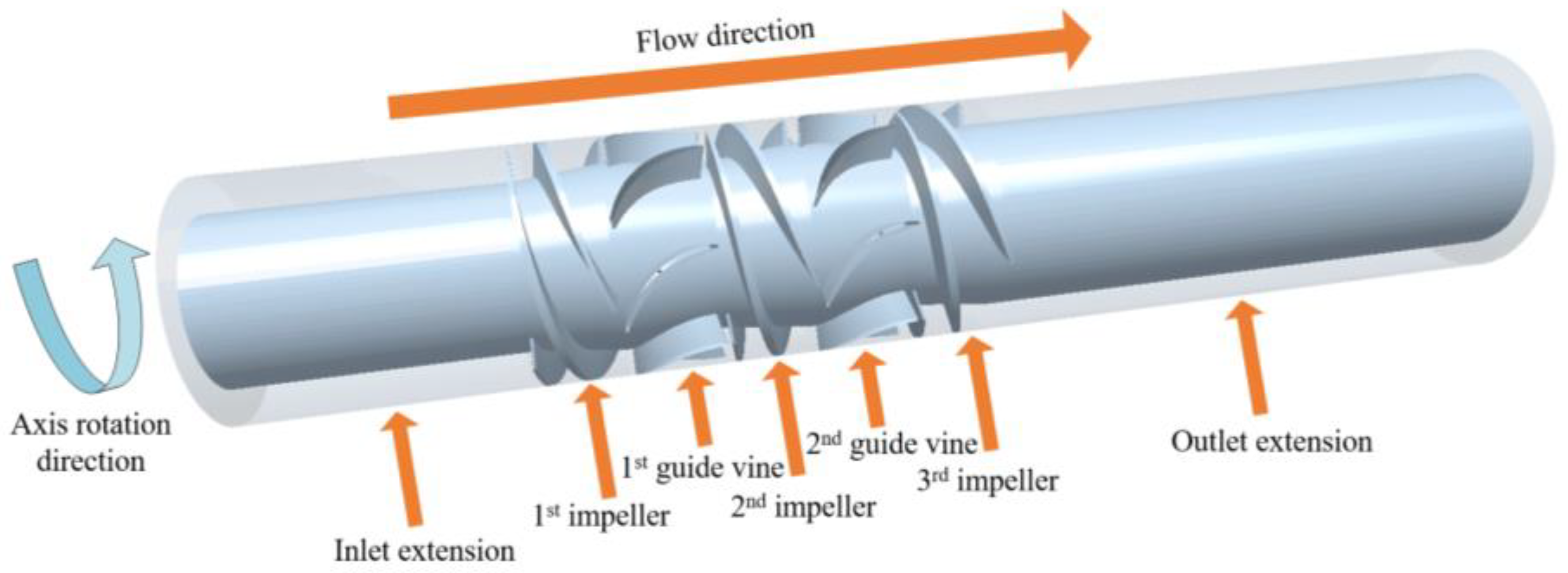
2.1. Calculation Model

The spiral-vane-type multiphase pump was designed with the following key parameters: design flow rate Q = 30 m³/h, design head H = 42 m, operating speed n = 3000 rpm, impeller outer diameter D = 126 mm, three blades per impeller, and three stages. Figure 1 presents the experimental pump prototype, while

Table 1. Main parameters of the spiral-vane-type multiphase transport pump.

Design Parameter	Sign	Value	Unit
number of impeller blades	$Z_1$	3	--
number of guide vane blades	$Z_2$	7	--
the diameter of impeller	$D$	126	mm
hub ratio	$\overline{d}$	0.7	--
the diameter of impeller inlet hub	$D_1$	88.4	mm
the diameter of impeller outlet hub	$D_2$	98.6	mm
axial length of impeller	$e_1$	46.77	mm
axial length of guide vane	$e_2$	51.65	mm
wrap angle of impeller blade	${\alpha }_1$	212	$°$
wrap angle of guide vane blade	${\alpha }_2$	35	$°$

summarizes its detailed geometric dimensions. For ease of research, this study used inlet and outlet pipes to replace the suction and discharge chambers for simulation, and the computational model is presented in Figure 2.

2.2. Mesh Division and Independence Verification

The computational domain was meshed using a hybrid mesh strategy to optimize numerical accuracy and efficiency. The inlet and outlet pipes were meshed with highly adaptable unstructured meshes, while the impellers and guide vanes were divided into hexahedral structured meshes using ANSYS TurboGrid, Available online: https://simtec-europe.com/?gad_source=1&gclid=EAIaIQobChMI9JmCmczwjAMVuaxoCR1LWjbUEAAYASAAEgJkoPD_BwE (accessed on 26 March 2025). Figure 3 displays the mesh of the pressurization unit. A systematic mesh independence study was conducted by evaluating four distinct mesh densities. The pump’s head and hydraulic efficiency served as the indicators of mesh independence, as tabulated in

Table 2. Mesh independence verification.

Scheme	Mesh Number	Head (m)	Efficiency (%)
Scheme 1	2,984,275	33.54	47.78
Scheme 2	3,872,589	34.83	48.27
Scheme 3	4,389,807	36.01	49.56
Scheme 4	4,789,758	36.2	49.39

. The mesh independence study revealed a clear convergence trend in both head and efficiency predictions with increasing mesh density. While in Table 2, Schemes 1 and2 demonstrated notably lower performance values, the results between Scheme 3 (4,389,807 elements) and 4 showed negligible variation (∆H < 0.5%, (∆η < 0.3%), confirming that Scheme 3 provided sufficient mesh density for accurate simulations. Considering computational efficiency and resource limitations, Scheme 3 was selected as the optimal mesh configuration. Furthermore, wall y+ values throughout the computational domain consistently fell within the recommended range of 30–100, satisfying the requirements for standard wall function implementation.

2.3. Mathematical Models and Calculation Method Settings

2.3.1. Continuous Phase Control Equations

The continuous phase was modeled using the Reynolds-averaged Navier–Stokes (RANS) equations, incorporating the continuity equation, momentum conservation equation, and RNG $k-\epsilon$ turbulence model. The RNG $k-\epsilon$ turbulence model was chosen for this calculation because of its superior swirl prediction ability through the improved eddy viscosity formula, more realistic near-wall mesh requirements, and higher computational efficiency under the same hardware conditions.

(1) Continuity equation:

$${\displaystyle \frac{\partial \rho }{\partial t}}\partial +{\displaystyle \frac{\partial }{\partial x_i}}\left(\rho v_i\right)=0,$$

(1)

where $\rho$ represents the fluid density, $t$ denotes time, and $v_i$ is the component of the velocity vector in the direction $i$ of the Cartesian coordinate system.

(2) Momentum conservation equation:

$${\displaystyle \frac{\partial }{\partial t}}\left(\rho v_i\right)+{\displaystyle \frac{\partial }{\partial x_i}}\left(\rho v_i{v}_j\right)=-{\displaystyle \frac{\partial P}{\partial x_i}}+{\displaystyle \frac{\partial {\tau }_{ij}}{\partial x_j}}+\rho g_i+F_i,$$

(2)

where $P$ is the static pressure, $g_i$ and $F_i$ represent gravitational acceleration and external body forces in the direction $i$, respectively, and ${\tau }_{ij}$ denotes the viscous stress tensor.

2.3.2. Discrete Phase Control Equations

In the coupling calculation, the discrete phase mainly solves the force of the particle collision process by the Hertz–Mindlin contact model, uses Newton’s second law to calculate the particle acceleration, and then updates the particle velocity and displacement.

(1) The equation for conservation of momentum:

$$m_i{\displaystyle \frac{d{v}_i}{dt}}={\displaystyle \sum }_j\left(F_{n,ij}+F_{\tau ,ij}\right)+F_{fp,i}+m_{i}g,$$

(3)

where $m_i$ is the mass of particle $i$, $v_i$ is the translational velocity vector, $F_{n,ij}$ is the normal contact force between particle $i$ and particle $j$, $F_{\tau ,ij}$ is the tangential contact forces, $F_{fp,i}$ is the force of the liquid phase relative to particle $i$, and $g$ is gravitational acceleration vector.

(2) The equation for conservation of angular momentum:

$${\displaystyle \frac{d}{dt}}{I}_i{\omega }_i={\displaystyle \sum }_j\left(r_i\times F_{\tau ,ij}+M_i\right),$$

(4)

where $I_i$ is the rotational inertia of particle $i$, ${\omega }_i$ is the angular velocity vector, $M_i$ is the rolling friction torque of particle $i$, and $r_i$ is the contact radius vector of particle $i$.

(3) The contact force between particles (the first term on the right-hand side of Equation (3)). The particle contact forces in the Hertz–Mindlin contact model consist of normal contact forces ($F_{n,ij}$) and tangential contact force ($F_{n,ij}$), as follows:

$$F_{n,ij}=\underset{\mathrm{Elastic} \mathrm{Term}}{\underbrace{{\displaystyle \frac{4}{3}}{E}^{*}\sqrt{R^{*}}{\delta }_n^{3/2}}}{\mathit{n}}_{\mathit{i}\mathit{j}}+\underset{\mathrm{Damping} \mathrm{Term}}{\underbrace{{\gamma }_n\sqrt{6m^{*}{E}^{*}\sqrt{R^{*}{\delta }_n}}}}{\mathit{v}}_{\mathit{n},\mathit{i}\mathit{j}},$$

(5)

where $E^{\mathrm{*}}$ is the effective elastic modulus; $R^{*}$ is the effective radius, ${\displaystyle \frac{1}{R^{*}}}={\displaystyle \frac{1}{R_i}}+{\displaystyle \frac{1}{R_j}}$; ${\delta }_n$ is the normal overlap, ${\delta }_n=R_i+R_j-\left|{\mathit{x}}_{\mathit{i}}-{\mathit{x}}_{\mathit{j}}\right|$; ${\gamma }_n$ is the normal damping coefficient (related to the restitution coefficient $e$), ${\mathsf{\gamma }}_n=-{\displaystyle \frac{2\ln e}{\sqrt{{\ln }^{2}e+{\mathsf{\pi }}^2}}}\sqrt{{\displaystyle \frac{5}{6}}{m}^{*}{E}^{*}\sqrt{R^{*}{\mathsf{\delta }}_n}}$; $m^{*}$ is the effective mass, ${\displaystyle \frac{1}{m^{*}}}={\displaystyle \frac{1}{m_i}}+{\displaystyle \frac{1}{m_j}}$; and $v_{n,ij}$ is the normal relative velocity, $v_{n,ij}=\left(v_j-v_i\right)\cdot n_{ij}$.

$$F_{\tau ,ij}=-\underset{\mathrm{Elastic} \mathrm{Term}}{\underbrace{8G^{*}\sqrt{R^{*}{\delta }_n}{\delta }_{\tau }}}{\mathit{t}}_{\mathit{i}\mathit{j}}+\underset{\mathrm{Damping} \mathrm{Term}}{\underbrace{{\gamma }_{\tau }\sqrt{6m^{*}{G}^{*}\sqrt{R^{*}{\delta }_n}}}}{\mathit{v}}_{\tau ,\mathit{i}\mathit{j}}$$

(6)

where $G^{*}$ is the effective shear modulus, ${\displaystyle \frac{1}{G^{*}}}={\displaystyle \frac{2-{\mathsf{\nu }}_i}{G_i}}+{\displaystyle \frac{2-{\mathsf{\nu }}_j}{G_j}},{ G}_i={\displaystyle \frac{E_i}{2\left(1+{\mathsf{\nu }}_i\right)}}$; ${\mathsf{\delta }}_{\mathsf{\tau }}$ is the tangential overlap, calculated through time integration: ${\mathsf{\delta }}_{\mathsf{\tau }}={\int }_{t_c}{v}_{\mathsf{\tau },ij}\hspace{0.17em}dt$; ${\gamma }_{\tau }$is the tangential damping coefficient, typically set as ${\gamma }_{\tau }={\gamma }_n$; and ${\mathit{v}}_{\tau ,\mathit{i}\mathit{j}}$ is the tangential relative velocity, ${\mathit{v}}_{\tau ,\mathit{i}\mathit{j}}={\mathit{v}}_{\mathit{i}\mathit{j}}-{\mathit{v}}_{\mathit{n},\mathit{i}\mathit{j}}$. Friction limit: $\left|F_{\mathsf{\tau },ij}\right|\le {\mathsf{\mu }}_s\left|F_{n,ij}\right|$. If exceeded, $F_{\tau ,ij}$ is reset to ${\mathsf{\mu }}_s\left|F_{n,ij}\right|$ (${\mathsf{\mu }}_s$ is the static friction coefficient).

(4) The force of the liquid phase relative to the particle (the second term on the right-hand side of Equation (3)). The force of the liquid phase relative to particle ($F_{fp,i}$) includes the drag force, pressure gradient force, virtual mass force, Saffman lift force, and Magnus force, specifically:

$$F_{fp,i}=F_{\mathrm{drag}}+F_{\mathrm{pressure}}+F_{\mathrm{virtual} \mathrm{mass}}+F_{\mathrm{Saffman}}+F_{\mathrm{Magnus}}$$

(7)

The drag force is expressed as follows:

$$F_{\mathrm{drag}}={\displaystyle \frac{1}{2}}{C}_d{\mathsf{\rho }}_f{A}_p\left|u_f-u_p\right|\left(u_f-u_p\right)$$

(8)

where $C_d$ is the drag coefficient, $A_p$ is the projected area of the particle, and $u_f$ is the fluid velocity.

The pressure gradient force is pressed as follows:

$$F_{\mathrm{pressure}}=-V_p\nabla p$$

(9)

where $\nabla p$ is the pressure gradient.

The virtual mass force is pressed as follows:

$$F_{\mathrm{virtual} \mathrm{mass}}=C_{vm}{\mathsf{\rho }}_f{V}_p\left({\displaystyle \frac{d{u}_f}{dt}}-{\displaystyle \frac{d{u}_p}{dt}}\right)$$

(10)

where $C_{vm}$ is the virtual mass.

The Saffman lift force is pressed as follows:

$$F_{\mathrm{Saffman}}=1.615d_p^2\sqrt{{\mathsf{\rho }}_f{\mathsf{\mu }}_f}\left|u_f-u_p\right|{\left(\nabla \times u_f\right)}^{1/2}$$

(11)

where $\nabla \times u_f$ is the vorticity of the fluid.

The Magnus force is pressed as follows:

$$F_{\mathrm{Magnus}}={\displaystyle \frac{1}{2}}{\mathsf{\rho }}_f{A}_p{C}_L\left|u_f-u_p\right|\left(\mathsf{\omega }\times \left(u_f-u_p\right)\right)$$

(12)

where $C_L$ is the lift coefficient, and $\mathsf{\omega }$ is the angular velocity of the particle.

2.3.3. CFD-DEM Coupling

The CFD-DEM coupling methodology employs a transient bidirectional data-exchange mechanism that accounts for interphase mass, momentum, and energy transfer. As depicted in Figure 4, the coupling process is as follows: First, the CFD solver computes the fluid velocity and pressure fields and interpolates the fluid velocity and pressure at the mesh nodes to the particle locations. Based on the local porosity and relative velocity, the Wen–Yu drag force model is used to calculate the drag force exerted by the fluid on the particles, while considering the pressure gradient force, virtual mass force, Saffman lift force, and Magnus force. Subsequently, the DEM solver updates the particle motion state based on these fluid forces and inter-particle contact forces (using the Hertz–Mindlin contact model) and feeds back the particle position and velocity information to the CFD mesh. The local porosity is calculated by statistically determining the particle volume within the mesh, and the reaction force from the particles on the fluid is incorporated into the Navier–Stokes equation as a momentum source term. In terms of time stepping, DEM employs a smaller time step compared to CFD, performing multiple DEM sub-steps within a single CFD time step to ensure numerical stability. Finally, the synchronization of the two-phase data is achieved through iteration.

2.3.4. Calculation Method Settings

In this work, the multiphase system was configured with pure water as the continuous phase and spherical particles as the discrete phase. The interparticle and particle–wall collisions were simulated using the Hertz–Mindlin no-slip contact model. The mechanical properties of the contacting materials were specified as follows: pump material: stainless steel (shear modulus G = 79.8 GPa, Poisson’s ratio $\lambda$ = 0.3) and particle material: rubber (shear modulus G = 21.3 MPa, Poisson’s ratio $\lambda$ = 0.4). The complete set of collision parameters, including restitution coefficients and friction coefficients, are provided in

Table 3. Collision parameters in Hertz–Mindlin contact model.

Collision Coefficient	Particle–Particle	Particle–Wall
Restitution	0.45	0.48
Static friction	0.28	0.16
Rolling friction	0.01	0.01

. This contact model accurately captures the elastic deformation and frictional behavior during particle interactions, which is particularly important for predicting wear patterns in the pump components.

The transient CFD-DEM coupled simulations were conducted using ANSYS Fluent and EDEM software to investigate the multiphase flow characteristics in the model pump. The calculation method is set as follows: (1) Temporal Parameters: The total simulated physical time is 0.9 s. The simulated time step size of the fluid is set to 1×e⁻⁴ s, corresponding to approximately $1°$ of rotation of the impeller. The simulated time step size of the 1 mm particle is set to 5×e⁻⁶ s, which is equivalent to 18% of the Rayleigh time step. (2) The turbulence model adopts the RNG k-epsilon model. (3) The computational domain was divided into two distinct reference frames: a rotating reference frame was applied to the impeller, and a stationary reference frame was used for the guide vane and inlet and outlet pipes. (4) Boundary Conditions: inlet: axially symmetric flow without pre-rotation; outlet: pressure outlet; and walls: no-slip boundary condition, and the standard wall function is used near the wall.

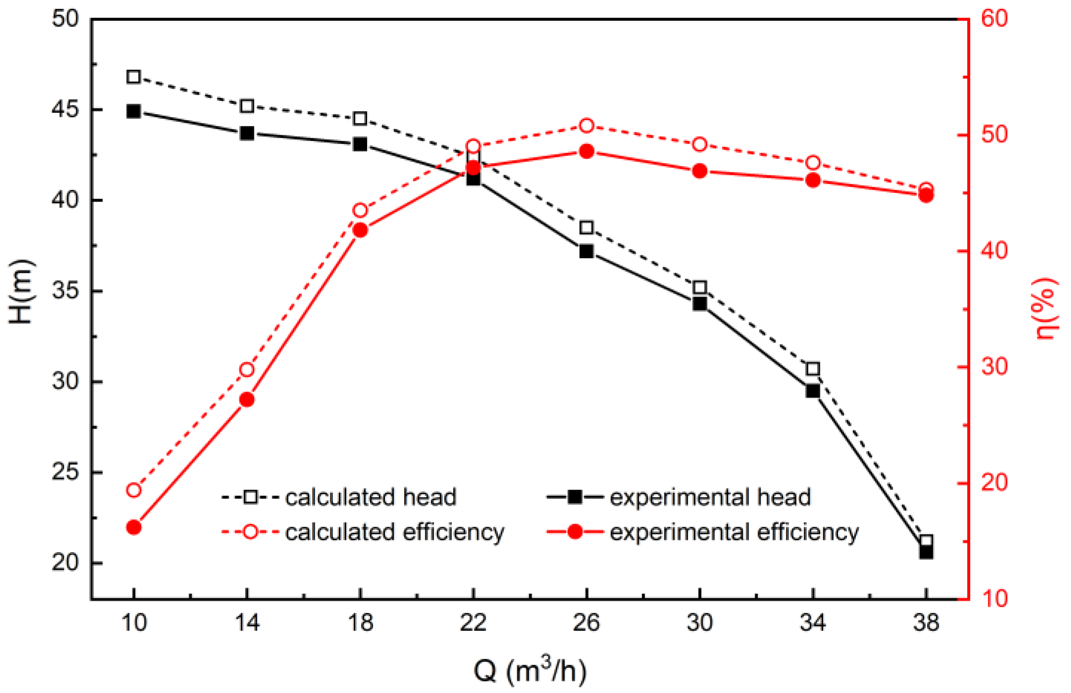
3. Experimental Verification

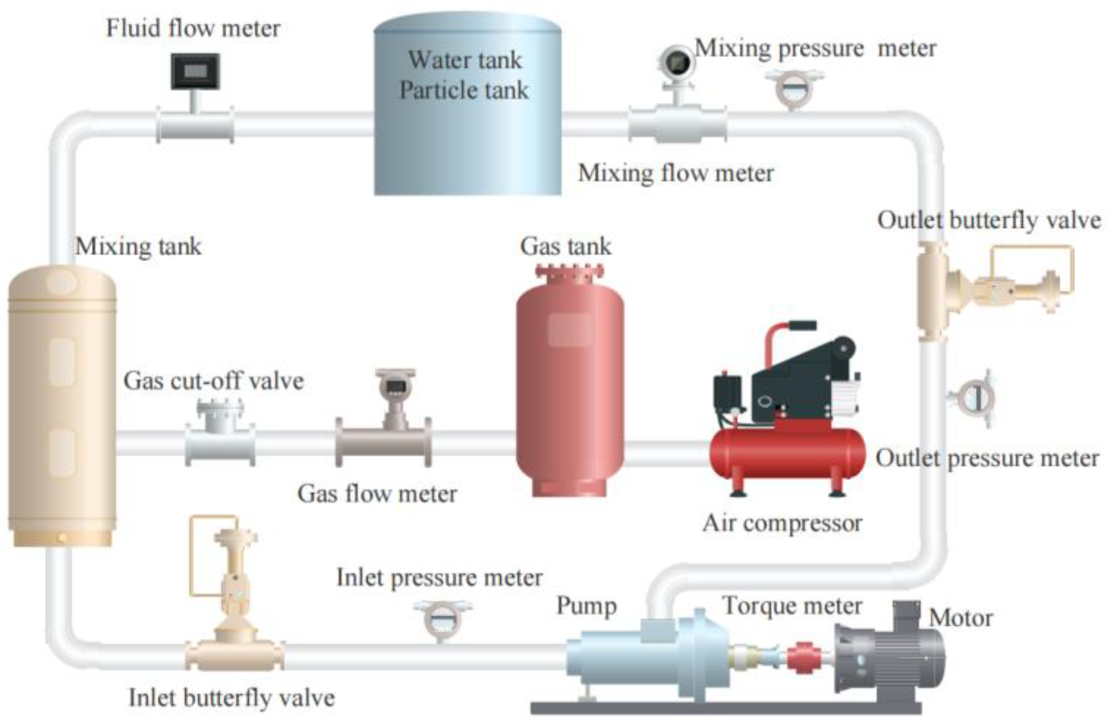
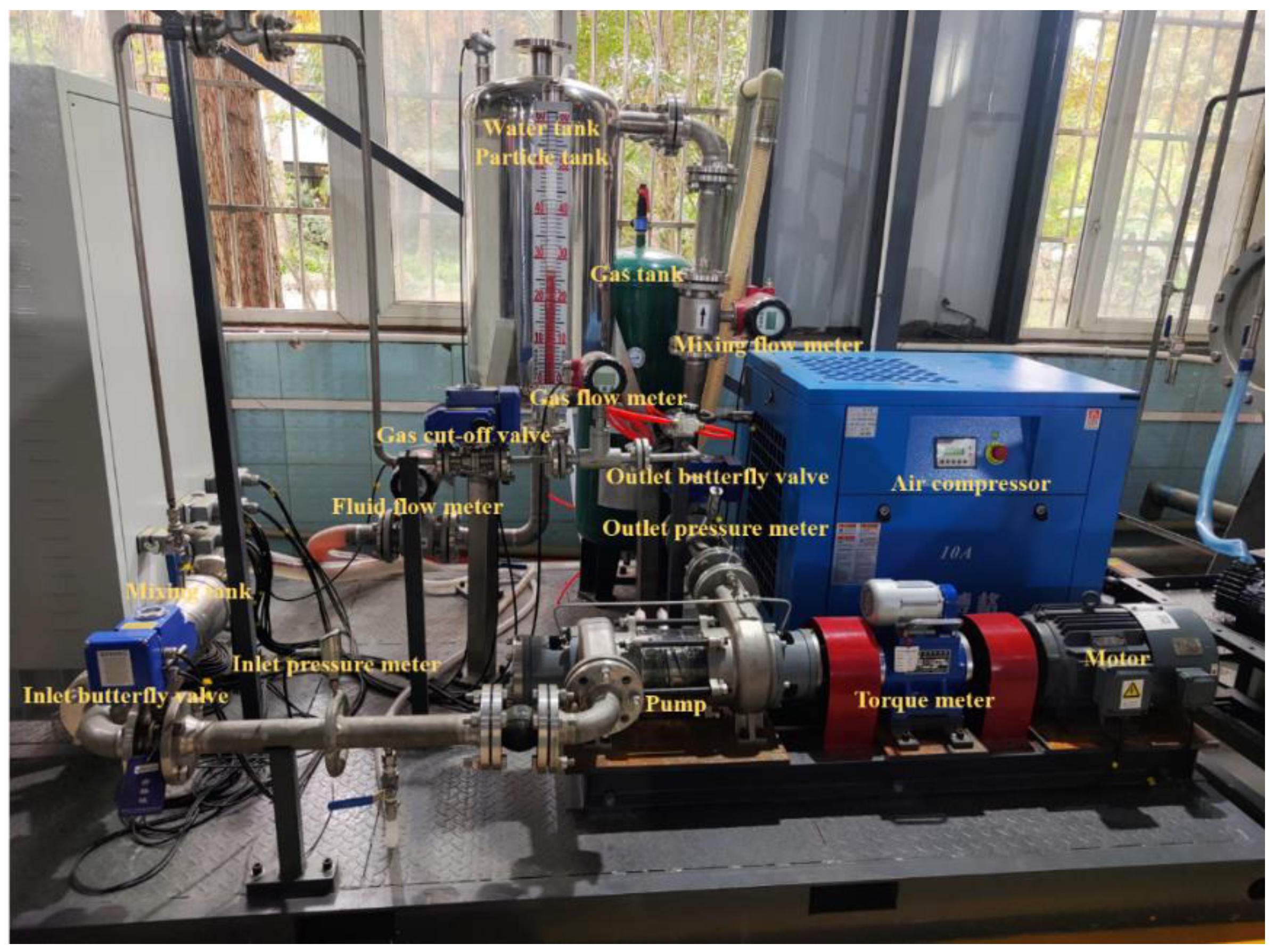
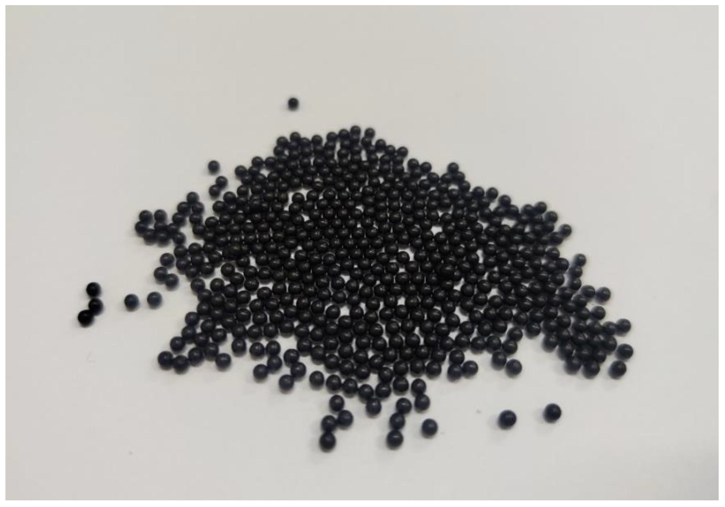
3.1. Experimental Equipment

To validate the numerical simulation results, comprehensive performance tests were conducted on the model pump, complemented by high-speed imaging to capture particle motion. The experimental system (as presented in Figure 5 and Figure 6) comprised three primary subsystems: (1) Hydraulic circuit: A closed-loop system utilizing pure water as the working fluid. Precisely measured rubber particles (d = 2 mm, $\rho$ = 1400 kg/m³, as shown in Figure 7) were introduced through the particle tank. Solid-phase concentration was controlled via gravimetric measurement. (2) Control system: Variable-frequency drive was used for precise pump speed regulation. A flow control valve was used for discharge adjustment. (3) Automated data acquisition system (specifications in

Table 4. Instrument parameters and accuracy.

Test Instrument	Range	Accuracy	Unit
Inlet pressure meter	0–1.6	±0.25%	MPa
Outlet pressure meter	0–1.6	±0.25%	MPa
Fluid flow meter	0–50	±0.25%	m3/h
Torque meter	0–30	±0.25%	Nm

): The measurement equipment included a high-speed camera for particle trajectory visualization, pressure sensor, electromagnetic flow meter, and torque meter.

3.2. Experimental Results

The experimental validation was performed at a fixed particle concentration of 2‰ and rotational speed of 3000 rpm, while varying flow rates to assess the numerical method’s reliability. Using the data acquisition system, we measured the pump’s external characteristics and systematically compared them with numerical predictions. The comparative performance curves presented in Figure 8 reveal agreement between experimental measurements and numerical simulations. Across the operational flow range (10–38 m³/h), the maximum deviation between simulated and experimental results for both head and efficiency remained below 5%. The systematic overprediction (2–4%) in the numerical results primarily stems from unaccounted mechanical losses and leakage effects in the simulation model. These findings confirm that the developed CFD-DEM model reliably captures both the pump’s hydraulic performance and internal particle motion characteristics.

Figure 9 depicts the flow behavior of individual particles within a single passage of the first-stage guide vane, as observed through high-speed imaging (with experimental results on the left and CFD-DEM coupled simulation results on the right). As shown in the figure, the particles are initially spaced apart when they enter the first-stage guide vane. Over time, the distance between them progressively narrows until a uniform spacing is achieved, suggesting that the particle velocity gradually slows down and stabilizes upon entering the first-stage guide vane. Furthermore, the particle motion patterns captured by the CFD-DEM simulation closely resemble those observed experimentally, confirming that the CFD-DEM model accurately reflects the particle trajectories and validating the reliability of the numerical results.

4. Analysis of Numerical Results

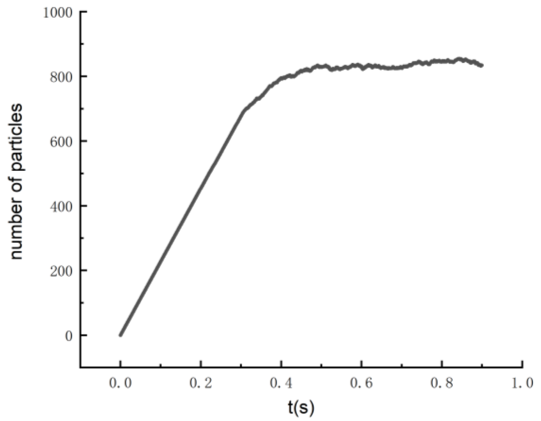
4.1. Time Independence Analysis

To ensure the stability of particle motion within the pump and the reliability of the analysis, an independence analysis of the simulation time was conducted. Figure 10 presents the temporal evolution of particle distribution characteristics obtained through periodic sampling within the pump. Significant particle count fluctuations are observed during the initial 0.4 s period, corresponding to incomplete particle circulation cycles. Beyond this transitional phase, the particle population demonstrates progressive stabilization. Taking into account computational time and other factors, the simulation data from 0.4 to 0.9 s were selected for further analysis. The data within this time frame exhibit a certain degree of stability and can be used to analyze the particles motion characteristics within the spiral-vane-type multiphase pump for different diameters.

4.2. Analysis of Single-Particle Flow in the Pump

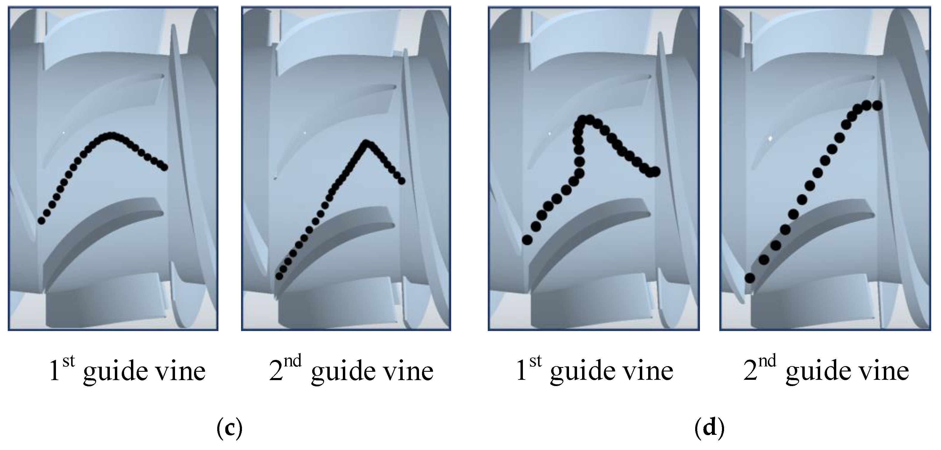
4.2.1. The Particle Trajectories Under Different Diameters in the Guide Vanes

Figure 11 displays the absolute motion trajectories of particles under different diameters in guide vanes. The single particle trajectory in the guide vanes in the DEM numerical calculation results is tracked, the position information of a single particle at different times is extracted to fit into a spatial trajectory, and the absolute motion trajectory of the particle is obtained. Here, the blade below each guide vane channel is defined as the No. 1 blade, and the upper blade is defined as the No. 2 blade.

As shown in Figure 11a, the 0.5 mm particle enters the first stage guide vane close to the suction side on the No. 1 blade, moves along the suction side to the middle position of the blade, then move towards the center of the flow passage, and finally enters second-stage impeller. Then, the particle enters the second guide vane along the pressure side on the No. 2 blade and moves to the blade outlet along the pressure side. For smaller diameter particles, the flow following is better, so it can better adapt to the changes of the blade surface and maintain a stable motion trajectory.

As shown in Figure 11b, the 1 mm particle enters the first stage guide vane from the suction side on the No. 1 blade, begins to move to the center of the flow passage, and finally enters second-stage impeller. The particle then enters the second stage guide vane and moves to the guide vane outlet along the center of the flow passage.

From Figure 11c, the 1.5 mm particle enters the first stage guide vane along the center of the flow passage and moves towards the pressure side on the No. 2 blade. When it moves to the vicinity of the pressure surface in the middle of the No. 2 blade, it begins to deviate from the pressure surface until the outlet of the flow channel, which may be caused by the vortex flow near the outlet of the pressure surface of the No. 2 blade. Subsequently, the particle entered the second stage guide vanes close to the suction surface at the inlet of the No. 1 blade, and moved towards the center of the flow passage. When it moved to the vicinity of the No. 2 blade outlet on the pressure side, it also began to deviate from the pressure side until the outlet of the impeller flow passage.

From Figure 11d, the 2 mm particle flows into primary guide vanes from the No. 1 blade inlet on the suction side along the center of the flow passage. When particle moves to the center position, it begins to move directly to the pressure side on the No. 2 blade under the influence of the vortex. After it collides with the center of the pressure side, it then moves along the center of the flow passage to the impeller outlet. At this time, the particle flows into the second guide vane near the suction side on the No. 1 blade. Then, it moves towards the pressure side of the No. 2 blade until flowing out the blade outlet. For larger diameter particles (2 mm), due to their high inertia and poor flow following, the path of the particle in the impeller and guide vane region usually exhibits a large deviation, often accompanied by a collision with the wall.

From Figure 11, the particle spacing with different sizes is large when entering the guide vane. As time goes on, the spacing of the particles decreases continuously until it becomes uniform, indicating that after the particles flow into the first guide vane, their velocity progressively decreases and tends to be stable. The wrap angle for the motion trajectory with the 0.5 mm and 1 mm particles is smaller, while the wrap angle for the motion trajectory with 1.5 mm and 2 mm particles is larger, and there is a collision with the wall. This is due to the fact that the coarse particles may attain more kinetic energy after passing through the impeller, and their flow following is worse.

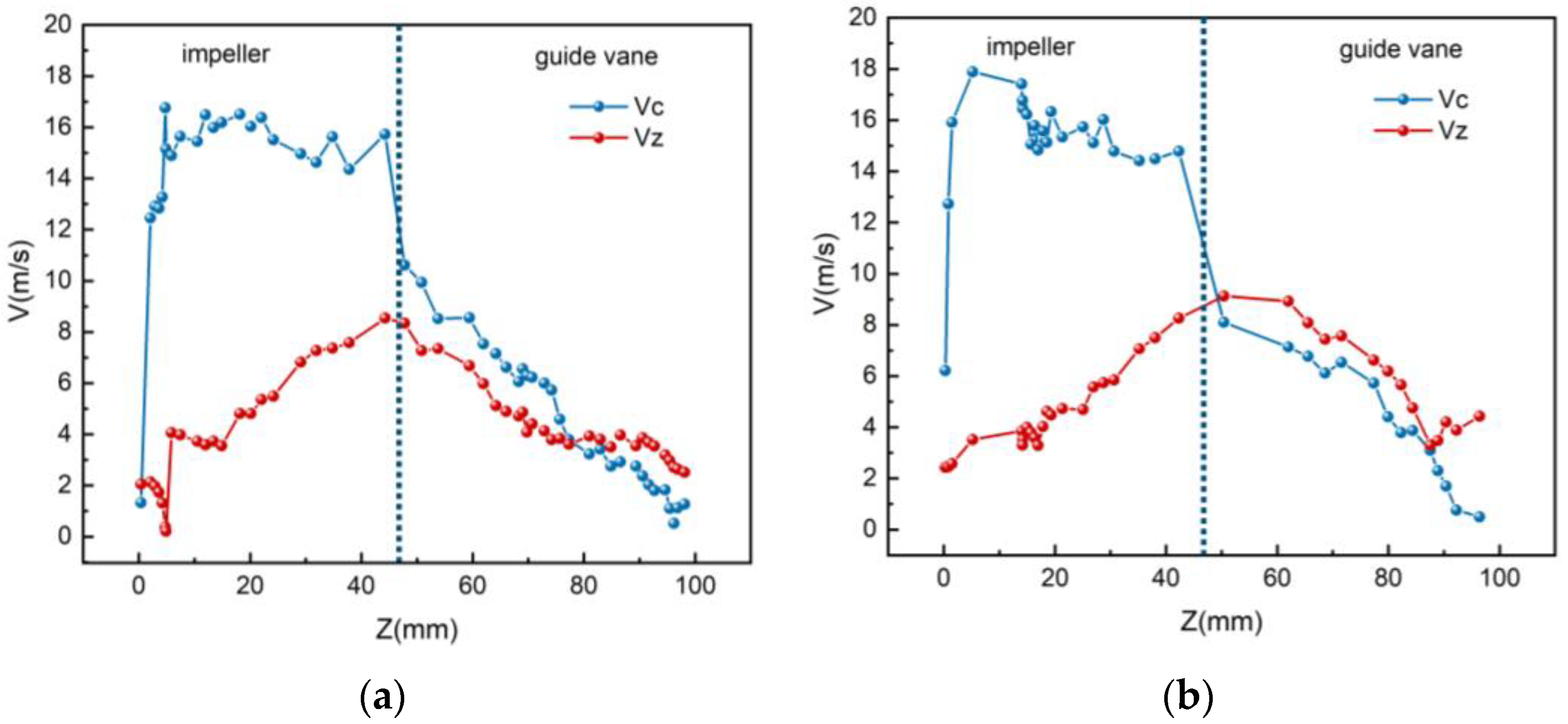
4.2.2. The Velocity Change of the Particles with Different Diameters in the Pressurization Unit

The velocity evolution of the 0.5 mm particles within the pressurization units is presented in Figure 12. In the figure, the left side of the dotted line represents the impeller region, while the right side corresponds to the guide vane region. Vc represents the circumferential velocity of the particle, and Vz represents the axial velocity of the particle. As Figure 12a shows, upon entering first-stage impeller, the 0.5 mm particles experience blade-leading-edge collisions, resulting in a rapid circumferential velocity increase to approximately 15 m/s due to impeller’s high-speed rotation. The axial velocity of the particles fluctuates slightly because of the impact of the rotor–stator interaction when it just enters the first stage impeller, and then begins to increase slowly, reaching a maximum value of 7.39 m/s near the impeller blade outlet. Once the particles flow into the first guide vane, the circumferential velocity decreases sharply from 16.05 m/s to 10.68 m/s at the guide vane inlet because of the separation from the high-speed rotating impeller blade. Now it decreases gradually along the flow passage of the guide vanes. The acceleration process of the particles in the impeller reflects the strong force exerted by the impeller blades on the particles, causing a rapid increase in the circumferential velocity of the particles. Particularly, after the particles enter the impeller, due to the high-speed rotation of the impeller blades, the tangential acceleration of the particles is significant, allowing them to quickly adapt to the rotating flow field and reach a stable velocity. Simultaneously, the axial velocity decreases slowly along the guide vane channel. As shown in Figure 12b, the particle velocity in the secondary pressurization unit also shows a similar law, but the maximum circumferential velocity and axial velocity in the secondary pressurization unit are higher than those in the primary pressurization unit.

The velocity evolution of the 1 mm particles in the pressurization stage is quantitatively demonstrated in Figure 13. In Figure 13a, when the particle just enters the first-stage impeller, the circumferential velocity rises sharply from 1.32 m/s to 12.45 m/s. After that, it stabilizes at about 15 m/s. The axial velocity also fluctuates slightly near the impeller inlet, and then increases slowly to 8.34 m/s. When the particle flows into the guide vane flow passage, the circumferential velocity first plummets by 5.12 m/s. After that, it gradually decreases, while the axial velocity also begins to decrease slowly, and the slope of the decrease of the circumferential velocity is larger than that of the axial velocity. In Figure 13b, when the 0.5 mm particle enters second-stage impeller, the velocity variation law of the 0.5 mm particle is similar to that of the first one. When entering the second guide vane, the axial velocity is bigger than the circumferential velocity, which is consistent with the trajectory of the 0.5 mm particle entering the second guide vane along a slope below 45°, as displayed in Figure 11b.

The velocity evolution of the 1.5 mm particles within the pressurization units is presented in Figure 14. It can be seen from Figure 14a, when the 1.5 mm particle just enters first-stage impeller, the circumferential velocity rises sharply from 1.13 m/s to 8.03 m/s. Then it stabilizes at about 16 m/s. Due to the large inertia of the particles, the 1.5 mm particle can adapt to the high-speed rotation of the impeller better than the small particles, and achieve a higher circumferential speed. The axial velocity also fluctuates slightly near the impeller inlet, and then increases slowly to 7.35 m/s. The circumferential velocity begins to decrease sharply, and the axial velocity also begins to decrease slowly when the particle flows into the first guide vane. When it drops to the center of the guide vane, then the two begin to increase. This is because the guide vane outlet vortex significantly influences particle motion, which also corresponds to the trajectory of the 1.5 mm particle in the first guide vane in Figure 11c. For Figure 14b, the velocity change for the 1.5 mm particle size in second-stage impeller is close to that in first-stage impeller. Upon entering the second guide vane, 1.5 mm particle exhibit progressive deceleration in both circumferential and axial velocity components. When it moves near the guide vane outlet, both forces begin to increase, which is also because of the influence of the vortex flow at the guide vane outlet.

The velocity evolution of the 2 mm particles within the pressurization units is presented in Figure 15. For Figure 15a, when the 2 mm particle just enters first-stage impeller, the circumferential velocity rises sharply from 8.31 m/s to 15.69 m/s, and then stabilizes at about 15 m/s. The axial velocity did not increase significantly near the impeller inlet, and began to increase gradually in the second part of the impeller passage, reaching a maximum value of 8.37 m/s at the impeller outlet. After entering first-stage guide vine, the circumferential velocity and the axial velocity begin to decline sharply. In the center of the guide vane passage, the particles and the pressure side on the guide vane blade are about to collide. The circumferential velocity is reduced to 0 m/s. The axial velocity is negative. And then, the circumferential velocity and the axial velocity begin to increase, and then stabilize at about 2 m/s. The eddy current in the fluid changes the trajectory of the particles and exerts a reverse force on the particles at a specific position, resulting in a change in the velocity direction of the particles. From Figure 15b, when the 2 mm particle just enters the second stage impeller, the circumferential velocity rises sharply from 8.31 m/s to 15.69 m/s, and then stabilizes at about 15 m/s. The axial velocity fluctuates slightly around 2 m/s at the impeller inlet, and then begins to increase gradually. After entering the second guide vane, and the circumferential velocity first begins to drop suddenly. When it reaches the center of the guide vane, and the circumferential velocity almost coincides with the axial velocity, which is also reflected in the 45° trajectory of the 2 mm particle in the second half of the second stage guide vane in Figure 11d.

From Figure 12, Figure 13, Figure 14 and Figure 15, it can be observed that the velocity variations for all four particle sizes within the pressurization unit follow similar patterns. First, the particles flow into the impeller, and then the circumferential velocity increases sharply after the collision with the high-speed rotating impeller blade, and then stabilizes at about 15 m/s, which corresponds to the linear velocity for the different particles at 3000 rpm. When the particles just enter the guide vane, the circumferential velocity drops sharply after the particles are separated from the impeller area, and then gradually decreases within the guide vane channel. The axial velocity may fluctuate slightly in the impeller inlet area because of the impact of the rotor–stator interaction, then, in the impeller flow passage, it gradually rises, reaches the highest value at the impeller outlet, and begins to decrease gradually after entering the guide vane.

4.3. The Distribution of the Particles in the Pressurization Unit

Figure 16 displays the volume fraction distribution for the different particles in the compression unit. From Figure 16, the volume fraction of the four particle sizes in guide vanes is greater than that in impellers. The volume fraction of different particles in the impeller is not very different, and the volume fraction in the guide vane is quite different. Within the diameter of 1.5 mm, particle volume fraction in the guide vane shows a positive correlation with particle diameter.

4.4. Collisions Between Particles and Walls

4.4.1. Collision Distribution of the Particles with Different Diameters in the Pressurization Unit

Figure 17 displays the distribution of particle collision with the different particle sizes in each pressurization unit. Figure 17 demonstrates that the particles tend to collide on the impeller wall. Then, the proportion of the collision on the guide vane wall is very small. With the growth of particle diameter size, the collision ratio on the guide vane wall increases. This trend can be explained by the increased inertia of larger particles, which causes them to have less effective interaction with the fluid and thus increases their likelihood of contacting the guide vane wall. It can also be seen that the collision on the first guide vane is more than that on the second guide vane. The reason is as follows: When particles just enter the second guide vane, they pass through the rectification for the first guide vane. The angle of guide vane outlet is 90°. Therefore, the particles leave the first guide vane basically, and enter second-stage impeller vertically at an angle of 90°. The trajectory is better, so the number of collisions is less.

4.4.2. Particle–Wall Contact Forces at Different Diameters

Figure 18 shows the particle–wall contact force under the four particle sizes in each pressurization unit. The contact force of the four particle sizes in the impellers at all levels is greater than that in the guide vanes. This finding is consistent with the collision distribution shown in Figure 17, confirming the greater intensity of particle–wall interactions in the impeller regions compared to the guide vanes.

In the impeller, below the 1.5 mm particle size, with the growth of particle size, the contact force between the particles and impeller wall growths gradually, but at 2 mm particle size, the contact force among particles and impeller wall decreases. This is because at the same mass concentration, the number of particles with a 2 mm particle size declines, thus the probability of collision with impeller wall decreases.

5. Conclusions

The CFD-DEM coupling technique is adopted to reveal the distribution and motion characteristics for different particle sizes in the spiral-vane-type multiphase pump. The reliability of the method is verified with the experimental results. The main conclusions are as follows:

• When the particles enter the guide vanes, the initial spacing between particles is relatively large. Over time, the spacing gradually decreases and becomes uniform, indicating that the particle speed decreases and eventually stabilizes after entering the first stage of the guide vanes. The trajectory angles of the 0.5 mm and 1 mm particles are smaller, while those of 1.5 mm and 2 mm particles are larger and more prone to collision with the wall. This suggests that the coarser particles gain more kinetic energy after passing through the impeller and exhibit worse flow-following behavior.
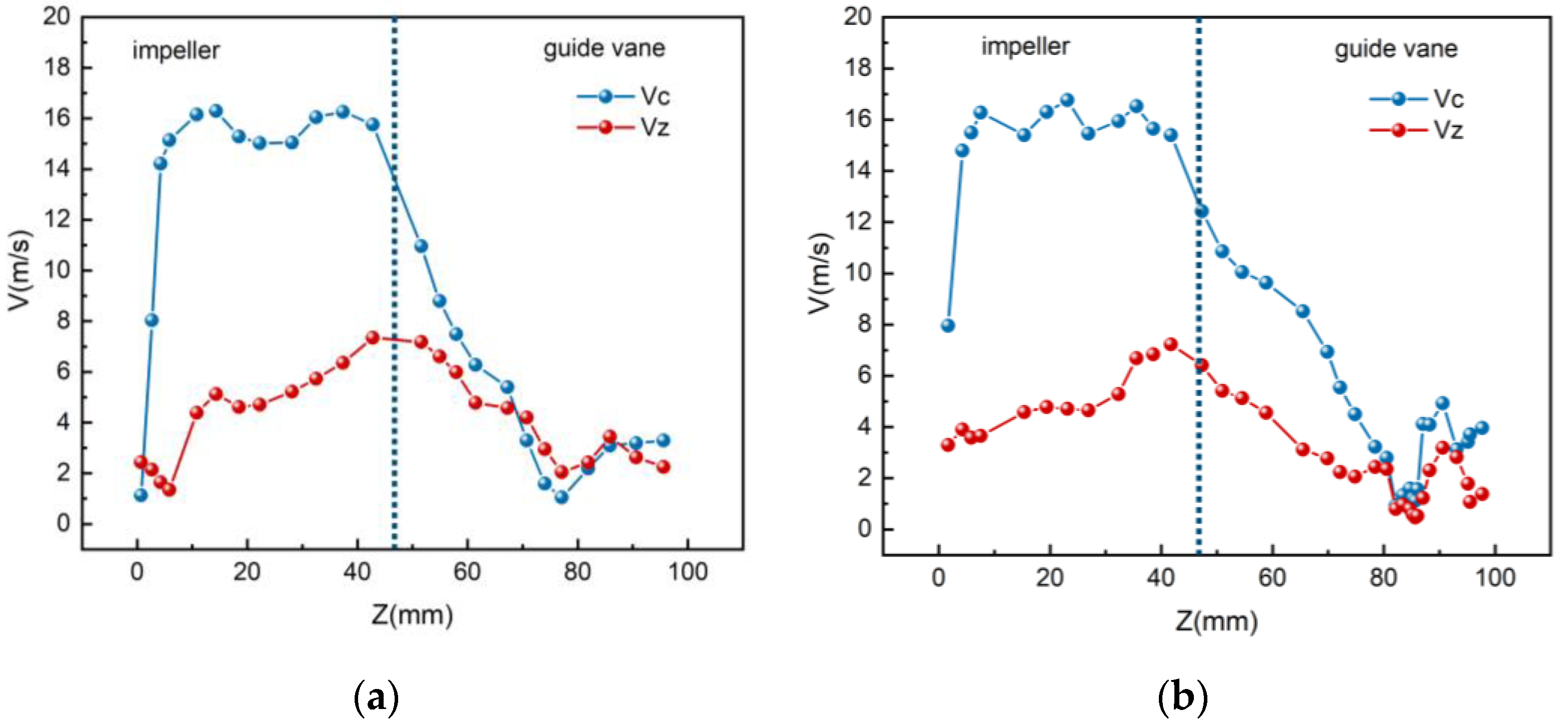
• The velocity variation patterns of the four different diameter particles in the pressurization unit are similar. After entering the impeller, the particles’ circumferential velocity increases sharply and stabilizes around 15 m/s. Upon leaving the impeller, the circumferential velocity drops sharply, and it gradually decreases after entering the guide vanes. The axial velocity experiences small fluctuations due to dynamic–static interference at the impeller inlet, then increases gradually, reaching its maximum value at the impeller exit, and subsequently decreases after entering the guide vanes.
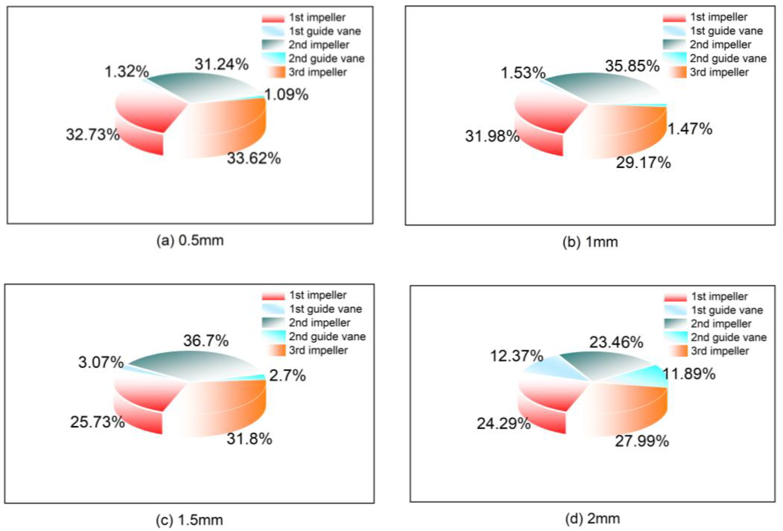
• The volumetric fraction of the four particle diameters inside the guide vanes is larger than that inside the impeller, with a larger discrepancy in the volumetric fraction within the guide vanes. The volumetric fraction of the particles with a diameter of 1.5 mm or less increases as the particle diameter increases.
• Particles collide more frequently with the impeller wall than with the guide vane wall. As the particle diameter increases, the proportion of collisions with the guide vane wall also increases. For particles of 1.5 mm and smaller, increasing the particle diameter leads to more severe collisions with the impeller wall, but for 2 mm particles, the collision probability decreases due to the reduced number of particles. Inside the guide vanes, as the particle diameter increases, the contact force between the particles and the guide vane wall gradually increases.

References

1. Suh, J.-W.; Kim, J.W.; Choi, Y.-S.; Kim, J.-H.; Joo, W.-G.; Lee, K.-Y. Development of numerical Eulerian-Eulerian models for simulating multiphase pumps. J. Pet. Sci. Eng. 2018, 162, 588–601. [Google Scholar] [CrossRef]
2. Kim, J.-H.; Lee, H.-C.; Kim, J.-H.; Choi, Y.-S.; Yoon, J.-Y.; Yoo, I.-S.; Choi, W.-C. Improvement of hydrodynamic performance of a multiphase pump using design of experiment techniques. J. Fluids Eng. 2015, 137, 081301. [Google Scholar] [CrossRef]
3. Mehta, M.; Kadambi, J.R.; Sastry, S.; Sankovic, J.; Wernet, M.; Addie, G.; Visintainer, R. Study of particulate flow in the impeller of a slurry pump using PIV. In Proceedings of the Summer Conference, Proceedings of the Heat Transfer, Charlotte, NA, USA, 11–15 July 2004; Volume 46903, pp. 489–499. [Google Scholar]
4. Cader, T.; Masbernat, O.; Roco, M.C. LDV measurements in a centrifugal slurry pump: Water and dilute slurry flows. J. Fluids Eng. 1992, 114, 606–615. [Google Scholar] [CrossRef]
5. Shi, B.; Wei, J.; Zhang, Y. Phase discrimination and a high accuracy algorithm for PIV image processing of particle–fluid two-phase flow inside high-speed rotating centrifugal slurry pump. Flow Meas. Instrum. 2015, 45, 93–104. [Google Scholar] [CrossRef]
6. Shi, B.; Wei, J.; Zhang, Y. A novel experimental facility for measuring internal flow of Solid-liquid two-phase flow in a centrifugal pump by PIV. Int. J. Multiph. Flow 2017, 89, 266–276. [Google Scholar] [CrossRef]
7. Li, Y.; Zhang, H.; Lin, Z.; He, Z.; Xiang, J.; Su, X. Relationship between wear formation and large-particle motion in a pipe bend. R. Soc. Open Sci. 2019, 6, 181254. [Google Scholar] [CrossRef]
8. Wang, K.; Hu, J.; Liu, H.; Zhang, Z.; Zou, L.; Lu, Z. Research on the deposition characteristics of integrated prefabricated pumping station. Symmetry 2020, 12, 760. [Google Scholar] [CrossRef]
9. Kadambi, J.R.; Charoenngam, P.; Subramanian, A.; Wernet, M.P.; Sankovic, J.M.; Addie, G.; Courtwright, R. Investigations of particle velocities in a slurry pump using PIV: Part 1, the tongue and adjacent channel flow. J. Energy Resour. Technol. 2004, 126, 271–278. [Google Scholar] [CrossRef]
10. Wang, Y.; Wang, X.; Chen, J.; Li, G.; Liu, H.; Xiong, W. Numerical simulation of the influence of mixed sand on erosion characteristics of centrifugal pump. Eng. Comput. 2022, 39, 2053–2080. [Google Scholar] [CrossRef]
11. Jiang, L.; Bai, L.; Xue, P.; Peng, G.; Zhou, L. Two-way coupling simulation of solid-liquid two-phase flow and wear experiments in a slurry pump. J. Mar. Sci. Eng. 2022, 10, 57. [Google Scholar] [CrossRef]
12. Hong, S.; Hu, X. Research on wear characteristics and experiment on internal through-passage components for a new type of deep-sea mining pump. Processes 2021, 10, 58. [Google Scholar] [CrossRef]
13. Askaripour, H.; Dehkordi, A.M. Simulation of 3D freely bubbling gas–solid fluidized beds using various drag models: TFM approach. Chem. Eng. Res. Des. 2015, 100, 377–390. [Google Scholar] [CrossRef]
14. Shi, W.; Hou, Y.; Zhou, L.; Li, Y.; Xue, S. Numerical simulation and test of performance of deep-well centrifugal pumps with different stages. J. Drain. Irrig. Mach. Eng. 2019, 37, 562–567. [Google Scholar]
15. Araoye, A.A.; Badr, H.M.; Ahmed, W.H.; Habib, M.A.; Alsarkhi, A. Erosion of a multistage orifice due to liquid-solid flow. Wear 2017, 390, 270–282. [Google Scholar] [CrossRef]
16. Cundall, P.A.; Strack, O.D.L. A discrete numerical model for granular assemblies. Géotechnique 1979, 29, 47–65. [Google Scholar] [CrossRef]
17. Deng, L.; Lu, H.; Liu, S.; Hu, Q.; Yang, J.; Kang, Y.; Sun, P. Particle anti-accumulation design at impeller suction of deep-sea mining pump and evaluation by CFD-DEM simulation. Ocean. Eng. 2023, 279, 114598. [Google Scholar] [CrossRef]
18. Zhao, R.-J.; Zhao, Y.-L.; Zhang, D.-S.; Li, Y.; Geng, L.-L. Numerical investigation of the characteristics of erosion in a centrifugal pump for transporting dilute particle-laden flows. J. Mar. Sci. Eng. 2021, 9, 961. [Google Scholar] [CrossRef]
19. Tang, C.; Yang, Y.-C.; Liu, P.-Z.; Kim, Y.-J. Prediction of abrasive and impact wear due to multi-shaped particles in a centrifugal pump via CFD-DEM coupling method. Energies 2021, 14, 2391. [Google Scholar] [CrossRef]
20. Chen, J.; Chen, X.; Li, W.; Zheng, Y.; Li, Y. Research on Two-Phase Flow and Wear of Inlet Pipe Induced by Fluid Prewhirl in a Centrifugal Pump. J. Mar. Sci. Eng. 2024, 12, 950. [Google Scholar] [CrossRef]
21. Jiang, S.; Zhang, W.; Chen, X.; Cao, G.; Tan, Y.; Xiao, X.; Liu, S.; Yu, Q.; Tong, Z. CFD-DEM simulation research on optimization of spatial attitude of concrete pumping boom based on evaluation of minimum pressure loss. Powder Technol. 2022, 403, 117365. [Google Scholar] [CrossRef]
22. Wang, R.; Guan, Y.; Jin, X.; Tang, Z.; Zhu, Z.; Su, X. Impact of Particle Sizes on Flow Characteristics of Slurry Pump for Deep-Sea Mining. Shock. Vib. 2021, 1, 6684944. [Google Scholar] [CrossRef]
23. Li, Y.; Liu, D.; Cui, B.; Lin, Z.; Zheng, Y.; Ishnazarov, O. Studying particle transport characteristics in centrifugal pumps under external vibration using CFD-DEM simulation. Ocean. Eng. 2024, 301, 117538. [Google Scholar] [CrossRef]
24. Gao, X.; Shi, W.; Shi, Y.; Chang, H.; Zhao, T. DEM-CFD simulation and experiments on the flow characteristics of particles in vortex pumps. Water 2020, 12, 2444. [Google Scholar] [CrossRef]
25. Deng, L.; Hu, Q.; Chen, J.; Kang, Y.; Liu, S. Particle distribution and motion in six-stage centrifugal pump by means of slurry experiment and CFD-DEM simulation. J. Mar. Sci. Eng. 2021, 9, 716. [Google Scholar] [CrossRef]
26. Su, X.; Tang, Z.; Li, Y.; Zhu, Z.; Mianowicz, K.; Balaz, P. Research of particle motion in a two-stage slurry transport pump for deep-ocean mining by the CFD-DEM method. Energies 2020, 13, 6711. [Google Scholar] [CrossRef]
27. Jiang, S.; Chen, X.; Cao, G.; Tan, Y.; Xiao, X.; Zhou, Y.; Liu, S.; Tong, Z.; Wu, Y. Optimization of fresh concrete pumping pressure loss with CFD-DEM approach. Constr. Build. Mater. 2021, 276, 122204. [Google Scholar] [CrossRef]
28. Huang, S.; Su, X.; Qiu, G. Transient numerical simulation for solid-liquid flow in a centrifugal pump by DEM-CFD coupling. Eng. Appl. Comput. Fluid Mech. 2015, 9, 411–418. [Google Scholar] [CrossRef]
29. Zhu, Z.; Sun, J.; Lin, Z.; Jin, Y.; Li, Y. Characterization of the ellipsoidal particle motion in a two-stage lifting pump using CFD-DEM method. Comput. Part. Mech. 2024, 1–16. [Google Scholar] [CrossRef]
Figure 1. A photograph of the test pump.
Jmse 13 00845 g001
Figure 2. Spiral-vane-type multiphase transport pump model.
Jmse 13 00845 g002
Figure 3. Mesh of the pressurization unit: (a) impeller and (b) guide vane.
Jmse 13 00845 g003
Figure 4. CFD-DEM coupling.
Jmse 13 00845 g004
Figure 5. Schematic of multiphase transportation equipment system.
Jmse 13 00845 g005
Figure 6. Multiphase transportation equipment system.
Jmse 13 00845 g006
Figure 7. 2 mm diameter spherical rubber particle.
Jmse 13 00845 g007
Figure 8. Comparison of pump performance characteristics.
Jmse 13 00845 g008
Figure 9. Single-particle absolute-motion trajectory comparison: the left side is the experiment, the right side is CFD-DEM.
Jmse 13 00845 g009
Figure 10. Time independence analysis.
Jmse 13 00845 g010
Figure 11. Trajectory of the particles with different diameters in the guide vanes: (a) 0.5 mm; (b) 1 mm; (c) 1.5 mm; and (d) 2 mm.
Jmse 13 00845 g011aJmse 13 00845 g011b
Figure 12. Change in the particle velocity of the 0.5 mm particle: (a) the primary pressurization unit and (b) the secondary pressurization unit.
Jmse 13 00845 g012
Figure 13. Change in the particle velocity of the 1 mm particle: (a) the primary pressurization unit and (b) the secondary pressurization unit.
Jmse 13 00845 g013
Figure 14. Change in the particle velocity of the 1.5 mm particle: (a) the primary pressurization unit and (b) the secondary pressurization unit.
Jmse 13 00845 g014
Figure 15. Change in the particle velocity of the 2 mm particle: (a) the primary pressurization unit and (b) the secondary pressurization unit.
Jmse 13 00845 g015
Figure 16. The volume fraction distribution of the particles with different diameters in the pressurization unit.
Jmse 13 00845 g016
Figure 17. Collision distribution of the particles with different diameters.
Jmse 13 00845 g017
Figure 18. Particle–wall contact force.
Jmse 13 00845 g018