Abstract
In the context of global climate change and accelerated urbanization, coastal cities face severe threats from storm surges, and accurately predicting coastal water level changes during storm surges has become a core technological demand for disaster prevention and reduction. Storm surges are caused by atmospheric pressure and wind conditions, and their destructive power is closely related to the morphology of the coastline. Traditional tide level prediction models often face difficulties in boundary condition parameterization. Tide level changes result from the combined effect of various complex processes. In past prediction studies, harmonic analysis and numerical simulations have dominated, each with their own limitations. Although machine learning applications in tide prediction have garnered attention, issues such as data inconsistency or missing data still exist. The physical–data fusion approach aims to overcome the limitations of single methods but still faces some challenges. This paper proposes a Deep-Numerical-Reinforcement learning fusion prediction model (DNR), which adopts ensemble learning. First, deep learning models and the numerical model Finite-Volume Coastal Ocean Model (FVCOM) are used to predict tide levels at different tide stations, and then a fusion approach based on the improved reinforcement learning model DDPG_dual is applied for model assimilation. This reinforcement learning fusion model includes a module specifically designed to handle tide extreme points. In the case of the Typhoon Mangkhut storm surge, the DNR model achieved the best results for tide level predictions at six tide stations in the South China Sea.
1. Introduction
In recent decades, coastal cities have rapidly developed into thriving centers of population and economic activity, benefiting from convenient ports, rich tourism resources, and concentrated industries. However, with global climate change intensifying and urbanization accelerating, these coastal regions have become increasingly vulnerable to storm surges. When powerful weather events, such as typhoons or hurricanes, coincide with astronomical high tides, the resulting surge can cause extensive flooding, infrastructure damage, and heavy losses of life and property. History provides numerous examples of the destruction caused by such events. In 1953, a devastating flood submerged a vast area of land in the Netherlands, killing 1836 people [1]. Similarly, when Hurricane Katrina struck New Orleans in 2005, flooding severely breached levees, killing over 1400 people and inflicting economic damage exceeding USD 125 billion in 2005 dollars [2]. Super Typhoon Haiyan in 2013 left around 6000 dead in the Philippines, with economic losses reaching approximately USD 802 billion in 2013 dollars [3]. These tragic events highlight the critical importance of accurately forecasting coastal water levels during storm surges to improve disaster preparedness and response efforts.
As sea levels rise and storm intensity increases, coastal regions face heightened risks from storm surges. Reliable prediction of coastal water levels has thus emerged as a crucial requirement for disaster prevention and mitigation efforts. Accurate forecasts offer critical early warnings, providing essential time for local authorities and residents to undertake protective measures, including evacuations, reinforcement of coastal defenses, and relocation of vital resources. Therefore, enhancing research on storm surge forecasting technologies is essential to ensuring the safety and sustainable development of coastal cities.
Storm surges are primarily driven by atmospheric conditions, including wind intensity and surface pressure variations [2,4,5]. They are highly sensitive to storm characteristics such as intensity, trajectory, size, and speed. Additionally, the destructive potential of storm surges is closely linked to coastal morphology. Under typhoon or tropical cyclone conditions, seawater accumulates abnormally due to the combined influence of strong onshore winds and rapid atmospheric pressure drops. As storm surges approach the shoreline, irregular coastlines, complex underwater topographies, and man-made structures significantly alter wave propagation. In practice storm surge heights near irregular coastlines can be 20–40% [6] higher than those along open coasts. Shallow continental shelf regions also experience an intensified “funneling effect”, while infrastructure like breakwaters, sea-crossing bridges, and ports further complicate wave patterns through turbulence and reflection.
Typically, observed water levels consist of tidal (astronomical) and non-tidal (non-astronomical) components. The tidal component arises from gravitational interactions among the Sun, Earth, and Moon, while the non-tidal component encompasses the influences of meteorological and oceanographic factors [7]. Historically, tidal predictions relied mainly on harmonic analysis and numerical simulations. Numerical models effectively handle complex terrain but often face limitations in accurately defining boundary conditions [8]. Harmonic analysis methods require extensive parameters and struggle under irregular meteorological influences such as storm surges and wind-driven effects [9,10].
Recently, machine learning (ML) techniques have attracted attention in tidal prediction studies due to their capability to capture nonlinear relationships from large-scale oceanographic datasets. Neural networks and Support Vector Machines (SVMs) have demonstrated potential by learning patterns from historical tide level records. Studies indicate that ML approaches can match or even surpass traditional physical models in certain scenarios. Nonetheless, ML models still face limitations related to data inconsistencies and missing values. Particularly during extreme events not represented in historical data, ML models’ predictive accuracy significantly decreases. Marine observation data often originate from multiple sources, which can be buoys, satellites, and shore-based stations whose sensing footprints and acquisition cadences differ markedly. In practice, this means that measurements are taken at unequal sampling intervals and over spatial supports that range from point like records to broad areal swaths. When such heterogeneous streams are merged to form model input features, the resulting dataset unavoidably embodies unbalanced temporal resolution and non-uniform spatial coverage. Collaborating them on a common grid or timeline requires interpolation, resampling, and compositing steps that introduce spatiotemporal misalignment These effects are amplified during rapidly evolving processes, such as convection and tidal fronts. Under these conditions, even modest lags among multiple sources to systematic biases in the inputs supplied to learning algorithms, propagating errors in downstream representations and predictions. In addition, marine extreme events, such as typhoons and storm surges, frequently coincide with sensor failures and data transmission interruptions, producing gaps that are not random but tightly coupled to the very extremes of interest. This event-dependent missingness concentrates data loss at precisely the times and locations that characterize critical system states while leaving periods of normal conditions comparatively intact. As a consequence, the empirical distribution seen by the model underrepresents extreme regimes and overrepresents nominal regimes. Training on such imbalanced, non-randomly missing data prevents models from adequately learning the structure and amplitude of extreme states and instead encourages parameter estimates that minimize error on normal-condition samples. The practical outcome is a systematic attenuation of predicted extremes and a tendency to overfit routine variability, thereby degrading generalization precisely when robust performance is most needed [11].
To overcome these limitations, hybrid physical–data fusion approaches have emerged, combining traditional numerical methods with data-driven ML techniques [12,13,14]. These methods integrate machine learning models with numerical tidal simulations to enhance prediction accuracy, especially under extreme conditions. For instance, neural networks have been used to correct errors in hydrodynamic models like Hycom, leveraging combined knowledge to generate more reliable forecasts [15]. Despite their potential, these fusion approaches still encounter challenges due to data quality, model complexity, and limited training samples during extreme events. Consequently, their ability to predict outlier scenarios remains constrained.
Existing tidal prediction methods face significant challenges under extreme storm surge events. Harmonic analysis and statistical models struggle with irregular meteorological disturbances, numerical models are highly sensitive to boundary conditions, and machine learning models suffer from sharply reduced accuracy when encountering events not covered by historical data. To overcome these limitations, this study develops an innovative reinforcement learning-based framework, a multi-model collaborative prediction framework—the Deep-Numerical-Reinforcement Fusion Model (DNR). The DNR model employs ensemble learning by first using deep learning methods, and the numerical FVCOM model independently to forecast tidal levels at different stations. While deep learning methods excel in capturing periodic tidal patterns, their accuracy declines in predicting extreme tide levels [16]. Numerical models, on the other hand, have demonstrated robust predictive capabilities for extreme events. Subsequently, the outputs from both methods were assimilated through a reinforcement learning-based data fusion approach. Specifically, an improved reinforcement learning algorithm, DDPG_dual, was developed to enhance model integration. This variant of the Deep Deterministic Policy Gradient (DDPG) algorithm incorporates a dual-channel actor–critic structure and customized reward functions specifically designed to improve extreme tide predictions, surpassing conventional reinforcement learning approaches. The primary contributions of this work include the following:
- Developing a hybrid tidal prediction model DNR based on ensemble learning, combining the strengths of numerical methods and data-driven approaches to achieve higher accuracy.
- Introducing a novel reinforcement learning-based data assimilation framework for multi-model fusion, which adaptively integrates numerical models and machine learning predictions, thereby enhancing the robustness and accuracy of tidal and storm surge forecasting under extreme events.
- Based on the fundamental reinforcement learning framework, we have inventively introduced a dual-channel attention mechanism network. This architecture features one channel dedicated to processing regular tidal levels and another focused on extreme tidal levels. Compared to the baseline reinforcement learning model, our approach demonstrates significant performance improvement.
The rest of the paper is organized as follows, Section 2 introduces the related work, including marine tidal level prediction methods and tidal level prediction fusion methods. Section 3 presents the proposed methodology, starting with an overview of the DNR model that is followed by a detailed description of its individual sub-modules—particularly the integrated reinforcement learning module DDPG_dual. Section 4 describes the experiments conducted to validate the proposed model, using the storm surge caused by Typhoon Mangkhut in 2018 as a case study. Finally, Section 5 concludes the paper.
2. Related Work
2.1. Ocean Tidal Level Prediction
Ocean tidal level prediction plays a crucial role in oceanographic research and coastal engineering. Existing prediction methods can be broadly categorized into traditional approaches and modern data-driven techniques. Traditional tidal prediction methods primarily include harmonic analysis [17], empirical statistical models [18], and numerical simulation models [19]. More recently, machine learning and deep learning techniques have begun to emerge as powerful tools for tidal prediction.
Harmonic analysis decomposes tidal fluctuations into sinusoidal or cosinusoidal components with predefined astronomical periods. Using historical tidal observations, harmonic methods estimate amplitude and phase parameters based on theories such as tidal decomposition [20] and the harmonic analysis algorithm [21]. Empirical statistical models, including moving averages and Autoregressive Integrated Moving Average (ARIMA) models [22], construct prediction frameworks through statistical analysis of historical data. Numerical models rely on tidal hydrodynamic theories to simulate the propagation and evolution of tides by using advanced oceanographic simulation platforms such as FVCOM and ADCIRC. Despite their strengths, these methods have inherent limitations: harmonic analysis is effective for long-term periodic prediction but struggles with irregular and extreme events; empirical statistical models are straightforward and computationally efficient but fail to represent complex physical mechanisms; numerical simulations are effective in representing intricate coastal geometries but require significant computational resources and are highly sensitive to boundary conditions.
Machine learning approaches, such as Support Vector Machines (SVMs) [23], Random Forest, and K-Nearest Neighbors (KNN), have also been explored for tidal prediction. More sophisticated deep learning models, including Convolutional Neural Networks (CNNs), Long Short-Term Memory (LSTM) networks, Recurrent Neural Networks (RNNs), and Temporal Convolutional Networks (TCNs), have recently emerged, demonstrating superior capability in capturing nonlinear tidal dynamics. In the late 1990s, artificial neural networks were applied to the prediction of ocean tidal levels, and the backpropagation network was successfully utilized to predict the tidal level variations in Taichung Harbor [24,25]. In [26], the author demonstrated that artificial neural networks could achieve prediction accuracy comparable to traditional methods with reduced data requirements. However, these early neural network models primarily depended on harmonic parameters and were thus limited in predicting non-astronomical tide variations. A subsequent study [27] employed the Radial Basis Function (RBF) and Generalized Regression (GR) neural networks to predict tidal levels in a shallow coastal region of Portugal, achieving correlation coefficients of 99% for 6-h forecasts but only 83% for 24-h predictions. Additional studies [28,29] further validated the effectiveness of neural networks but typically employed simpler feedforward structures, limiting their performance for short-term hourly forecasting and leaving room for improvement. More recently, a study [30] employed a Bidirectional LSTM (Bi-LSTM) neural network to effectively generate long-term tidal predictions, successfully validating its performance across multiple coastal stations in the U.S.
The development of machine learning methods in tidal prediction has demonstrated a significant evolution from shallow models to deep architectures and from reliance on astronomical parameters to autonomous feature extraction. Early research primarily focused on traditional machine learning algorithms such as Support Vector Machines and Random Forests, which initially showed potential but were limited by their linear modeling capabilities. Since the 1990s, artificial neural networks (ANNs) began to be applied, reducing data requirements yet still struggling to effectively predict non-astronomical factors influencing tidal variations.
In recent years, with advancements in computer hardware performance, deep learning has gained prominence. Models such as RNNs and LSTMs, through hierarchical feature extraction and temporal modeling, have significantly enhanced the capability to capture nonlinear tidal dynamics. Currently, future trends are expected to focus on hybrid modeling that integrates physical mechanisms with data-driven approaches, as will be discussed in the subsequent section.
2.2. Tidal Level Prediction Fusion Methods
Given the complexity of hydrodynamic processes, single-model approaches often struggle to achieve consistently accurate tidal predictions. Consequently, hybrid or fusion models have emerged as a research focus, aiming to integrate the strengths of various prediction techniques to enhance forecast accuracy. Numerous studies have combined neural networks with other methods to form hybrid models. For instance, harmonic analysis and Kalman filters have been integrated with neural networks to improve prediction reliability [12]. Subsequently, a hybrid forecasting method combining harmonic analysis and neural networks was proposed [13], demonstrating improved predictive capability at multiple U.S. coastal tidal stations. Similarly, wavelet-based neural networks employing dynamic nonlinear activation functions were developed [14], significantly outperforming traditional neural networks. Further research combined harmonic analysis with wavelet networks, achieving approximately 20% improvement over standalone wavelet networks [31]. However, few existing studies have explored combining multiple model outputs using reinforcement learning for model fusion.
Ensemble learning, a widely adopted technique in machine learning, aggregates multiple models to achieve superior prediction accuracy and robustness compared to single-model approaches. In recent years, ensemble methods have gained popularity in tidal prediction due to their ability to effectively handle complex and variable data scenarios. The fundamental principle underlying ensemble learning is to combine multiple predictive models—each possibly trained with different algorithms or parameter settings—to leverage their complementary strengths and mitigate their individual limitations [32]. Ensemble learning has been successfully applied across various domains, including image recognition, natural language processing, and financial forecasting.
Common ensemble learning methods include bagging, boosting, and stacking [33]. Bagging (Bootstrap Aggregating) involves creating multiple training subsets via bootstrap sampling, training separate models on each subset, and then aggregating their predictions to reduce variance and improve generalization [34]. Boosting sequentially trains weak predictive models, combining their outputs to form a strong predictor that systematically reduces bias and enhances accuracy [35]. Stacking employs a two-layer framework, where multiple base models—either homogeneous or heterogeneous—generate initial predictions, which are subsequently combined by a meta-learner to produce the final forecast [33]. During training, predictions from base models are used as inputs, paired with observed data, to train the meta-learner. At the inference stage, the outputs of base models serve as inputs for the meta-learner, which then generates the ultimate prediction.
Despite these advancements, applying ensemble learning to tidal prediction, particularly for extreme storm surge scenarios, remains relatively unexplored. In this study, we propose a novel fusion model that integrates deep learning and numerical modeling outputs through reinforcement learning to improve the accuracy and robustness of tidal level predictions during storm surge events.
3. Methodology
The architectural design of the DNR model is schematically presented in Figure 1. This integrated framework comprises three distinct modules operating in synergy. The foundational layer consists of two specialized base models: a Temporal Convolutional Network (TCN) and the FVCOM hydrodynamic model. These models independently generate tidal predictions for identical spatiotemporal coordinates, with their outputs and corresponding ground truth values aggregated to construct a training dataset for the meta-learning DDPG_dual module. The operational workflow proceeds as follows: Initially, TCN processes temporal–contextual features to derive tidal forecasts, while FVCOM leverages hydrodynamic principles for complementary predictions. Subsequently, the DDPG_dual meta-learner dynamically fuses these heterogeneous outputs to produce the final unified prediction. The technical details of each component are elaborated below.
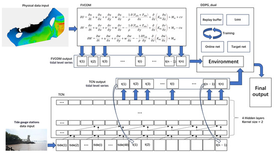
Figure 1.
The architecture of DNR model.
3.1. FVCOM Hydrodynamic Model
FVCOM is a three-dimensional, unstructured-grid, prognostic modeling system designed for free-surface flow simulations [36]. Its computational efficiency and geometric flexibility enable precise representation of complex coastal and marine environments, including irregular bathymetries, islands, and engineered structures. The model’s governing equations incorporate fundamental hydrodynamic principles, solving coupled systems for momentum, mass continuity, temperature, salinity, and density fields. The core formulation is governed by the following equation [37]:
where x, y, z, u, v, and w represent the three coordinate axes in the Cartesian coordinate system and their corresponding velocity components, respectively. denotes density; represents hydrostatic pressure; denotes non-hydrostatic pressure; c is the Coriolis parameter. is the vertical eddy diffusion coefficient. , , and are the momentum components in the three directions. This dynamic process is constructed on an unstructured grid to simulate wave propagation. To achieve this, a refined grid was established for the simulated water area, as shown in Figure 2 [38].
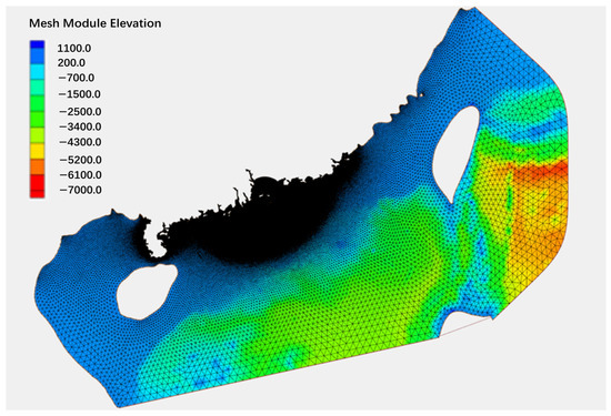
Figure 2.
The grid of simulation region.
3.2. Temporal Convolutional Network
Temporal Convolutional Network (TCN) is a deep learning model specifically designed for processing sequential data [39], combining the parallel computing advantages of Convolutional Neural Networks (CNNs) with the long-term dependency modeling capabilities of Recurrent Neural Networks (RNNs). The structure of TCN is shown in Figure 3.
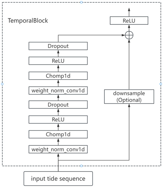
Figure 3.
The architecture of TCN.
The entire TCN is composed of 4 stacked structures described above, with the output of each TemporalBlock layer serving as the input to the next TemporalBlock layer. The core TemporalBlock implementation in TCN is as follows: TCN employs causal convolution to ensure the model only relies on current and past time step data when predicting the current time step, without using future information. By applying padding operations to the convolution kernel, it guarantees that the t-th time step in the output tidal level prediction sequence only convolves with the t-th and prior time steps in the input tidal level sequence. This preserves the causality of time series prediction and prevents future information from leaking into the current prediction moment. This process can be expressed as follows:
where performs weight normalization to avoid vanishing and exploding gradients, enhancing model generalization. implements causal convolution, and represents the corresponding hidden layer representation. To maintain consistent input–output lengths, TCN uses Chomp1d to trim redundant padded portions from convolution results. To capture long-range dependencies, TCN employs dilated convolution [39], which inserts dilation between kernel elements to exponentially expand the receptive field without increasing parameter count, enabling the model to capture long-distance dependencies. The formula for dilated convolutions is expressed as follows [39]:
where represents the convolutional weights, and d is the dilation rate, which determines how many steps between inputs are used in the convolution. When , the convolution involves consecutive inputs. refers to the output of the hidden layer, and represents the input sequence from the previous layer, where the input is gathered according to the dilation rate d. Finally, a residual connection is used to directly add the input to the output of the convolutional layer. This helps alleviate the vanishing gradient problem, accelerates training, and, through the activation function, produces the output of the TemporalBlock. This process is expressed as follows:
where is the output predicting the tidal level at time , and are the tidal input sequence of length k, consisting of the tidal levels at time t and earlier. is a downsample layer, which is essentially a 1D convolutional layer that is used only when the input and output dimensions of the hidden layer are not equal. The purpose is to ensure dimensionality matching when performing residual connections. stands for Temporal Block, which can be specifically described by the following equation:
where are the tidal input sequence of length k.
It is important to note that, in this study, actually predicts the tidal level at time . Tidal level prediction can be viewed as an autoregressive prediction, where the target tidal level prediction output is defined as the result of shifting the input tidal levels one time step forward [39].
3.3. DDPG_Dual Moudle
Deep Deterministic Policy Gradient (DDPG) is a deep reinforcement learning method that provides an intelligent solution for combining predictions from base models. Specifically, DDPG is an algorithm used for reinforcement learning in continuous action spaces [40]. It combines deep neural networks with deterministic policy gradient methods, effectively addressing decision-making problems in high-dimensional states and continuous action spaces. The core idea is to enable efficient learning of agents in complex environments through the collaborative optimization of the policy network and value network. The structure of the DDPG algorithm consists of four key components: the current policy network (Actor), the target policy network (Target Actor), the current value network (Critic), and the target value network (Target Critic). The Actor network outputs deterministic actions based on the current state, while the Critic network evaluates the value of these actions. The target networks provide stable training objectives through soft updates, reducing oscillations during the policy update process. The experience replay mechanism improves training efficiency by randomly sampling from historical experiences, breaking data correlations.
The DDPG_dual structure used in this study is shown in Figure 4. The online network and the target network are constructed separately, with both networks having identical structures. The online network is used for real-time decision making, while the target network is used for training and learning. The Actor network and Critic network are deployed on both the online and target networks. The Actor network is responsible for calculating actions based on the environmental state. The design of the Critic network is intended to assist in evaluating actions, as the environment cannot always provide concise feedback for each action step. In DDPG_dual, the action is formed through a dual-channel network and an attention gate control network. The dual-channel network consists of the mainstream network and the extreme flow network. Note that, the dashed red region are the two parallel branches which are a main stream and an extreme stream. The mainstream network handles regular tidal level changes, while the extreme flow network specializes in processing extreme regions such as wave peaks and troughs. The outputs of these two networks are dynamically fused through the attention gate control network. The Actor network receives the current environmental state and outputs the final tidal level prediction, . The score output from the Critic network, , comprehensively considers the influences of the current state and action . This is also formed through the dual-channel network and the attention gate control network. The action is fed back into the environment to obtain the reward information and transition to the next state . The data generated through this process are stored in the experience replay buffer for parameter updates across the entire DDPG_dual.
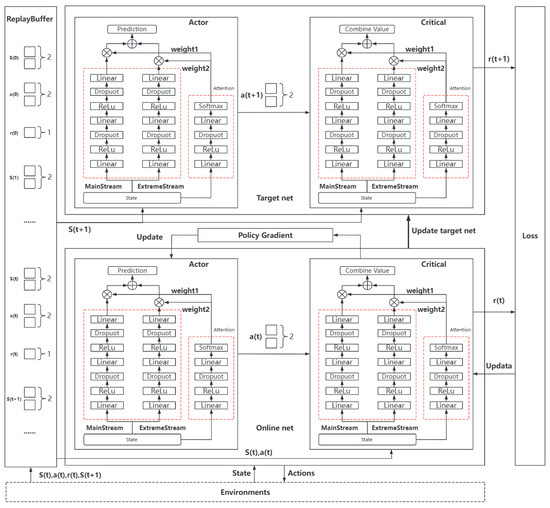
Figure 4.
The structure of DDPG_dual.
The loss function of the Critic network in DDPG_dual consists of the general mean squared error and the extreme point mean squared error, which are defined as follows:
where represents the current Critic network’s Q-value estimate for the current state–action pair, which is the calculated immediate reward and the estimated future reward. is the target Critic network’s Q-value estimate for the next state–action pair. is the loss for extreme points, designed to enable the network to better combine the base model’s predictions for tidal extreme points. is defined as follows:
where is the extreme point mask, which is set to 1 when an extreme point is predicted, and 0 otherwise. The loss function for the Actor network corresponding to is then defined as follows:
where s represents all states obtained from the experience replay buffer, and denotes the action taken for the corresponding state is the mean function. The calculation of is performed using the following formula:
where is the current reward, indicates whether it is a terminal state, is the discount factor, and the final term represents the target network’s Q-value estimate for the next state and action.
The overall workflow of DDPG_dual is as follows: it receives tidal level prediction value sequences from two base models, FVCOM, and TCN and uses them as input for the environmental state. DDPG_dual then focuses on learning how to effectively combine these predictions and ultimately outputs the optimized tidal level prediction results.
4. Experiments
The super typhoon “Mangkhut” in 2018 was a notable storm of the Pacific typhoon season, recognized for its intense strength, broad impact, and devastating power, resulting in severe disasters across multiple regions [41]. This experiment used this case as the experimental object. Observation data from six tidal stations in the South China Sea were selected for study. The specific study area is shown in Figure 5.
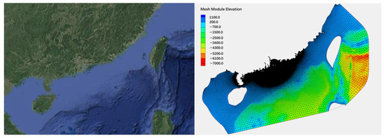
Figure 5.
The study area of this work is in the South China Sea, and the grid of the numerical model covers the main research scope. Map data © GoogleMap contributors (https://www.google.com/maps (accessed on 20th July 2025)).
Data Sources. This study selected a total of six tidal stations in the South China Sea region. The names of each station and their corresponding longitude and latitude coordinates are shown in Table 1.

Table 1.
Stations’ longitude and latitude coordinates.
The data used in this study come from the water level observation records of six tidal stations in the South China Sea, covering the period from January to September 2018 (a total of 9 months). The data from each tidal station for the period from January to August 2018 were used for training the neural network, while the data from September were reserved for validation. All tidal stations recorded water levels every hour, resulting in 24 recordings per day. During the data processing phase, we pre-processed the data from the six tidal stations, disgrading some missing values, and then fed the processed data into the neural network for training. After training the neural network, we used it to predict the water levels for 312 h starting from 00:00 on 3 September 2018. At the same time, the FVCOM model performed the same prediction task, generating corresponding prediction results for the six tidal stations. Among the six sets of prediction results obtained, we selected the prediction data from five tidal stations and divided them into a training set and a test set in an approximately 80:20 ratio for use in the reinforcement learning fusion module. The remaining 312 h of prediction data from one tidal station were used entirely to validate the generalization ability of the DNR model.
Evaluation Metrics. To evaluate the performance of our proposed model, we adopted the Mean Absolute Error (MAE), Root Mean Square Error (RMSE), Pearson correlation coefficient, and Nash–Sutcliffe Efficiency (NSE), which are commonly used metrics for tidal level prediction tasks. Additionally, we conducted a detailed comparison with other models.
4.1. Experimental Setup
This study was equipped with 32 GB of RAM and an NVIDIA RTX 4070Ti GPU with 12 GB of VRAM for hardware, as well as an Intel 14th-generation processor for the CPU. On the software side, VSCode was used as the development environment. For more detailed setup information, please refer to Table 2.
Table 2.
Experimental operating environment.
The key settings of the FVCOM model’s nml configuration file are shown in Table 3. Considering that the FVCOM simulation has an initial cold start period, the simulation was run in advance for a period of time, and the first 48 h of the prediction results were discarded. That is, the actual prediction started from 00:00 on 3 September 2018, with prediction results output every hour. In Table 3, START_DATE represents the start time of the FVCOM prediction, and END_DATE denotes the end time of the prediction. STARTUP_TYPE is used to specify the startup mode of the model. NC_FIRST_OUT refers to the start time for outputting prediction results in the NetCDF file, while NC_OUT_INTERVAL defines the time interval for outputting prediction values in the NetCDF file. As for WIND_ON, it indicates whether the wind field file is enabled, with “F” meaning that the wind field file is not enabled.
Table 3.
FVCOM configuration.
As shown in Table 3, the model employed a time step of 3 s. The grid design incorporated a minimum resolution of approximately 500 m, with simulated current velocities not exceeding 4 m/s in the model outputs. The CFL condition analysis confirms that values remained substantially below 1. Furthermore, the wet/dry treatment threshold was set to 0.05 m following FVCOM manual recommendations, significantly enhancing the model’s stability in nearshore simulations. Referencing the grid resolution settings from existing FVCOM studies [42], our grid generation followed these principles: coastal zones, estuaries, and bays characterized by high gradients were refined to 500 m, while open sea areas gradually transitioned to 30 km. The geometric fidelity of shorelines and isobaths was maintained using high-resolution topographic and shoreline mapping data provided by RESDC.
The general hyperparameter settings for the TCN deep learning model are shown in Table 4. The hyperparameters were configured based on the TCN paper and experimental observations from this study. The number of training epochs was set to 400, because the loss curve indicated convergence after approximately 300 epochs, and models trained with 400 epochs exhibited comparable performance to those trained with 500 epochs.
Table 4.
TCN hyperparameter setting.
The common hyperparameters for the other deep learning models used for comparison can be set according to the settings in the table above. For all deep learning models, we selected water level data from January to August 2018 as the training set. The model input was uniformly set as the 48 h of observed data prior to the prediction, while the output focused on predicting the water level for the next hour. Based on this setup, approximately 5500 data points were generated for each station to train the model. After training the model, we used a rolling prediction approach for water level forecasting. Specifically, the first 48 h of data before 00:00 on 1st September were used to predict the water level for the next hour. Then, this prediction result was combined with the previous 47 h of actual data to form a new input for predicting the water level for the second hour. This process continued until 48 h of water level predictions were completed. Next, the 48 h observed water level data from 1st to 2nd September were used to predict the water levels from 3rd to 4th September, and so on, until predictions were made through 23:00 on 15th September, totaling 360 h of predictions. After comparing the prediction performance of the four deep learning models and the ARIMA model, we selected the best-performing model. We then used approximately 80% of the predicted data from five tidal stations for training the fusion model. Finally, we tested the fusion model using the remaining 48 h of prediction data from these five stations, as well as the full prediction data from another station that was not involved in fusion model training.
The hyperparameter settings for the fusion model, DDPG_dual, are shown in Table 5. The state dimension is 24, which means the input to the fusion network consists of 24 data points, combining 12-h predicted water levels from both FVCOM and TCN. The fusion network is responsible for outputting two weights, which are used to perform a weighted fusion of the final set of predictions from the FVCOM and TCN models, resulting in the final prediction from the fusion model.
Table 5.
DDPG_dual hyperparameter setting.
4.2. Experimental Result
This section provides a detailed analysis of the experimental results, focusing primarily on the four metrics mentioned earlier. Comparative analysis of similar models was conducted in both the deep learning prediction model phase and the fusion model phase, with the aim of comprehensively evaluating the performance and effectiveness of the proposed fusion model.
Firstly, we used the FVCOM model to predict the tidal levels at six tidal stations. Since FVCOM starts simulations in cold-start mode, to ensure the accuracy of the prediction results, we discarded the first 48 h of data after the simulation began and selected the subsequent 312 h of data as the FVCOM prediction results. Among these, for the five stations used for fusion model training, we specifically selected the last 48 h of data, which were not involved in the fusion model training, for display (the previous 250 h of prediction data were used for fusion model training). For station BHI, which was not involved in fusion model training, we displayed its complete 312-h prediction results. In Figure 6, the predicted results for each station are shown by green lines, while the corresponding actual tidal level data is presented by red lines.

Figure 6.
Comparison between 48-h tidal level predictions from the FVCOM numerical model and observational data: (a) BHI. (b) DFG (c) DWS. (d) QLN. (e) SWI. (f) WZU.
(1) Quantitative Comparative Analysis of Models: This section focuses on the performance comparison between two categories of models: first, the comparison between deep learning models and the ARIMA model, and second, the performance comparison among different fusion models.
First, we compared the performance between the deep learning models and the ARIMA model. The deep learning models included TCN (Temporal Convolutional Network), RNN (Recurrent Neural Network), LSTM (Long Short-Term Memory Network), and VIT (Vision Transformer). We used these models to predict the tidal levels at six tidal stations, with the performance metrics of the models for each station shown in Table 6. For each station, the numbers marked in red represent the minimum value for the corresponding model on that metric (note that for MAE, which is Mean Absolute Error, and RMSE, which is Root Mean Square Error, smaller values are better). The numbers marked in blue represent the maximum value for the corresponding model on that metric (where Pearson correlation coefficient and NSE, the Nash–Sutcliffe Efficiency, are better when larger).
Table 6.
Performance comparison between deep learning models and the ARIMA model.
Overall, the TCN model demonstrated the best performance in this study, achieving the smallest Mean Absolute Error (MAE) at most stations while also attaining the highest correlation coefficient and Nash–Sutcliffe Efficiency (NSE). This outstanding performance is primarily attributed to the unique architecture of the TCN: by stacking convolutional layers with different dilation rates, the TCN can effectively capture patterns at various scales and long-term dependencies within sequential data. This structural feature makes the TCN particularly effective in modeling long-term temporal correlations. Additionally, the convolutional operations used in TCN are shift-invariant, meaning that regardless of the time position of the input sequence, the learned features remain valid. This characteristic further enhances the robustness of the TCN model, enabling it to better adapt to temporal shifts and dynamic changes in sequential data, thereby significantly improving prediction accuracy. The LSTM model followed closely, exhibiting second-best performance, while the traditional RNN model ranked behind the LSTM. This outcome is expected, as LSTM, an improved version of RNN, has a distinct advantage in handling long-term dependencies in sequential data. In contrast, the VIT model performed poorly in this tidal level forecasting task. Originally designed for image recognition, the VIT model’s core idea is to divide an image into multiple patches and arrange them into a sequence, similar to the processing of natural language. While some adjustments can be made to the network, the VIT model still struggled to achieve satisfactory prediction results for sequential data like tidal level forecasting. The ARIMA model performed the worst in this study. Across all data metrics, the TCN model, with its excellent performance and robustness, emerged as the preferred choice for the deep learning prediction module.
After obtaining the prediction data from FVCOM and the deep learning model TCN, we conducted a series of tests and comparisons on five reinforcement learning fusion models: DDPG_dual, DDPG, PPO, DQN, and DDQN. Specifically, we selected approximately 80% of the prediction data from five stations for training the fusion models and used the last 48 h of prediction data for fusion testing. Additionally, for the station that did not participate in the fusion model training (BHI), we used 312 h of prediction data for fusion testing. The results are presented in Table 7. For comparison purposes, the performance metrics of the FVCOM and TCN models are also listed in the table. As in Table 6, the numbers marked in red indicate the minimum value achieved by the corresponding model on that metric, while the numbers marked in blue indicate the maximum value achieved.
Table 7.
Comparison of fusion models, FVCOM, and TCN.
Overall, the DDPG_dual model demonstrated the best predictive performance across all tide stations, outperforming both the TCN model and the DDPG model. This can primarily be attributed to the addition of a specialized module for handling extremes in the actor and critic networks of the DDPG_dual model compared with the DDPG model. This module is more effective in predicting wave peaks and troughs, leading to predictions that are closer to the real data. This will be further validated in the subsequent ablation experiments.
The DDPG model showed strong performance at the five training stations, second only to the DDPG_dual model. However, at the BHI station, its Mean Absolute Error (MAE) and Root Mean Square Error (RMSE) still lagged behind the TCN model. Notably, the DDPG_dual model also achieved the best results when conducting fusion predictions at the unseen BHI station. This suggests that the generalization ability of the DDPG_dual model is stronger compared with the DDPG model. It is worth emphasizing that, within the spatiotemporal scope influenced by Typhoon Mangkhut, the proposed ensemble learning DNR model effectively integrated the prediction sequences from two base models and achieved accurate tidal level forecasting. This also further validates robustness of the proposed method under extreme weather conditions.
A comparison with previously mentioned related studies reveals that our proposed DNR model achieved a correlation coefficient above 0.9 even over a 48-h prediction horizon, outperforming the correlation coefficient reported in that study [27] for 24-h tidal predictions. Compared with the results of this study [14], the correlation coefficient of our model’s 48-h tidal prediction (with an average of 0.9403 across six stations) remains close to that of the 50-h tidal prediction curve (average 0.9511) reported in their study under the influence of Typhoon Mangkhut. Overall, the performance of our proposed model can be considered satisfactory.
(2) Qualitative Comparison: We also plotted the prediction curves of each model. Figure 7 shows the prediction curves of the deep learning models compared against the ARIMA model, while Figure 8 presents the prediction curves of the various fusion models. In Figure 8, for each subplot, the red solid line represents the real tide level curve, and the black solid line represents the prediction curve of the DDPG_dual model. From the figure, it is clear that the DDPG_dual model generally fits the real curve quite well. In most cases, compared to the DDPG model, it is able to more accurately capture the peaks and troughs of the real curve, demonstrating superior predictive performance. However, there are certain time points where the DDPG_dual model’s predictions still show some shortcomings. For example, around the 10th hour at the SWI station and around the 13th h at the DWS station, there are significant discrepancies between the predicted and actual tide levels. The DQN and DDQN models, due to their discrete action selection, have certain limitations in their fusion performance compared to the DDPG model. The PPO fusion model, being the most complex of the models tested, not only requires longer training times but also has a slower convergence rate. Although some patterns in the tide level changes can be observed in its predictions, the prediction errors are large, making it difficult to meet the precision requirements for practical applications.
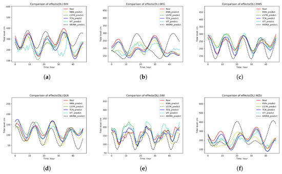
Figure 7.
Prediction curves of deep learning models and ARIMA model: (a) BHI. (b) DFG (c) DWS. (d) QLN. (e) SWI. (f) WZU.
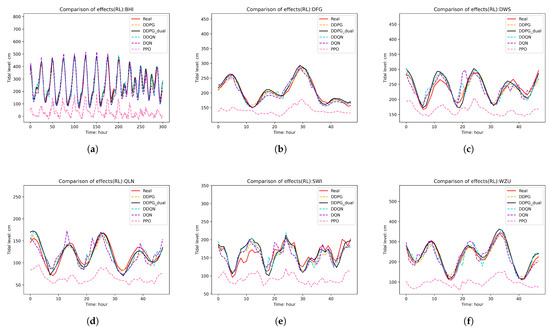
Figure 8.
Prediction curves of fusion models: (a) BHI. (b) DFG (c) DWS. (d) QLN. (e) SWI. (f) WZU.
(3) Ablation Study: To further enhance the performance of the fusion model, we made two key improvements to the original DDPG model. On one hand, we introduced a dual-channel mechanism to strengthen the model’s ability to process input information, thereby improving the fusion effect. On the other hand, we optimized the original reward mechanism to encourage the model to focus more on accurately handling extreme values during training.
Specifically, we named the original DDPG model as DDPG_O_1. After introducing the dual-channel mechanism, the model was named DDPG_dual. Further adjustments to the reward mechanism based on DDPG_dual resulted in a model named DDPG_d_e. To validate the effectiveness of the newly added structures, we tested the above models using the same dataset. The average absolute errors (MAE) for each model are shown in Table 8. Here, DDPG_d_e (128) and DDPG_d_e (256) represent models with hidden layer neuron counts of 128 and 256, respectively. The error units are unified in centimeters (cm).
Table 8.
Model prediction error.
As seen in Table 8, the basic fusion model DDPG had an average error of 12.285 cm. After incorporating the dual-channel attention mechanism, the average error dropped to 11.624 cm. Further improving the reward mechanism reduced the average error to 11.228 cm. When the hidden layer was adjusted to 256 neurons, the average error decreased even further to 10.248 cm. Overall, these adjustments effectively enhanced the fusion performance of the DDPG model, resulting in approximately a 16% reduction in prediction error. During the optimization of DDPG_dual, we implemented the aforementioned improvements and plotted their prediction curves (Figure 9). The results demonstrate that the optimal model outperformed others in closely matching the extreme values of the ground truth curve. For instance, at tidal station DWS, it showed significantly better alignment with actual measurements at the first trough, third trough, and second peak. Similar improvements were observed at station SWI. Moreover, the best performing model maintained superior consistency with real observations across all remaining tidal stations.
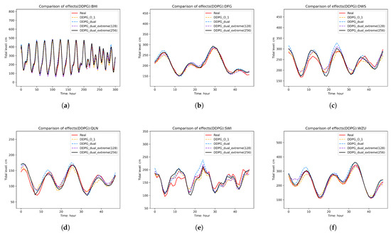
Figure 9.
Performance comparison of different DDPG model improvement strategies: (a) BHI. (b) DFG (c) DWS. (d) QLN. (e) SWI. (f) WZU.
5. Conclusions
This paper focuses on the problem of ocean tide level prediction under storm surge conditions, with the core objective of accurately predicting the ocean tide level with minimal error. Given the limitations of a single model in terms of predictive capability, this paper innovatively proposes an ensemble learning-based DNR model. The model leverages the improved reinforcement learning model DDPG_dual to combine the predictions of base models, successfully integrating the advantages of deep learning models and the FVCOM model. Compared to base models, the DNR model achieved significant improvements in prediction accuracy. Through validation with real-world cases, Typhoon Mangkhut, the DNR model demonstrated exceptional predictive capabilities. In particular, under storm surge conditions and when facing unseen environments (such as the BHI station), the DNR model outperformed single models, fully proving its adaptability and reliability in complex environments.Moreover, through ablation studies, this paper further confirms that the two key improvements made to DDPG significantly reduce the tide prediction errors, providing strong theoretical support for model optimization.
We attribute the effectiveness of the DNR model primarily to the following factors: The FVCOM numerical model, based on hydrodynamic equations, captures the physical principles of tidal wave propagation but remains sensitive to boundary conditions; the TCN neural network excels at extracting nonlinear temporal features from historical data but lacks physical constraints. The integration of both preserves physical consistency while enhancing the capability to model complex patterns. The DDPG_dual framework leverages an actor–critic network to dynamically evaluate the predictive reliability of each base model across spatiotemporal conditions, generating adaptive fusion weights that outperform traditional static weighting methods. Furthermore, the policy gradient update mechanism in reinforcement learning learns fusion rules through environmental interactions rather than direct fitting of training data, reducing dependence on annotated datasets and mitigating overfitting in small-sample scenarios.
The DNR model requires extended data duration, which implies that longer monitoring periods are needed to accumulate sufficient observations for optimal model calibration and stable convergence; in particular, capturing seasonal cycles and infrequent extremes typically demands sustained records rather than short-term datasets. In addition, FVCOM computations are time consuming. Running the model, especially at the spatial and temporal resolutions employed in this paper, entails substantial runtime. Future research could explore further ways to integrate the DNR model with other advanced prediction techniques or data sources to address even more complex and dynamic marine environments. This includes the impact of extreme weather events, changes in marine ecosystems, and other factors on tide prediction. Additionally, further investigations can be made to optimize the model’s parameter settings and training strategies, improving the model’s computational efficiency and generalization ability. This will ensure that the model can more quickly and accurately provide tide prediction information in real-world applications, offering stronger support for ocean disaster warnings and emergency responses.
Author Contributions
Conceptualization, X.C. and Y.W.; methodology, G.Z. and Y.W.; software, X.C. and G.Z.; validation, X.C., G.Z., and Y.W.; formal analysis, G.Z.; investigation, X.C.; resources, Y.W.; data curation, Y.W.; writing—original draft preparation, X.C. and G.Z.; writing—review and editing, Y.W.; visualization, G.Z.; supervision, X.C.; project administration, X.C.; funding acquisition, X.C. and Y.W. All authors have read and agreed to the published version of the manuscript.
Funding
The work was supported by the “CUG Scholar” Scientific Research Funds at the China University of Geosciences (Wuhan) (Project No. 2023080).
Institutional Review Board Statement
Not applicable.
Informed Consent Statement
Not applicable.
Data Availability Statement
The raw data supporting the conclusions of this article will be made available by the authors on request. The code for data analysis is available upon request from the authors.
Conflicts of Interest
The authors declare no conflicts of interest.
References
- Wadey, M.P.; Haigh, I.D.; Nicholls, R.J.; Brown, J.M.; Horsburgh, K.; Carroll, B.; Gallop, S.L.; Mason, T.; Bradshaw, E. A Comparison of the 31 January–1 February 1953 and 5–6 December 2013 Coastal Flood Events Around the UK. Front. Mar. Sci. 2015, 2, 84. [Google Scholar] [CrossRef]
- Bernier, N.B.; Hemer, M.; Mori, N.; Appendini, C.M.; Breivik, O.; de Camargo, R.; Casas-Prat, M.; Duong, T.M.; Haigh, I.D.; Howard, T.; et al. Storm surges and extreme sea levels: Review, establishment of model intercomparison and coordination of surge climate projection efforts (SurgeMIP). Weather Clim. Extrem. 2024, 45, 100689. [Google Scholar] [CrossRef]
- Mori, N.; Kato, M.; Kim, S.; Mase, H.; Shibutani, Y.; Takemi, T.; Tsuboki, K.; Yasuda, T. Local amplification of storm surge by Super Typhoon Haiyan in Leyte Gulf. Geophys. Res. Lett. 2014, 41, 5106–5113. [Google Scholar] [CrossRef] [PubMed]
- Xuan, J.; Ding, R.; Zhou, F. Storm surge risk under various strengths and translation speeds of landfalling tropical cyclones. Environ. Res. Lett. 2021, 16, 124055. [Google Scholar] [CrossRef]
- Ali Ghorbani, M.; Khatibi, R.; Aytek, A.; Makarynskyy, O.; Shiri, J. Sea water level forecasting using genetic programming and comparing the performance with Artificial Neural Networks. Comput. Geosci. 2010, 36, 620–627. [Google Scholar] [CrossRef]
- Dean, R.G.; Dalrymple, R.A. Coastal Processes with Engineering Applications; Cambridge University Press: Cambridge, UK, 2004. [Google Scholar]
- Li, X.; Zhou, S.; Wang, F. A CNN-BiGRU sea level height prediction model combined with bayesian optimization algorithm. Ocean Eng. 2025, 315, 119849. [Google Scholar] [CrossRef]
- Hashemi, M.R.; Spaulding, M.L.; Shaw, A.; Farhadi, H.; Lewis, M. An efficient artificial intelligence model for prediction of tropical storm surge. Nat. Hazards 2016, 82, 471–491. [Google Scholar] [CrossRef]
- Jian, L.; Wang, X.; Jiang, W.; Hao, H.; Xi, R.; Yang, L. Improved tide level prediction model combined GA-BP neural networks and GNSS SNR data. Adv. Space Res. 2024, 74, 1595–1608. [Google Scholar] [CrossRef]
- Kuo, J.T. Everywhere in the ocean waters. In Tidal Hydrodynamics; John Wiley: New York, NY, USA, 1991; p. 61. [Google Scholar]
- Reichstein, M.; Camps-Valls, G.; Stevens, B.; Jung, M.; Denzler, J.; Carvalhais, N.; Prabhat, M. Deep Learning and Process Understanding for Data-Driven Earth System Science. Nature 2019, 566, 195–204. [Google Scholar] [CrossRef]
- Balas, C.E.; Koç, M.L.; Tür, R. Artificial neural networks based on principal component analysis, fuzzy systems and fuzzy neural networks for preliminary design of rubble mound breakwaters. Appl. Ocean Res. 2010, 32, 425–433. [Google Scholar] [CrossRef]
- Yin, J.; Wang, N.; Hu, J. A hybrid real-time tidal prediction mechanism based on harmonic method and variable structure neural network. Eng. Appl. Artif. Intell. 2015, 41, 223–231. [Google Scholar] [CrossRef]
- El-Diasty, M.; Al-Harbi, S. Development of wavelet network model for accurate water levels prediction with meteorological effects. Appl. Ocean Res. 2015, 53, 228–235. [Google Scholar] [CrossRef]
- Primo de Siqueira, B.V.; de Moraes Paiva, A. Using neural network to improve sea level prediction along the southeastern Brazilian coast. Ocean Model. 2021, 168, 101898. [Google Scholar] [CrossRef]
- Bento, P.; Pombo, J.; Mendes, R.; Calado, M.; Mariano, S. Ocean wave energy forecasting using optimised deep learning neural networks. Ocean Eng. 2021, 219, 108372. [Google Scholar] [CrossRef]
- Cheng, R.T.; Gartner, J.W. Harmonic analysis of tides and tidal currents in South San Francisco Bay, California. Estuar. Coast. Shelf Sci. 1985, 21, 57–74. [Google Scholar] [CrossRef]
- Salmun, H.; Molod, A. The use of a statistical model of storm surge as a bias correction for dynamical surge models and its applicability along the US East Coast. J. Mar. Sci. Eng. 2015, 3, 73–86. [Google Scholar] [CrossRef]
- Lin, M.; Juang, W.; Tsay, T. Applications of the mild-slope equation to tidal computations in the Taiwan Strait. J. Oceanogr. 2000, 56, 625–642. [Google Scholar] [CrossRef]
- Doodson, A.T. The harmonic development of the tide-generating potential. Proc. R. Soc. Lond. Ser. A Contain. Pap. A Math. Phys. Character 1921, 100, 305–329. [Google Scholar]
- Foreman, M.; Henry, R. The harmonic analysis of tidal model time series. Adv. Water Resour. 1989, 12, 109–120. [Google Scholar] [CrossRef]
- Box, G.E.; Jenkins, G.M.; Reinsel, G.C.; Ljung, G.M. Time Series Analysis: Forecasting and Control; John Wiley & Sons: Hoboken, NJ, USA, 2015. [Google Scholar]
- Mahjoobi, J.; Mosabbeb, E.A. Prediction of significant wave height using regressive support vector machines. Ocean Eng. 2009, 36, 339–347. [Google Scholar] [CrossRef]
- Tsai, C.; Lee, T. Back-propagation neural network in tidal-level forecasting. J. Waterw. Port Coast. Ocean Eng. 1999, 125, 195–202. [Google Scholar] [CrossRef]
- Juan, N.P.; Valdecantos, V.N. Review of the application of Artificial Neural Networks in ocean engineering. Ocean Eng. 2022, 259, 111947. [Google Scholar] [CrossRef]
- Lee, T. Back-propagation neural network for long-term tidal predictions. Ocean Eng. 2004, 31, 225–238. [Google Scholar] [CrossRef]
- Bertin, X.; Fortunato, A.B.; Oliveira, A. A modeling-based analysis of processes driving wave-dominated inlets. Cont. Shelf Res. 2009, 29, 819–834. [Google Scholar] [CrossRef]
- Wenzel, M.; Schröter, J. Reconstruction of regional mean sea level anomalies from tide gauges using neural networks. J. Geophys. Res. Ocean. 2010, 115, C08013. [Google Scholar] [CrossRef]
- Filippo, A.; Torres, A.R., Jr.; Kjerfve, B.; Monat, A. Application of Artificial Neural Network (ANN) to improve forecasting of sea level. Ocean Coast. Manag. 2012, 55, 101–110. [Google Scholar] [CrossRef]
- Bai, L.; Xu, H. Accurate estimation of tidal level using bidirectional long short-term memory recurrent neural network. Ocean Eng. 2021, 235, 108765. [Google Scholar] [CrossRef]
- El-Diasty, M.; Al-Harbi, S.; Pagiatakis, S. Hybrid harmonic analysis and wavelet network model for sea water level prediction. Appl. Ocean Res. 2018, 70, 14–21. [Google Scholar] [CrossRef]
- Lin, C.; Xu, J.; Jiang, D.; Hou, J.; Liang, Y.; Zou, Z.; Mei, X. Multi-model ensemble learning for battery state-of-health estimation: Recent advances and perspectives. J. Energy Chem. 2025, 100, 739–759. [Google Scholar] [CrossRef]
- Song, Y.; Suganthan, P.N.; Pedrycz, W.; Ou, J.; He, Y.; Chen, Y.; Wu, Y. Ensemble reinforcement learning: A survey. Appl. Soft Comput. 2023, 149, 110975. [Google Scholar] [CrossRef]
- Breiman, L. Bagging predictors. Mach. Learn. 1996, 24, 123–140. [Google Scholar] [CrossRef]
- Schapire, R.E. The Boosting Approach to Machine Learning: An Overview. In Nonlinear Estimation and Classification; Denison, D.D., Hansen, M.H., Holmes, C.C., Mallick, B., Yu, B., Eds.; Springer: New York, NY, USA, 2003; pp. 149–171. [Google Scholar]
- Wang, N.; Ge, J. Predictions of saltwater intrusion in the Changjiang Estuary: Integrating Machine learning methods with FVCOM. J. Hydrol. 2025, 653, 132739. [Google Scholar] [CrossRef]
- Chen, C.; Beardsley, R.C.; Cowles, G.; Qi, J.; Lai, Z.; Gao, G.; Stuebe, D.; Liu, H.; Xu, Q.; Xue, P.; et al. FVCOM User Manual v3.1.6; SMAST/UMASSD: Dartmouth, MA, USA, 2013; SMAST/UMASSD-13-0701. [Google Scholar]
- Wang, Y.; Chen, X.; Wang, L. Differential Semi-Quantitative Urban Risk Assessment of Storm Surge Inundation. ISPRS Ann. Photogramm. Remote Sens. Spat. Inf. Sci. 2022, 10, 177–185. [Google Scholar] [CrossRef]
- Bai, S.; Kolter, J.Z.; Koltun, V. An Empirical Evaluation of Generic Convolutional and Recurrent Networks for Sequence Modeling. arXiv 2018, arXiv:1803.01271. [Google Scholar] [CrossRef]
- Lillicrap, T.P.; Hunt, J.J.; Pritzel, A.; Heess, N.; Erez, T.; Tassa, Y.; Silver, D.; Wierstra, D. Continuous control with deep reinforcement learning. arXiv 2019, arXiv:1509.02971. [Google Scholar]
- Li, Y.; Wu, J.; Tang, R.; Wu, K.; Nie, J.; Shi, P.; Li, N.; Liu, L. Vulnerability to typhoons: A comparison of consequence and driving factors between Typhoon Hato (2017) and Typhoon Mangkhut (2018). Sci. Total Environ. 2022, 838, 156476. [Google Scholar] [CrossRef]
- Premathilake, L.; Khangaonkar, T. FVCOM-Plume–A Three-Dimensional Lagrangian Outfall Plume Dilution and Transport Model for Dynamic Tidal Environments: Model Development. Mar. Pollut. Bull. 2019, 149, 110554. [Google Scholar] [CrossRef]


Disclaimer/Publisher’s Note: The statements, opinions and data contained in all publications are solely those of the individual author(s) and contributor(s) and not of MDPI and/or the editor(s). MDPI and/or the editor(s) disclaim responsibility for any injury to people or property resulting from any ideas, methods, instructions or products referred to in the content. |
© 2025 by the authors. Licensee MDPI, Basel, Switzerland. This article is an open access article distributed under the terms and conditions of the Creative Commons Attribution (CC BY) license (https://creativecommons.org/licenses/by/4.0/).