Data-Driven Modeling of Floating Offshore Wind Turbine Dynamics: An Optimized Artificial Neural Network Approach Using OC5 Experimental Data

Abstract

The global transition of offshore wind energy into deep-water environments necessitates precise modeling of the complex, nonlinear dynamic responses of floating offshore wind turbines (FOWTs) to stochastic loads. Traditional industry-standard simulation tools often rely on potential flow theory, which neglects critical viscous effects and requires manual, empirical tuning of damping coefficients, reducing model reliability, while CFD modeling demands large computational resources. This paper introduces an application of advanced neural network techniques to model the coupled dynamic response of FOWTs under varied ocean conditions, reducing the simulation time required for training high-fidelity models. The architecture was trained using experimental data from the OC5 semi-submersible platform under the LC4.1 load case and further validated across a matrix of heterogeneous conditions, encompassing steady, turbulent, and irregular wind and wave environments. Results demonstrate exceptional predictive accuracy across coupled degrees of freedom (Heave, Pitch, and Surge), with the model achieving a coefficient of determination (${\mathrm{R}}^2>0.9$) and maintaining superior phase coherence without discernible time lag. Power spectral density analysis confirms the model’s robust ability to capture resonant frequencies and hydrodynamic restoration across varied sea states. This data-driven framework provides a robust, near-instantaneous alternative for simulating FOWTs global dynamics. By successfully capturing complex nonlinear interactions and inertial effects, the methodology enables rapid decision-making in preliminary design, real-time digital twinning, and accelerated long-term fatigue analysis for safety-critical offshore applications.

1. Introduction

The global offshore wind energy sector is undergoing transformative growth, essential for accessing deep-water resources where most wind potential resides. With the global installed capacity reaching 68,258 MW by the end of 2023 and the floating offshore wind pipeline totaling 104,399 MW, floating offshore wind turbine technology is rapidly maturing [1]. This shift subjects FOWTs to more severe environmental loads, causing strong structural vibrations and significant fatigue damage to the structure and mooring systems. Consequently, accurately predicting the 6-degree-of-freedom (6DOF) motion and long-term extreme responses is crucial for safety and certification, a task traditionally reliant on computationally intensive methods like Full Long-term Analysis (FLTA) [2,3,4]. To achieve the required speed and accuracy for lifetime analysis, advanced data-driven approaches, particularly those utilizing neural networks (NNs), have become an indispensable alternative for modeling these complex coupled dynamics [5].

Artificial neural networks have long provided a versatile computational framework for modeling, classification, and prediction, leveraging their capacity to map complex, nonlinear input–output relationships that resist analytical solution. In mechanical engineering, ANNs are utilized for design and optimization problems due to their efficiency in managing high-dimensional data [6]. This cross-disciplinary success in handling complex nonlinear dynamics establishes the foundational suitability of ANNs for FOWT modeling, where coupled aerodynamic, hydrodynamic, and mooring forces interact nonlinearly. ANNs have progressed significantly within marine engineering, moving from monitoring tasks to predictive dynamic modeling [7]. For example, recurrent neural networks (RNNs) have proven effective for predicting future values in time-series data, such as wind turbine conditions, showing lower false alarm rates than traditional methods [8]. More recently, ANNs successfully captured the complex dynamics of general offshore structures, demonstrating capability in dynamic response prediction with a normalized root mean square error (NRMSE) as low as 1.7–4.7% [9]. This confidence is further supported by the incorporation of optimization techniques like Bayesian optimization, enhancing model reliability and accuracy under various scenarios. This evolution validates ML application for complex coupled FOWT dynamic systems.

The core challenge in FOWT dynamic modeling is balancing computational efficiency with physical fidelity. Industry-standard tools gain speed by relying on Potential Flow theory, which neglects nonlinear effects like viscosity and flow separation [10]. This modeling deficiency is compensated by manually tuning empirical viscous drag coefficients against limited experimental data [11]. This tuning process compromises model generalizability and robustness. Conversely, high-fidelity CFD methods are physically rigorous but computationally prohibitive for the long-duration stochastic analyses needed for lifetime fatigue assessment [12] and operational support tasks, such as navigational safety and the redesign of alternative routes in wind farm clusters [13]. These network methods provide solutions that address the simultaneous shortcomings of traditional methods.

This study is directly inspired by pioneering research that demonstrated the immense potential of using a feedforward neural network (FNN) for complex system identification challenges, primarily due to its structural simplicity, scalability, and computational efficiency [5,14]. Building upon this foundational work, our research aims to significantly enhance the predictive capabilities of the model by systematically optimizing its architecture and introducing refined data processing and training methodologies. These methodological improvements provide a robust and scalable framework for building the dynamic model, enabling it to accurately predict complex system behavior.

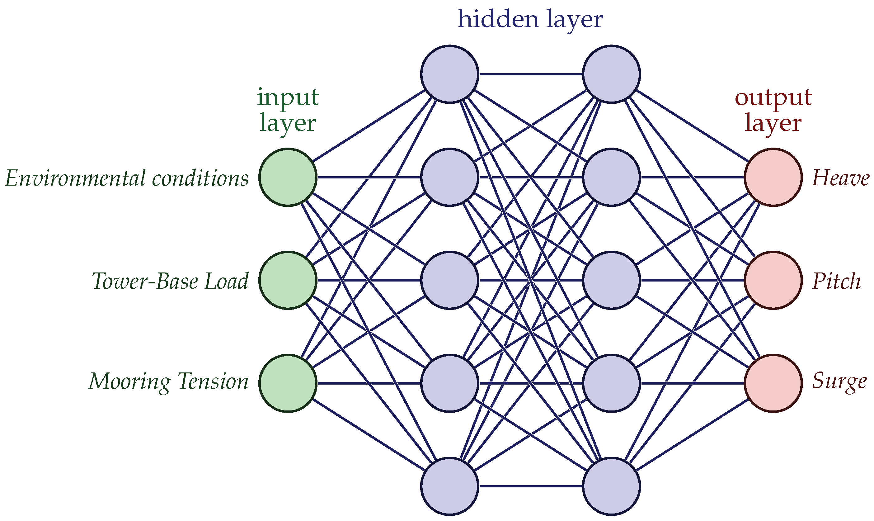
We rigorously validated the model, as depicted in Figure 1, using real-world experimental data from the OC5 Lc4.1 load case. This choice—focusing on the most complex scenario featuring combined wind and wave disturbances—demonstrates the model’s high reliability and practical utility in addressing the most demanding challenges in floating offshore wind turbine dynamics.

2. Materials and Methods

2.1. Training and Testing Data

The input data utilized in this study were collected from the global OC5 (Offshore Code Comparison Collaboration, Continued, with Correlation) experimental project. The data provided a comprehensive, multi-source data corpus detailing the stability and dynamic response of the OC5 floating wind turbine reference platform. This large-scale, multi-laboratory experimental effort ensures the dataset is robust and representative of real-world physical phenomena.

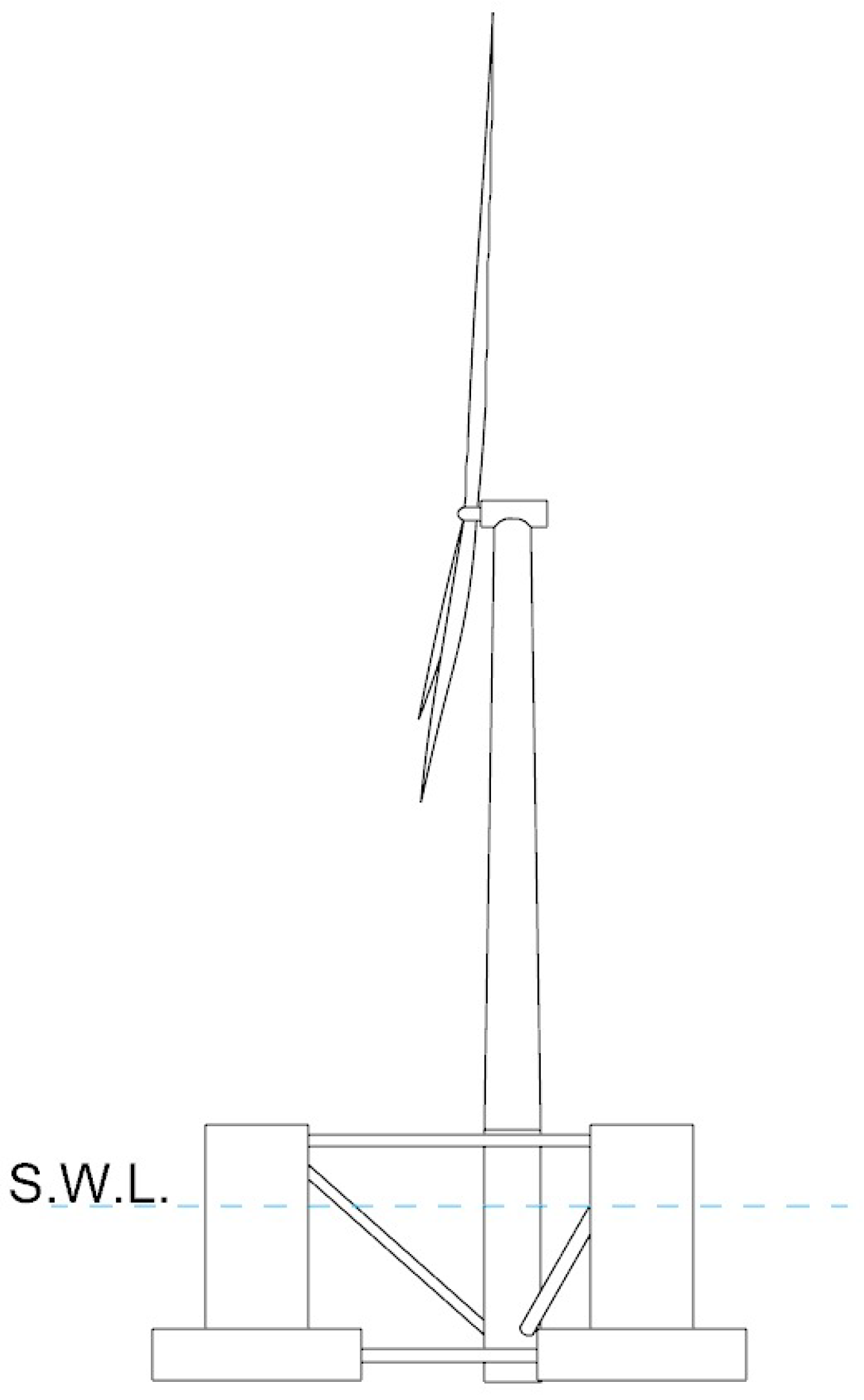
As illustrated in Figure 2, the support platform consists primarily of a central column supporting the turbine, three offset outer columns, and connecting pontoons. Platform stability and restoring forces are maintained by a three-line catenary mooring system. The primary characteristics of this reference platform are detailed in

Table 1. OC5 FoWT structural properties.

Property Name	Value
Mass	$1.3958\times {10}^7$ kg
Draft	20.0 m
Displacement	$1.3917\times {10}^4$ m3
CM location below SWL	8.07 m
Roll inertia about system CM	$1.3947\times {10}^{10}$ kg · m2
Pitch inertia about system CM	$1.5552\times {10}^{10}$ kg · m2
Yaw inertia about system CM	$1.3692\times {10}^{10}$ kg · m2

(still water line [S.W.L.]).

The dataset contains high-fidelity time-series measurements of both environmental inputs—wind speed and wave elevation—and system responses—platform motion and structural loads.

Load Case Selection

The experimental campaign encompassed a series of load cases (LC) designed to evaluate the platform’s dynamic response across various environmental conditions. These cases are categorized based on the nature of the environmental forcing, as summarized in

Table 2. Description of load cases.

Load Case	Description	Rpm	Blade Pitch (Deg)	Wave Condition	Wind Condition
4.1	Oper. Wave Steady Wind 1	12.1	1.2	Irregular: $H_s=7.1$ m, $T_p=12.1$ s, $\gamma =2.2$, JONSWAP	$V_{hub,x}=12.91$, $V_{hub,z}=-0.343$${\sigma }_x=0.5456,{\sigma }_z=0.2376$
4.2	Oper. Wave Steady Wind 2	12.1	15.0	Irregular: $H_s=7.1$ m, $T_p=12.1$ s, $\gamma =2.2$, JONSWAP	$V_{hub,x}=21.19$, $V_{hub,z}=-0.600$${\sigma }_x=0.9630,{\sigma }_z=0.4327$
4.3	Oper. Wave Dynamic Wind	12.1	1.2	Irregular: $H_s=7.1$ m, $T_p=12.1$ s, $\gamma =2.2$, JONSWAP	NPD spectrum, $\mu =13.05$
4.4	Design Wave Steady Wind 1	12.1	1.2	Irregular: $H_s=10.5$ m, $T_p=14.3$ s, $\gamma =3.0$, JONSWAP	$V_{hub,x}=12.91$, $V_{hub,z}=-0.343$${\sigma }_x=0.5456,{\sigma }_z=0.2376$
4.5	White N. Wave Steady Wind 1	12.1	1.2	White noise: $H_s=10.5$ m, $T_{range}=6-26$ s	$V_{hub,x}=12.91$, $V_{hub,z}=-0.343$${\sigma }_x=0.5456,{\sigma }_z=0.2376$

:

For the development and training of the system identification model, Load Case Lc4.1 was specifically selected. This choice was deliberate, as Lc4.1 represents a fully coupled dynamic scenario featuring simultaneous steady wind speed and irregular wave elevation as disturbances. By training the neural network on these complex, stochastic data, the model is required to learn the fundamental nonlinear mappings and inertial effects necessary to predict the platform’s motion under realistic environmental forcing.

The remaining four experimental datasets are utilized to validate the trained model’s performance across varying wind and wave intensities. This validation process ensures the model’s ability to generalize beyond its training set. The assessment is conducted through a dual-domain approach: a quantitative comparison of time-series prediction errors to evaluate temporal accuracy, and an analysis of the power spectral density (PSD) to verify that the model captures the correct frequency-domain energy distribution of the platform’s response.

2.2. Artificial Neural Networks for System Identification

An artificial neural network is a mathematical structure composed of interconnected layers: an input, one or more hidden layers, and an output layer. The network establishes an implicit, nonlinear relationship between the input and output data. The relationship between the layers is illustrated in Figure 1.

During the training phase, input data are processed by neurons. Information passes from one neuron to the next, weighted by specific parameters. The training process is an optimization task that involves adjusting the weights ($\omega$) and biases (b) associated with each layer to minimize the difference between the network’s predicted output and the target output.

The typical learning process is feedforward, meaning the output values from a previous layer are passed forward as input to the subsequent layer. Let $x_i^{(l-1)}$ be the i-th input from the previous layer $(l-1)$, ${\omega }_{ji}^{\left(l\right)}$ be the weight connecting the i-th neuron in layer $(l-1)$ to the j-th neuron in layer l, and $b_j^{\left(l\right)}$ be the bias for the j-th neuron in layer l. The total input, or pre-activation value, $a_j^{\left(l\right)}$ for the j-th neuron in layer l is

$$a_j^{\left(l\right)}=\sum _{i=1}^{n_{l-1}}{\omega }_{ji}^{\left(l\right)}{x}_i^{(l-1)}+b_j^{\left(l\right)},$$

(1)

where $n_{l-1}$ is the number of neurons in the $(l-1)$ layer. The actual output $x_j^{\left(l\right)}$ of the neuron is then determined by applying an activation function $f(·)$ to the pre-activation value:

$$x_j^{\left(l\right)}=f\left(a_j^{\left(l\right)}\right)=f\left(\sum _{i=1}^{n_{l-1}}{\omega }_{ji}^{\left(l\right)}{x}_i^{(l-1)}+b_j^{\left(l\right)}\right).$$

(2)

The activation function introduces the necessary nonlinearity into the network, enabling it to model complex, nonlinear systems. By repeating this process across all designed layers, the network produces the final estimation, $z_k$.

The network utilizes an error correction method, typically the backpropagation algorithm coupled with an optimization routine like gradient descent, to iteratively adjust the weights and biases. The ultimate objective of the training is to minimize a loss function, most commonly the mean squared error (MSE). The MSE for the output layer is calculated as

$$\mathrm{MSE}={\displaystyle \frac{1}{m}}\sum _{k=1}^m{(z_k-t_k)}^2,$$

(3)

where m is the number of output samples, $z_k$ is the network’s estimated output, and $t_k$ is the target output.

The convergence speed and predictive accuracy of the neural network are significantly influenced by the scale and distribution of the input data. In floating wind turbine systems, the dynamic response is governed by stochastic environmental forcing from wind and waves, which often results in input and output variables spanning several orders of magnitude. To ensure numerical stability and prevent features with larger absolute ranges from disproportionately influencing the weight updates, the data must be normalized. For architectures utilizing min–max normalization, the dataset is scaled to the range of [−1, 1] using the following transformation:

$$\widehat{x}={\displaystyle \frac{2(x-x_{min})}{x_{max}-x_{min}}}$$

(4)

where $\widehat{x}$ represents the normalized value, and $x_{min}$ and $x_{max}$ denote the minimum and maximum values within the specific dataset, respectively. This pre-processing step ensures that the gradients remain within a functional range, facilitating more efficient backpropagation.

To ensure the model generalizes well to unseen environmental conditions and to mitigate the risk of overfitting, a robust data-splitting strategy was implemented. The experimental dataset was partitioned into three distinct subsets: a training set (70%), a validation set (15%), and a test set (15%). The training subset is used exclusively for the iterative adjustment of the network’s weights and biases. The validation set serves as an independent monitor during the learning process; it is used to evaluate the model’s generalization capability and to trigger early stopping if the validation error begins to diverge, thereby preventing the model from memorizing noise in the training data. Finally, the test set is reserved for an unbiased assessment of the optimized network’s performance, providing a definitive measure of the system identification model’s accuracy in predicting coupled 3-DOF motions.

3. Results and Discussion

In this section, the impact of varying the hyperparameters of the artificial neural network on its performance is discussed. Specifically, the relationship between the network’s performance metrics and the structural complexity, defined by the number of neurons within the hidden layers and the number of hidden layers itself, will be investigated.

To determine the impact of neural network architecture and tuning techniques on predictive accuracy, a backpropagation neural network was implemented using the MATLAB Neural Network Toolbox. The optimization of the model’s performance was primarily driven by refining the network structure, specifically the configuration of hidden layers and neurons. The baseline hyperparameters and training configurations utilized for this study are summarized in

Table 3. Hyperparameter settings and system environment for the neural network.

Category	Parameter	Values/Setting
Model structure	Input features	WindVxi, WindVzi, WaveElev
		TwrBsFxt, TwrBsFyt, TwrBsFzt
		TwrBsMxt, TwrBsMyt, TwrBsMzt
		Fair1Ten, Fair2Ten, Fair3Ten
	Output	3 DOFs (Heave, Pitch, Surge)
	Hidden Layers	[2–15, 2–15] nodes
	Activation function	Hyperbolic tangent (tansig)
	Input Normalization	Min–Max normalization to [−1, 1]
	Epochs	1000
Training setup	Optimizer	Levenberg–Marquardt (trainlm)
	Loss function	Mean Squared Error
	Learning rate	0.01
Learning strategy	Performance Goal	$1\times {10}^{-6}$
	Data split (train/validation/test)	0.70/0.15/0.15
	Software Framework	MATLAB 2024b
System environment	CPU	Apple M4 Pro (12-core)
	RAM	24 GB

. These settings represent the standard environment used to ensure consistent convergence and prevent overfitting during the training phase.

3.1. Metrics for Model Evaluation

To rigorously evaluate the performance and complexity of the trained neural network model, three widely used regression metrics are introduced: the root mean squared error (RMSE), the mean absolute error (MAE), and the coefficient of determination (${\mathrm{R}}^2$).

The root mean squared error (RMSE) is defined as the square root of MSE. RMSE is particularly useful because the error is expressed in the **same units as the target variable. Furthermore, due to the squaring of the errors, RMSE penalizes large errors more than small errors. This characteristic makes it a suitable metric when large deviations from the target value are considered especially critical in the system.

$$\mathrm{RMSE}=\sqrt{{\displaystyle \frac{1}{m}}\sum _{k=1}^m{(z_k-t_k)}^2},$$

(5)

The mean absolute error (MAE) calculates the average magnitude of the errors by taking the absolute difference between the prediction and the target. Since MAE uses the absolute value, it provides a linear measure of the error magnitude. This linearity makes the metric more robust to outliers compared to RMSE, as outliers do not disproportionately inflate the overall error value. Consequently, MAE offers a clear interpretable average error expressed directly in the original units.

$$\mathrm{MAE}={\displaystyle \frac{1}{m}}\sum _{k=1}^m|z_k-t_k|,$$

(6)

The coefficient of determination, ${\mathrm{R}}^2$, quantifies the proportion of the variance in the dependent variable that is predictable from the independent variables. It is a measure of model fit.

$${\mathrm{R}}^2=1-{\displaystyle \frac{S{S}_{\mathrm{res}}}{S{S}_{\mathrm{tot}}}},$$

(7)

where $S{S}_{\mathrm{res}}$ is the sum of squares of the residuals:

$$S{S}_{\mathrm{res}}=\sum _{k=1}^m{(z_k-t_k)}^2,$$

(8)

and $S{S}_{\mathrm{tot}}$ is the total sum of squares (proportional to the variance of the data), defined using the mean of the target values, $\overline{t}$:

$$S{S}_{\mathrm{tot}}=\sum _{k=1}^m{(t_k-\overline{t})}^2,\mathrm{with}\overline{t}={\displaystyle \frac{1}{m}}\sum _{k=1}^m{t}_k.$$

(9)

${\mathrm{R}}^2$ provides a standardized score, typically ranging from 0 to 1, which makes it an excellent measure to understand the overall effectiveness of the model regardless of the scale of the target variable. A value close to 1 indicates that the model explains a high proportion of the variance in the data, signifying a strong fit.

3.2. Sensitivity Analysis of Neural Networks

Determining the optimal complexity of the artificial neural network is crucial to avoid both underfitting and overfitting. To analyze the influence of network architecture on model performance, a sensitivity analysis was performed by systematically varying the number of hidden layers and the number of neurons within them. The performance evaluation metrics introduced in Section 3.1 (RMSE, MAE, and ${\mathrm{R}}^2$) were utilized for this analysis [15].

The investigation primarily focused on two structural variations:

• Increasing the number of neurons in a single hidden layer (e.g., 1(2) to 1(15)).
• Comparing a single layer to a two-layer structure with equivalent total complexity (e.g., 1(8) vs. 2(4-4)).

3.2.1. Effect of Neuron Count

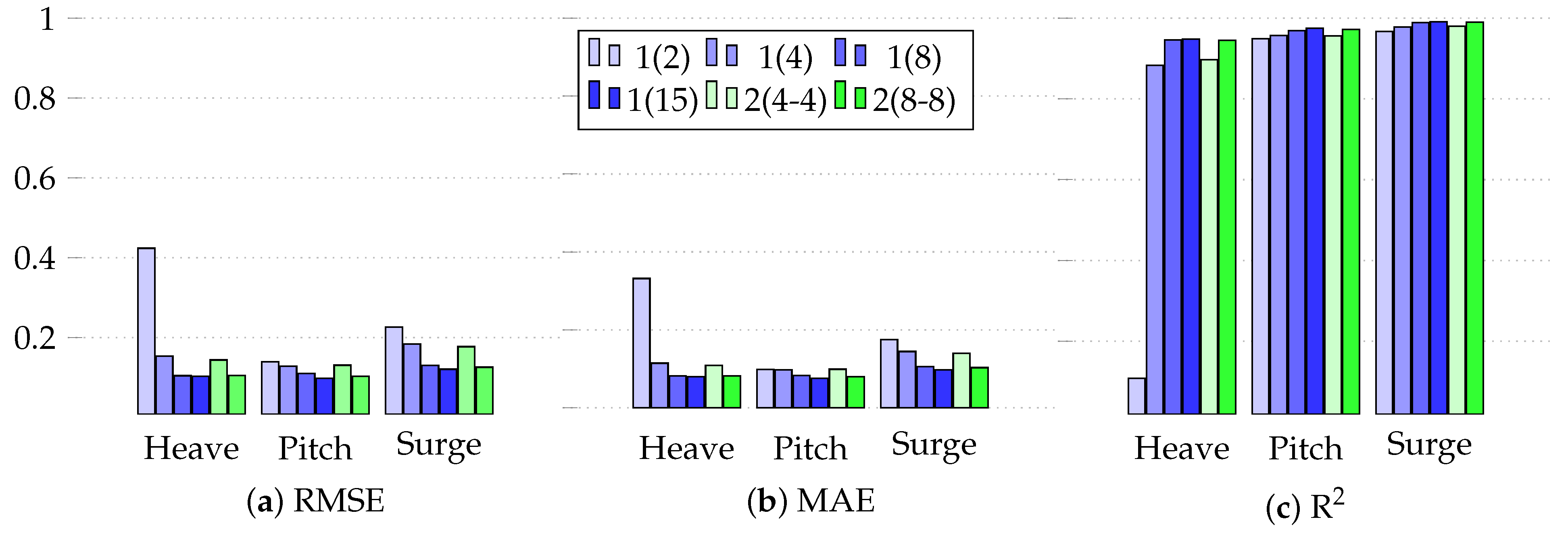
Increasing the number of neurons within a single hidden layer generally improved the predictive capability of the network. The prediction errors (RMSE and MAE) and the coefficient of determination (${\mathrm{R}}^2$) for various configurations are summarized in

Table 4. Performance metrics for different neural network architectures.

Architecture	Root Mean Squared Error			Mean Absolute Error			Coefficient of Determination
Layers (Neurons)	Heave (m)	Pitch (Deg)	Surge (m)	Heave (m)	Pitch (Deg)	Surge (m)	Heave (m)	Pitch (Deg)	Surge (m)
1(2)	0.424	0.139	0.226	0.332	0.098	0.175	0.108	0.949	0.967
1(4)	0.153	0.128	0.184	0.114	0.097	0.144	0.883	0.957	0.978
1(8)	0.104	0.110	0.130	0.082	0.083	0.106	0.946	0.969	0.989
1(15)	0.103	0.098	0.121	0.080	0.075	0.097	0.948	0.975	0.991
2(4-4)	0.144	0.131	0.177	0.108	0.099	0.140	0.897	0.956	0.980
2(8-8)	0.105	0.103	0.126	0.081	0.079	0.103	0.945	0.972	0.990

and Figure 3.

A significant performance gain is observed when increasing the configuration from 1(2) to 1(8) neurons. However, further expanding the hidden layer to 15 neurons yields diminishing returns. Specifically, the improvement in RMSE for the 1(15) configuration relative to the 1(8) configuration is minor, registering $1.69\%$, $12.48\%$, and $7.84\%$ reductions in error for the Heave, Pitch, and Surge motion predictions, respectively, indicating that 1(8) neurons are near the point of optimal complexity for this specific single-layer architecture.

3.2.2. Effect of Hidden Layer Depth

Comparison between single- and double-layer networks, such as the 1(8) and 2(4-4) configurations, showed that the single-layer design was generally superior or equivalent. For instance, the 2(4-4) configuration exhibited similar or slightly reduced performance compared to 1(8) (Table 4), suggesting that increasing the depth does not offer a performance advantage over increasing the width for this specific system identification task.

3.3. Performance of Prediction Model

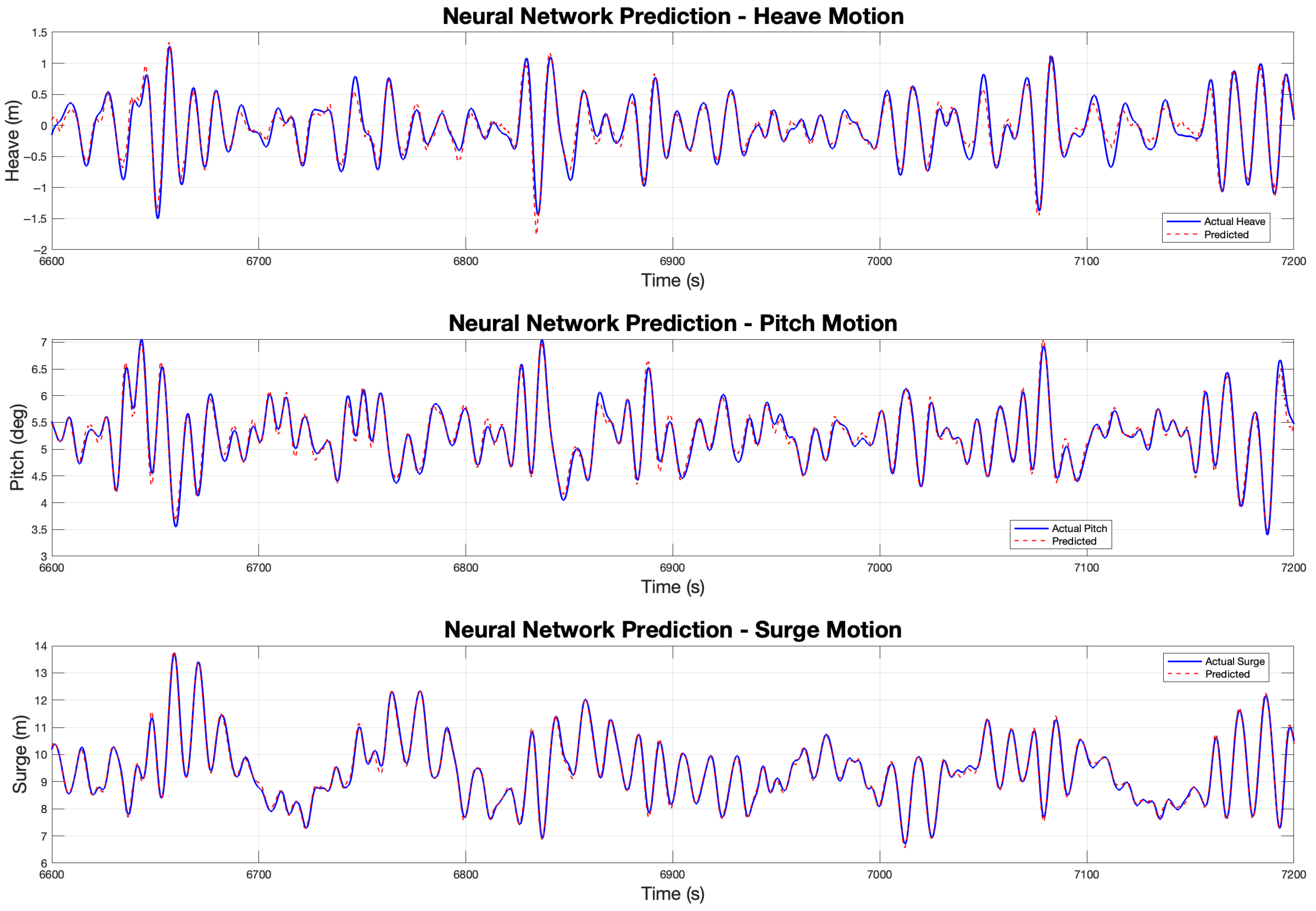
The predictive performance of the trained neural network model across the three coupled degrees of freedom, Heave, Pitch, and Surge, is qualitatively assessed by comparing the model’s output against experimental measurements over a representative test interval (t = 6600 s to t = 7200 s).

As illustrated in Figure 4, the figure demonstrates exceptionally high predictive fidelity. The predicted signal trace (red dashed line) is virtually superimposed upon the actual experimental data (blue line) across the full time window for all three coupled motions.

For the analysis of this nonlinear dynamic system, the NN maintains superior phase coherence. Crucially, the model exhibits no discernible time lag or phase shift between the predicted and actual responses across the entire test window. This confirms the NN’s capacity to accurately capture the system’s high-frequency temporal dependencies and inertial effects, providing strong evidence that the network has successfully learned the causal relationships governing the platform’s dynamics.

Furthermore, the network achieved excellent amplitude tracking across highly non-stationary environmental conditions. It accurately predicted large-magnitude excursions, including Surge peaks exceeding $1.4$ m and Pitch peaks near $7.0^{\circ }$, as well as small-amplitude oscillations. This performance validates the model’s ability to capture nonlinear hydrodynamic and aerodynamic forces across the entire operating envelope.

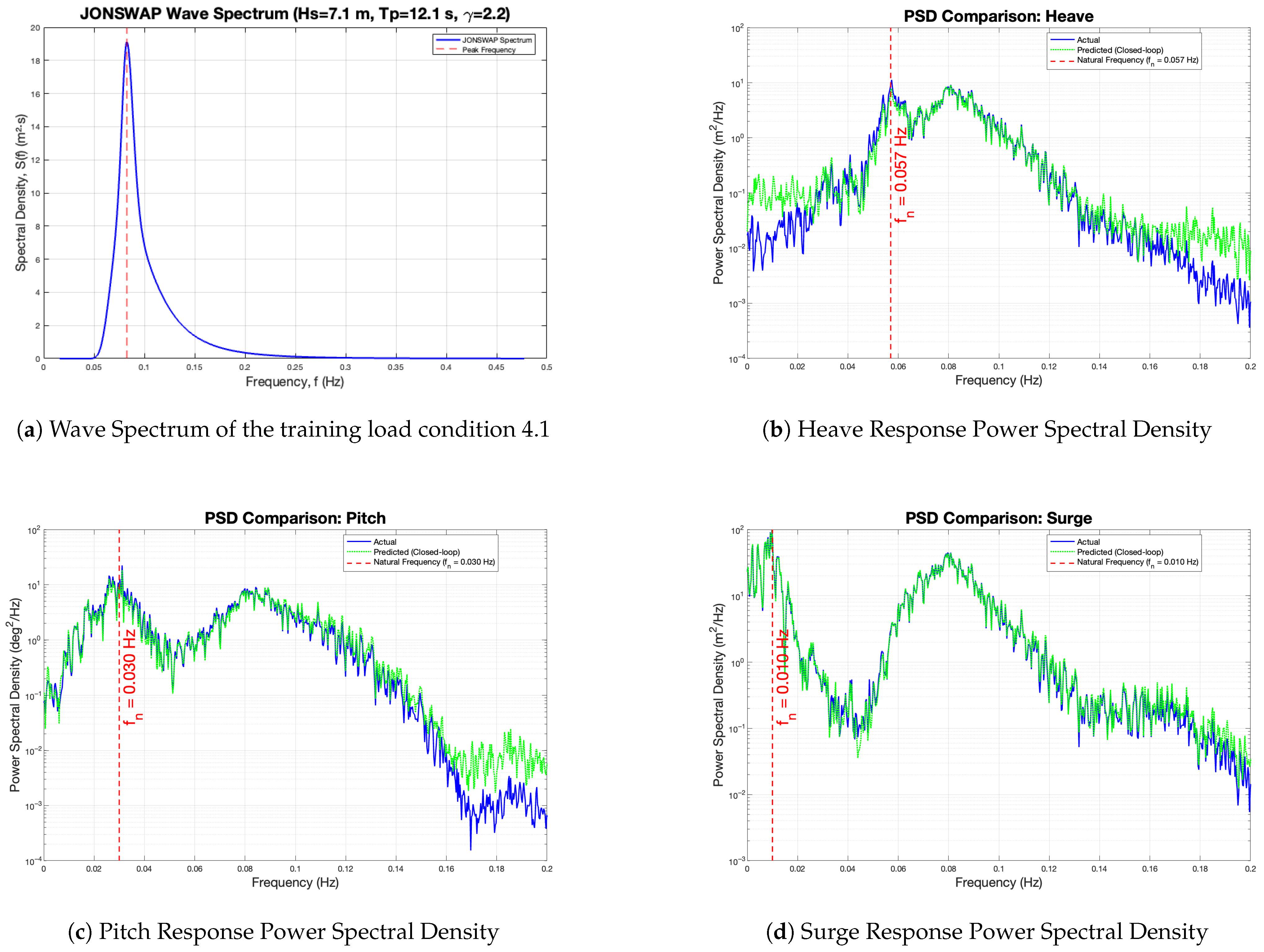
To verify that the model captures the underlying physics of the floating system beyond simple time-step matching, the response was analyzed in the frequency domain using power spectral density. The analysis was specifically tailored to the 0–0.2 Hz frequency range, as the input wave spectrum indicates that this region contains the primary wave energy and governs the first-order wave excitations. As shown in Figure 5, the NN model accurately reproduces the spectral energy distribution and successfully identifies the system’s natural frequencies for Heave, Pitch, and Surge. The precise alignment of the spectral peaks demonstrates that the data-driven model has implicitly learned the eigenfrequencies and resonant characteristics, ensuring that the predicted motions are physically consistent with the stochastic wave environment of the OC5 campaign.

The simultaneous, high-fidelity tracking observed in both the time and frequency domains confirms that the ANN successfully emulated the complex interactions governing the 3-DOF system response, establishing it as an effective, high-fidelity surrogate model for FOWT global dynamics.

3.4. Generalization Performance Across Heterogeneous Load Cases

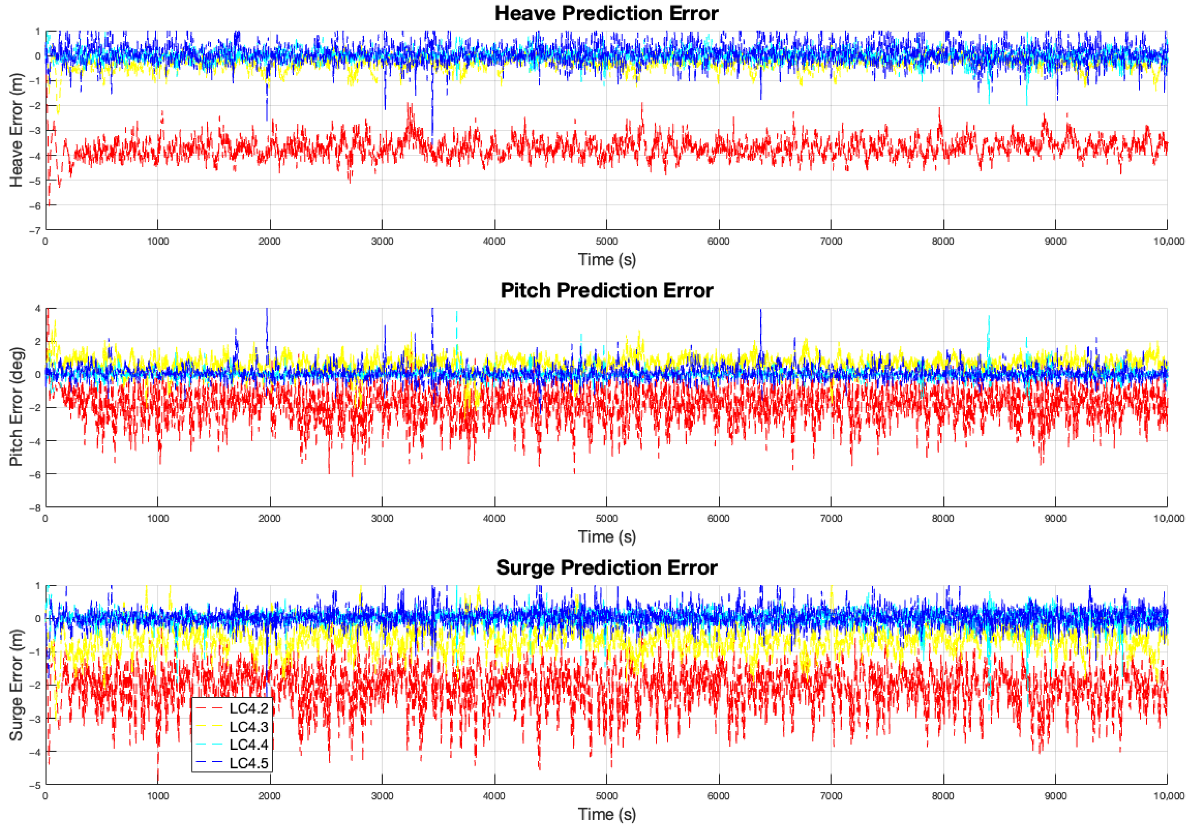
To evaluate the robustness and generalization capability of the trained FNN, the model was deployed to predict the platform dynamics for the remaining experimental scenarios, Load Cases 4.2 through 4.5. These cases introduce significant environmental variations, including fluctuating wind speeds, turbulent wind profiles, and diverse irregular wave spectra.

As illustrated in Figure 6, the model demonstrates a strong ability to generalize the system’s dynamic patterns. In most scenarios, the predicted time series closely tracks the experimental measurements. However, a notable phenomenon was observed in Load Case 4.2, which involves a change in the mean wind speed. While the FNN accurately identified the oscillation frequencies and periodic patterns, a discernible shift in the response magnitude, characterized by a mean offset, was present across all three degrees of freedom. This suggests that while the network has mastered the hydrodynamic restoration and wave-frequency mapping, the sensitivity to step changes in aerodynamic thrust requires further calibration.

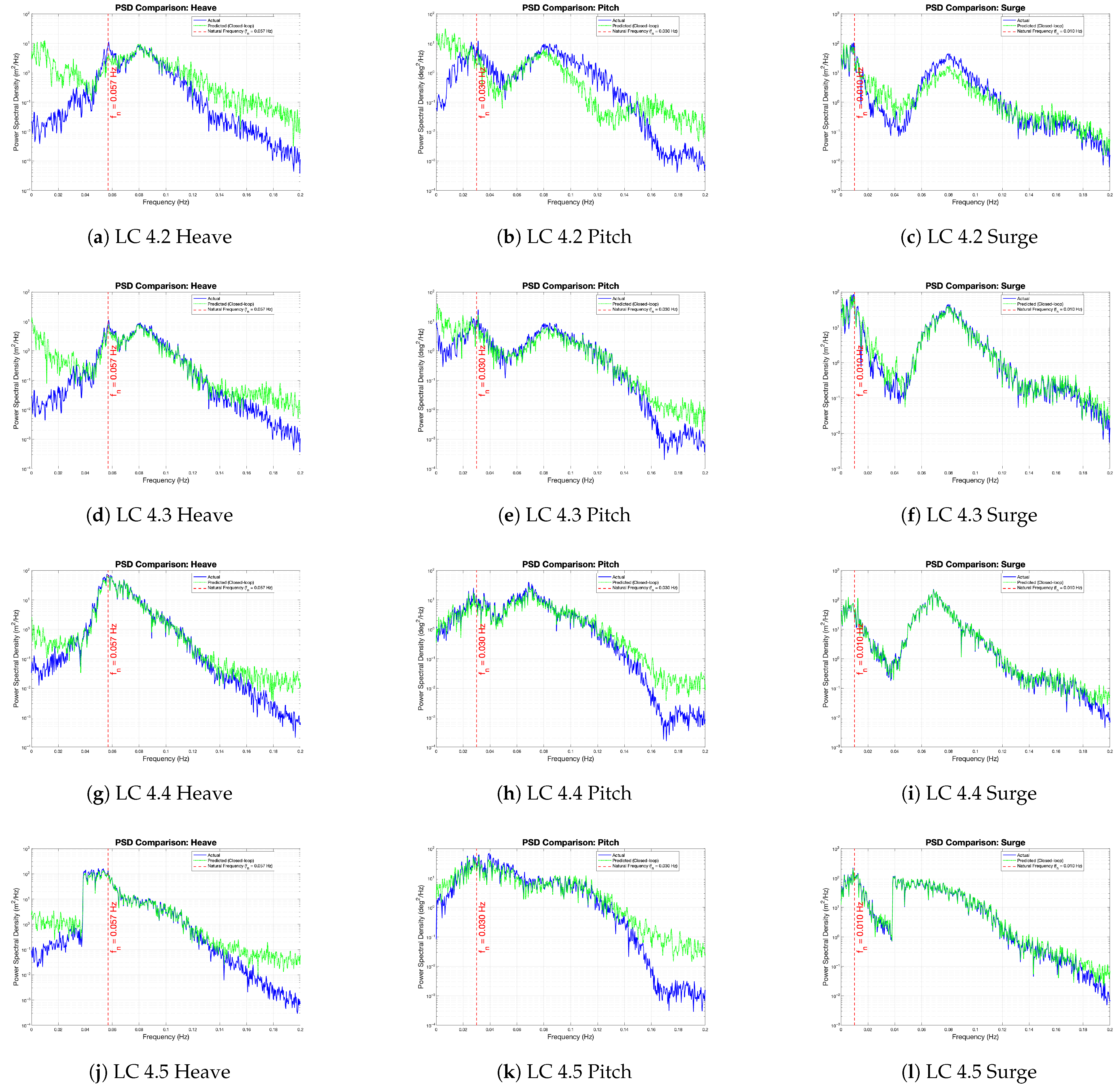
Furthermore, the model’s frequency-domain performance was assessed across the complex scenarios (LC 4.3–4.5), which include fully stochastic wind and wave forcing. Figure 7 presents the combined power spectral density for these cases. The spectral analysis reveals that the model maintains high fidelity in estimating energy distribution even under irregular environmental loading. The alignment of the spectral peaks suggests that the FNN is particularly robust in adapting to varied wave conditions. These results indicate that, while the current model serves as a highly effective surrogate for wave-induced dynamics, the “gap” in predicting varying wind-strength magnitudes remains an area for future investigation. This likely stems from the training set (LC 4.1) containing a single steady wind speed, limiting the network’s exposure to the thrust-curve nonlinearities present in LC 4.2.

4. Conclusions

This study successfully demonstrated the utility of an optimized feedforward neural network as a high-fidelity surrogate model for the complex, nonlinear system identification of floating offshore wind turbines. By leveraging real-world experimental data from the demanding OC5 model, the developed NN model achieved a prediction capability that was visually and quantitatively superior.

The analysis of the time-domain results confirmed that the network achieved exceptionally high predictive fidelity, characterized by superior phase coherence and accurate amplitude tracking across all three coupled degrees of freedom. This qualitative assessment is supported by the quantitative results, which consistently show an exceptionally high coefficient of determination for the most challenging motions. This low error magnitude confirms that the NN effectively learned the underlying causal dynamic relationships and inertial effects governing the platform’s response.

The successful implementation of this methodology introduces a novel, computationally efficient tool for the offshore wind industry. The trained NN provides near-instantaneous, high-accuracy predictions. The necessity for such a model is driven by the critical requirement to accurately capture large-amplitude, nonlinear dynamic behaviors—as observed in wave tank experiments—within a computationally feasible framework. These efficient simulations are essential for evaluating platform stability and safety during extreme sea states where linear approximations fail to account for higher-order hydrodynamic effects. This capacity is particularly significant for applications requiring rapid analysis, such as Real-Time Digital Twinning, Accelerated Design and Optimization, and Onboard Condition Monitoring.

This research represents a technical progression from our group’s foundational work in advanced system identification. Previous studies primarily utilized the Reverse-Multiple Input Single Output (R-MISO) technique, a frequency-domain spectral method, for parameter estimation (e.g., extracting frequency-dependent damping coefficients) to correct and refine physics-based potential flow models of ships and wave energy devices [16,17]. The current work differs fundamentally by transitioning to a fully data-driven, non-parametric approach. Here, the FNN acts as a direct surrogate model, bypassing the need for explicit physics equations. Furthermore, this study complements our group’s previous investigations into the long-term probabilistic survival of FOWTs, extending those efforts by providing a means to rapidly assess extreme response statistics under stochastic loading conditions [18,19]. This progression demonstrates the growing maturity and robustness of purely data-driven methods to handle the full, nonlinear complexity of coupled 3-DOF FOWT dynamics in the time domain, a task previously reliant on semi-empirical hybrid techniques.

Despite the overall high fidelity, evaluating the model across distinct load cases revealed specific boundaries in its generalization capability. The FNN demonstrated robust performance when predicting responses under varied and irregular wave conditions, confirming its mastery of the system’s hydrodynamic restoration and wave-frequency mapping. However, a noticeable performance gap emerged in scenarios with changed wind conditions, specifically in Load Case 4.2. In these instances, while the model successfully captured the oscillation frequencies and periodic patterns, it exhibited a magnitude shift in the predicted response. This limitation likely stems from the training data (LC 4.1), which was characterized by steady wind conditions. Consequently, the model lacked the exposure to the nonlinear aerodynamic thrust curves and mean drift variations present in turbulent or changing wind environments, identifying a critical requirement for more diverse training datasets to achieve universal predictive accuracy.

This research provides two main take-home messages. First, feasibility of data-driven methods in offshore engineering: The high-fidelity performance achieved with real experimental data validates the introduction of data-driven neural network methods into the offshore industry, establishing a pathway toward smarter and more efficient design, analysis, and operation of FOWTs. Second, predictive excellence in complex dynamics: The optimized FNN architecture is fully capable of serving as a surrogate model for highly nonlinear, coupled dynamic systems, achieving an accuracy level previously reserved for advanced physics-based solvers.

Future research will focus on creating a hybrid, multi-scale prediction framework to leverage the strengths of both spectral and data-driven methods. Specifically, we intend to apply the R-MISO method as an auto-encoder for frequency domain analysis. By analyzing the Fast Fourier Transform (FFT) data, R-MISO can extract fundamental modal information about the long-term dynamic characteristics and systemic properties of the OC5 platform. These long-term features will then be combined as additional, physics-informed inputs to the neural network. This hybrid approach yields a predictive model capable of both instantaneous, high-frequency response prediction and robust tracking of long-term structural trends. Consequently, it enhances predictive accuracy and physical interpretability across all operational timescales.