Genotype by Environment Interaction for Growth in Atlantic Cod (Gadus morhua L.) in Four Farms of Norway

Abstract

We studied genotype by environment interaction (G × E) for body weight (BW) of Atlantic cod (Gadus morhua L.) from the National cod breeding program in Norway. Records of 13,811 fish in a nucleus farm (NUC) and two test farms (PE_North, PE_South) in year-class (YC) 2007, and for 9149 fish in NUC and one test farm in YC 2010 were available. Heterogeneity of variances and heritabilities ($h^2$) were estimated using a univariate animal model with environmental effects common to full-sibs (full-model). Genetic correlations ($r_g$) between farms were estimated using a multivariate full-model and a reduced-model (without $c^2$) for each YC. Heterogeneity of $h^2$ was observed in both YC 2007 (0.10 to 0.16) and YC 2010 (0.08 to 0.26). The estimates of $r_g$ between NUC and test farms were relatively high for both models (0.81 ± 0.19 to 0.96 ± 0.17) and (0.81 ± 0.08 to 0.86 ± 0.04), suggesting low re-ranking of genotypes. Strong re-ranking of genotypes between PE_South and PE_North may be less important because most cod producers are situated close to the breeding nucleus. In conclusion, G × E between NUC and test farms were low and at present there is no need for separate breeding programs for BW in cod.

1. Introduction

Growth defined as body weight (BW) at harvest is an economically important trait in Atlantic cod (Gadus morhua L.) and other aquaculture species. In Norway, cod is produced in open-sea cages in the fjords from north to south with wide ranges of farming conditions and environmental variations (e.g., temperature, photoperiod and management practices). The existing family-based National cod breeding program (Nofima, Tromsø) supplies genetically improved juveniles to commercial farms in different parts of Norway. In aquaculture, environmental variables such as photoperiod, temperature and production system may significantly influence growth performance of fish across production environments [1]. Differences in the environmental variables may induce a phenomenon called genotype by environment interaction (G × E).

The G × E can be separated into two forms: re-ranking and heterogeneity of variances. Re-ranking means that the rank order of genotypic performance change across different environments [2], i.e., the best genotypes in one production environment may not be the best in other production environments [3]. The degree of re-ranking can be quantified by genetic correlations ($r_g$) between fish from the same families reared in two different environments, treating measurements at each environment as a separate trait [3]. If the $r_g$ differs from unity, it indicates the presence of re-ranking [3]. Consequently, selection based on one environment may reduce genetic gain in other production environments [4]. The heterogeneity of variances refers to the change in the magnitude of the additive genetic variance for a trait across different environments. In most studies in plants, magnitude of additive genetic variance tends to be larger in optimal environments than in suboptimal environments [5]. However, several laboratory studies in animals have shown both higher and lower heritabilities in optimal environments [6].

A previous study of G × E in Atlantic cod by Kolstad et al. [7] reported weak re-ranking ($r_g$ = 0.82 to 0.95) for two-year body weight measured in different locations off the coast of Norway. However, Kolstad et al., (2006) did not include common environmental family effects, which can be quite large (9% of total phenotypic variation) [8]. Also, body weight at two-year is a less relevant selection criteria than at 2.5 years of age, as used in the current selection criteria, as it can be highly influenced by the sexual maturation status of fish [9]. Furthermore, the G × E may vary for different traits among the species and different populations within the species depending on the trait and farm environments, and should be studied on a case-by-case basis [10,11]. Therefore, the objective of the current study was to quantify the magnitude of G × E for BW of Atlantic cod from the Norwegian National cod breeding program, reared at the breeding nucleus and three other environments, by estimating genetic correlations and heterogeneity of variances.

2. Materials and Methods

2.1. Fish Materials

All fish used in this study were produced in the nucleus breeding facility at the National cod breeding program (Nofima, Tromsø, Norway). The wild-caught brood-fish used to form the base population originated from distinct genetic groups, namely, coastal cod and north-east Arctic cod [12,13]. Furthermore, coastal cod was divided into coastal cod south and coastal cod north based on geographical origin [8,14]. Eggs and milt from base parents were stripped and fertilized to create year-class (YC) 2003, 2004 and 2005 as distinct parent generations (P1). The P1 generation was purebred, whereas later YC were purebred as well as crosses between the three genetic groups. In the present study, two year-classes were used, YC 2007 and YC 2010. The YC 2007 was produced as first generation (F1) using selected parents from YC 2004. Later, selected parents from YC 2007 were used to produce YC 2010 as a second generation (F2). The fish have been selected mainly for growth, defined as body weight (BW) after two summers at sea (2.5 years of age), but in some year classes, also for vibriosis (a bacterial disease caused by Vibrio anguillarum) resistance [8]. A hierarchical mating design was followed (with few exceptions) where in most cases each sire was mated with two dams, while each dam was mated with one sire. However, mortality and poor performance in the hatchery and start feeding resulted in many unsuccessful matings and few half-sib families. Some sires and dams were re-used across year-classes to create genetic links between the year-classes. Hence, YC 2007 also had some selected parents from other parallel P1 (i.e., YC 2003). All families were produced during a two-month period (March to April) in both years (2007 and 2010) and reared separately until individual tagging with Passive Integrated Transponders (PIT, Sokymat, Switzerland) tags (September to October, 2007 and 2010) at the age of 198 to 212 days. The stocking densities at the larval rearing in individual family tanks were similar. However, due to difference in survival rate within each family until tagging, some families ended up with more survivors compared to others. Fifty fish per family were randomly selected and PIT-tagged for grow out at the nucleus farm (NUC) and 25 fish per family were PIT-tagged for grow out at each of the test farms. Tagged fish were conditioned in a single tank and transferred to open sea-cage farms (March to April in 2008 and in 2011) for the growth performance study. The NUC was used for both year-classes whereas PE_North and PE_South were used for YC 2007 and PE_Mid was used for YC 2010. All fish were fed commercial cod dry pelleted feed. In total, 22960 fish from 379 full-sib and half-sib families (273 sires and 367 dams) were recorded for growth at four different farms. Descriptive statistics of the data used in the analyses are given in the Table 1.

Table 1. Descriptive statistics of growth data from family groups of Atlantic cod at four farms in Norway.

Year class	Farms	Fish, no	Family, no	Sires, no	Dams, no	Fish per Family			TWT, g		TAG, day		AG, day		BW, g
						Mean	Min	Max	Mean	s.d.	Mean	s.d.	Mean	s.d.	Mean	s.d.
2007	NUC	10,685	185	140	185	57	4	112	27	9	205	3	977	9	2431	600
	PENorth	924	155	125	155	6	1	15	27	9	205	2	959	6	2414	582
	PESouth	2202	141	116	141	15	5	45	28	9	205	2	966	7	1880	442
2010	NUC	6977	193	132	180	36	12	79	26	8	202	2	945	10	2715	569
	PEMid	2172	178	127	167	12	1	21	26	8	202	2	998	9	3365	673
All farms		22,960	379	273	367				28	9	204	3	966	19	2552	680

TWT = weight at tagging; TAG = age at tagging; AG = age at registration; BW = body weight; s.d. = standard deviation.

Table 1. Descriptive statistics of growth data from family groups of Atlantic cod at four farms in Norway.

Year class	Farms	Fish, no	Family, no	Sires, no	Dams, no	Fish per Family			TWT, g		TAG, day		AG, day		BW, g
						Mean	Min	Max	Mean	s.d.	Mean	s.d.	Mean	s.d.	Mean	s.d.
2007	NUC	10,685	185	140	185	57	4	112	27	9	205	3	977	9	2431	600
	PENorth	924	155	125	155	6	1	15	27	9	205	2	959	6	2414	582
	PESouth	2202	141	116	141	15	5	45	28	9	205	2	966	7	1880	442
2010	NUC	6977	193	132	180	36	12	79	26	8	202	2	945	10	2715	569
	PEMid	2172	178	127	167	12	1	21	26	8	202	2	998	9	3365	673
All farms		22,960	379	273	367				28	9	204	3	966	19	2552	680

TWT = weight at tagging; TAG = age at tagging; AG = age at registration; BW = body weight; s.d. = standard deviation.

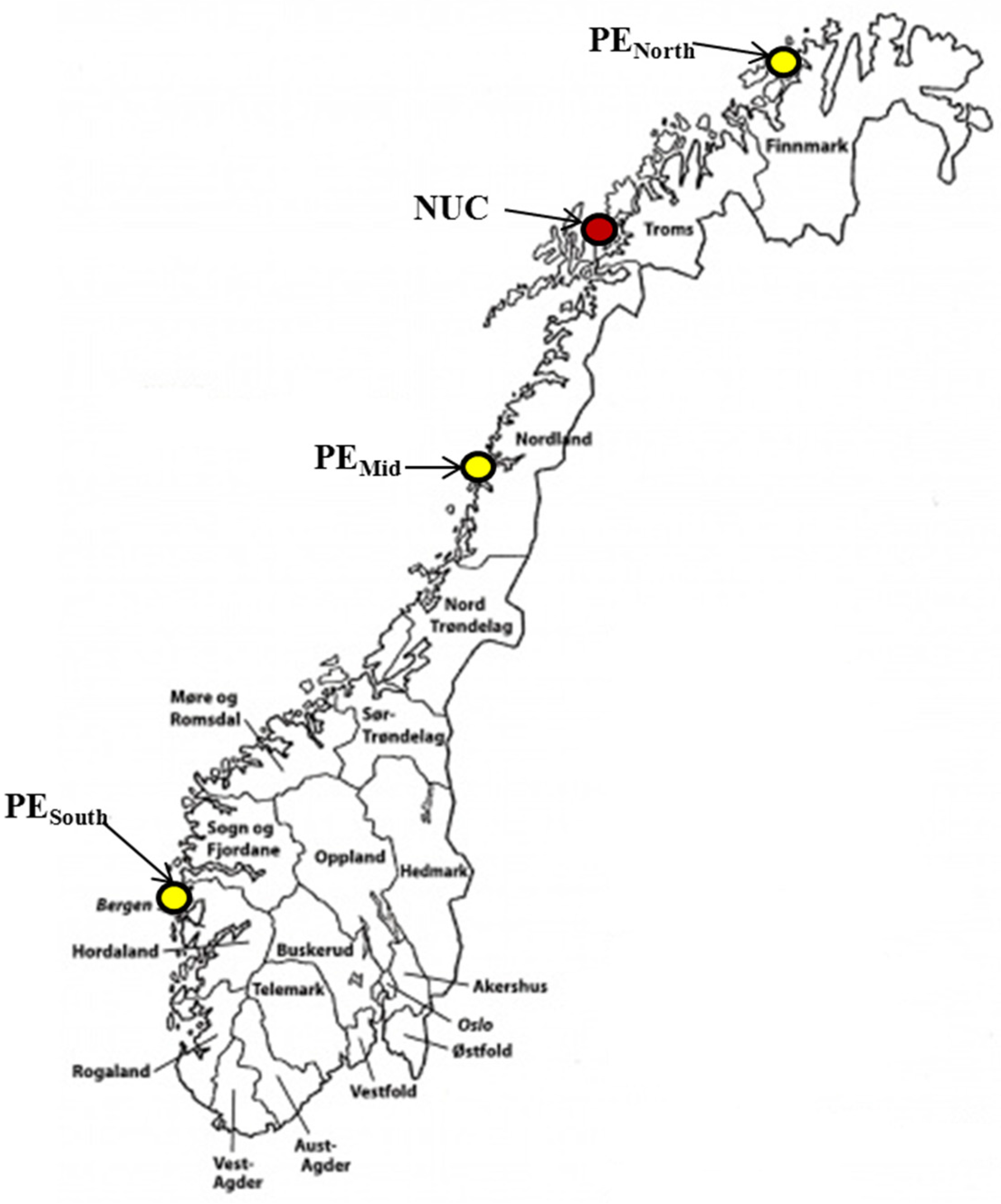
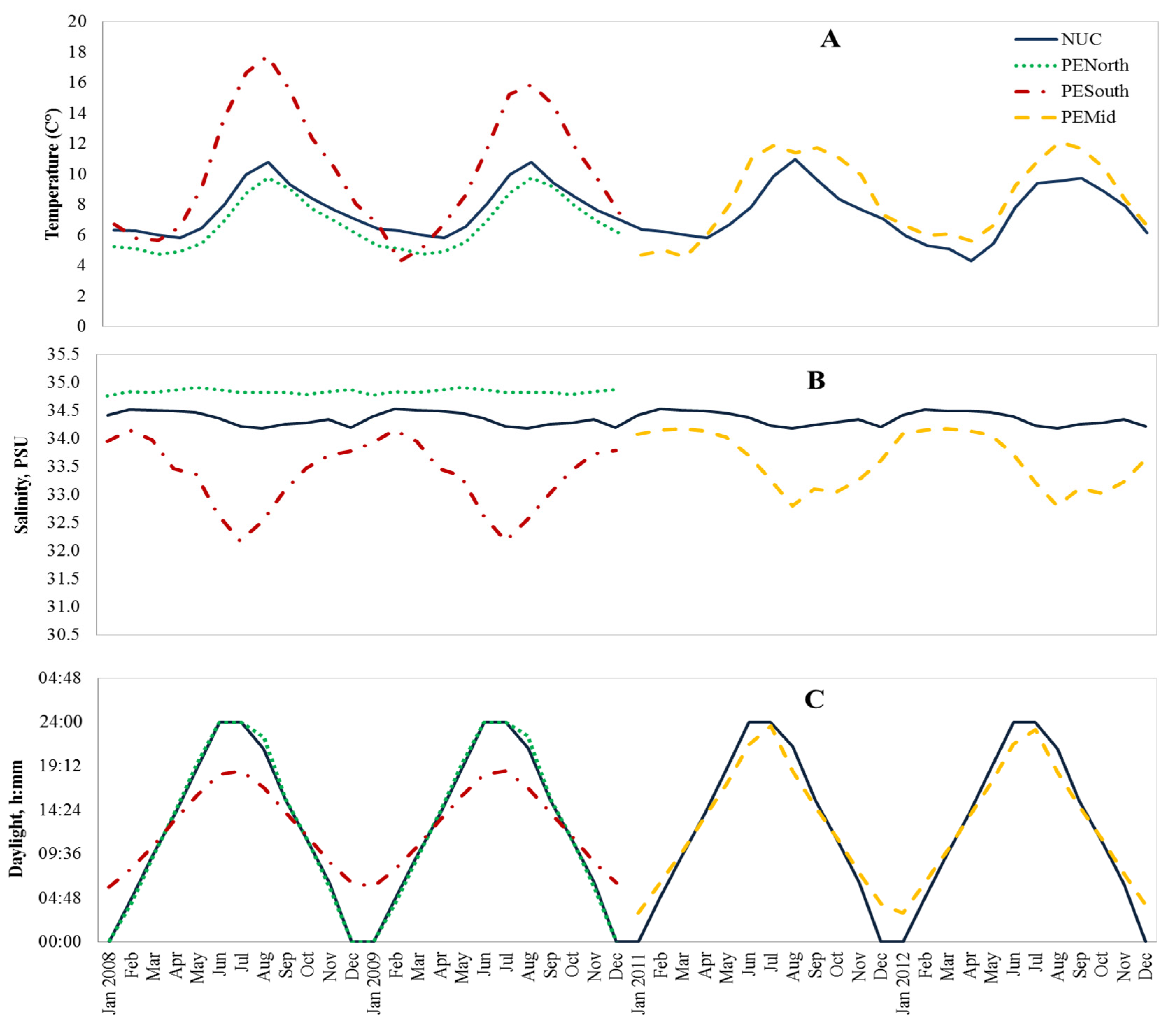
2.2. Test Environments

The fish were grown at four sea-cage farms at different geographical locations and under different production conditions (Figure 1.). The farm NUC at Røsnes Ringvassøy, Tromsø (approx. 70° N, 19° E) belongs to nucleus breeding facility. The PE_North at Lebesby in northern Norway (approx. 71° N, 27° E) was chosen as a representative of commercial production environment. The PE_South and PE_Mid are aquaculture research facilities at Austevoll in southwestern Norway (approx. 60° N, 5° E) and Helgeland in northern Norway (approx. 66° N, 13° E), respectively.

Figure 1. Location of grow out environments in Norway.

Figure 1. Location of grow out environments in Norway.

The major differences between the four different farms with respect to environmental variables were photoperiod and temperature (Figure 2). At NUC and PE_North, sea surface temperature varied from 4.3 °C to 11 °C and 3.8 °C to 9.9 °C, respectively. Due to the extreme latitude, locations in both of these farms experience polar days during summer (20 June, with 24:00 h of daylight) and polar night during winter (21 December, with 0:00 h of daylight). In contrast, the sea surface temperature in Farms PE_South and PE_Mid varied from 3.8 °C to 17.8 °C and 4.6 °C to 13 °C, respectively. In addition, in both PE_South and PE_Mid, length of daylight was similar and varied throughout the year; 20 June with approximately 18:45 h of day light and 21 December with approximately 6:00 h of daylight (Figure 2). Average monthly sea surface salinity (PSU) and sea surface temperature (°C) were obtained using MyOcean global ocean observation-based products (V3.1), and data was extracted using QGIS (v2.4.0). Photoperiod (hours:minutes of daylight) was obtained from data made available by the United States Naval Observatory (USNO) [15]. In addition to these factors, PE_North was a commercial farm whereas the other farms were research centers. However, the type of feed, feeding regime and other management practices followed across these farms were similar.

Figure 2. Environmental factors on the four farms: (A) average monthly sea surface temperature (degrees Celsius, °C); (B) average monthly salinity (practical salinity units, PSU); and (C) hours and minutes of day light (first day of the month).

Figure 2. Environmental factors on the four farms: (A) average monthly sea surface temperature (degrees Celsius, °C); (B) average monthly salinity (practical salinity units, PSU); and (C) hours and minutes of day light (first day of the month).

2.3. Data Collection

At each farm, fish were grown for 945 to 998 days post hatching (approximately 2.5 years of age) until they reached commercial harvest size. On harvesting day, fish were screened individually for PIT-tags using a PIT-tag reader and corresponding BW was recorded to the nearest 10 grams using a digital balance. Also, sex of the fish was determined using Ultrasound by stage of gonadal development [16]. The total production volume in YC 2007 at NUC, PE_North and PE_South was 26.0, 2.5 and 4.13 metric tons, respectively. Likewise, production volume in YC 2010 was 19.0 metric tons at NUC and 7.3 metric tons at PE_Mid.

2.4. Statistical Analyses

The data preparation and descriptive statistics calculations were carried out using SAS statistical software [17]. The potential significance of fixed effect (sex) and linear covariates (age at harvest and heterosis) on BW was tested using the software ASReml V3 [18]. Heterosis for each fish was defined as either being crossbred (1) or purebred (0) based on from which population the fish originated. Age at harvest (AGE) and heterosis was used to correct for variation in age and population effect, respectively. For each farm, only the significant effects (P < 0.05) were fitted in the model for the genetic analysis.

The BW recorded in each YC from different farms was considered as separate genetic traits and both univariate and multivariate analyses was performed. Variance-covariance components were estimated using restricted maximum likelihood (REML) in mixed animal models using ASReml V3 [18].

2.4.1. Univariate Analysis

The univariate analysis was performed to estimate heterogeneity of variances and heritability ($h^2$). In addition, the significance of environmental effects common to full-sibs was tested in the univariate analysis by comparing two models: the model with environmental effects common to full-sibs (full-model as shown below) or without environmental effects common to full-sibs (reduced-model):

$$y_{}= X\text{β}+Z_{1}a+Z_{2}c+e$$

where, $y$ is the vector of individual BW measurements from each farm, $\text{β}$ is the vector of fixed effects, $a$ is the vector of additive genetic random effects, $c$ is the vector of random environmental effects common to full-sibs and $e$ is the vector of random residual effects. It was assumed that random variables ($a$ , $c$ and $e$) are normally distributed. Specifically, $\text{a}~\text{N}\left(0,{\text{Aσ}}_a^2\right)$ , where ${\text{σ}}_a^2$ is the additive genetic variance and $\text{A}$ is the additive genetic relationship matrix derived from the pedigree traced back to the base population; $\text{c}~\text{N}\left(0,{\text{Iσ}}_c^2\right)$ , where ${\text{σ}}_c^2$ is the common environmental variance; $\text{e}~\text{N}\left(0,{\text{Iσ}}_e^2\right)$ , where ${\text{σ}}_e^2$ is the residual variance and $\text{I}$ is the identity matrix. The $X$ , $Z_1$ and $Z_2$ are the design matrices assigning observations to the levels of fixed effects, additive genetic effects, and environmental effects common to members of the each full-sib family, respectively. Omitting significant family components may lead to the over estimation of genetic variance and inflated heritability estimates. The effect of overall mean and sex was fitted for all four farms, whereas, the effect of AGE was fitted as a regression term for NUC (both YC 2007 and 2010) and PE_South. Finally, the effect of heterosis was fitted as a regression term for NUC (both YC 2007 and 2010), PE_North and PE_Mid.

The full-model was compared with the reduced-model using likelihood ratio test (LRT) [2,18] to test for the significance of environmental effects common to full-sibs. The test statistic equals two times the absolute difference between log-likelihoods (lnL) of full-model (Lf) and reduced model (Lr). For a single variance component, the theoretical asymptotic distribution of the LRT is a mixture of chi-square (${\chi }^2)$ distributions, where mixing probabilities are 0.5, with 0 and 1 degrees of freedom [19]. Mathematically,

$$\text{LRT}=-2\left[\ln \left(L_r\right)-\ln \left(L_f\right)\right]~{\chi }_{df=0and1,\text{ α}=0.05}^2$$

The approximate P-value for LRT statistic is $0.5 (1-\text{Pr}(~{\chi }_{1 }^2\le d$)) where d is the calculated value of LRT statistic. This has a 5% significance critical value of 2.71.

2.4.2. Multivariate Analysis

Re-ranking was assessed by calculating $r_g$ using a multivariate model with the same fixed and random effects as in the univariate analysis and by treating individual BW recorded at each farm as separate traits. The analysis was performed separately for each YC. Thus, data from YC 2007 (NUC, PE_North and PE_South) and YC 2010 (NUC and PE_Mid) was analyzed using tri-variate and bivariate analysis, respectively. Since an individual fish was present at one farm only, the residual covariance between farms was set to zero. Because the estimates of genetic correlation and common environmental full-sib family correlation in the full-model had high standard errors of the estimate in most of the farms, the analysis was performed using both the reduced-model and the full model.

2.4.3. Calculation of Genetic Parameters

For each trait, heritability ($h^2$) was calculated as:

$$h^2=\frac{{\sigma }_a^2}{{\sigma }_a^2+{\sigma }_c^2+{\sigma }_e^2}$$

where ${\text{σ}}_a^2$ , ${\text{σ}}_c^2$ (only for full-model) and ${\text{σ}}_{\text{e}}^2$ are additive genetic variance, environmental variance common to full-sibs, and residual variance, respectively. Correspondingly, the fraction of phenotypic variance explained by common environmental family effects ($c^2$) was calculated as:

$$c^2=\frac{{\text{σ}}_c^2}{{\text{σ}}_a^2+{\text{σ}}_c^2+{\text{σ}}_e^2}$$

Heterogeneity of variances across farms was compared by estimating phenotypic [$C{V}_p$ = (${\text{σ}}_p$/$\overline{X}$) × 100], genetic [$C{V}_a$ = (${\text{σ}}_a$/$\overline{X}$) × 100] and residual [$C{V}_e$ = (${\text{σ}}_e$/$\overline{X}$) × 100] coefficients of variation (CV) [20]. Where, ${\text{σ}}_p$ , ${\text{σ}}_a$ and ${\text{σ}}_e$ are phenotypic, genetic and residual standard deviations, respectively. The $\overline{X}$ is the phenotypic mean for BW measured in different farms. The $C{V}_a$ was preferred over ${\text{σ}}_a^2$ to compare the degree of heterogeneity of genetic variances across farms because it is unaffected by the trait mean changes across farms.

The r_g between BW measured at two different farms was calculated as [3]:

$$r_g=\frac{{\text{σ}}_{aE1,aE2}}{\sqrt{{\text{σ}}_{aE1}^2\times {\text{σ}}_{aE2}^2}}$$

where $r_g$ is the correlation coefficient between additive genetic values (predicted breeding values), ${\text{σ}}_{aE1,aE2}$ is the covariance between additive genetic values measured at farm E1 and E2, ${\text{σ}}_{aE1}^2$ and ${\text{σ}}_{aE2}^2$ is the additive genetic variance of BW measured in one farm (E1) and the other farm (E2). In the full-model, the common environmental full-sib family correlation between two farms was calculated as:

$$r_c=\frac{{\text{σ}}_{cE1,cE2}}{\sqrt{{\text{σ}}_{cE1}^2\times {\text{σ}}_{cE2}^2}}$$

where $r_c$ is the correlation coefficient between common environmental full-sib family effects, ${\sigma }_{cE1,cE2}$ is the covariance between full-sib family effects, ${\sigma }_{cE1}^2$ and ${\sigma }_{cE2}^2$ is the full-sib family variance of BW measured in one farm (E1) and the other farm (E2).

3. Results

3.1. Descriptive Statistics

The phenotypic mean of BW for YC 2007 was highest in NUC (2431 g) followed by PE_North (2414 g) and PE_South (1880 g) (Table 1). For YC 2010, PE_Mid had higher mean BW (3365 g) compared to NUC (2715 g). The fish recorded at PE_Mid were 53 days older at the time of harvest compared to the fish at NUC.

3.2. Heterogeneity of Genetic Variation

The magnitudes of $C{V}_p$ in YC 2007 for NUC (23.21), PE_North (23.13), and PE_South (22.30) were similar (Table 2). Likewise, the magnitudes of $C{V}_p$ in YC 2010 for NUC (20.37) and PE_Mid (19.82) were similar. For YC 2007, the largest ${\text{σ}}_a^2$ was observed in NUC (50,498) followed by PE_North (31,634) and PE_South (21,675) (Table 2). However, $C{V}_a$ for NUC (9.24) was similar to PE_North (7.37) and PE_South (7.83), suggesting that the differences in ${\text{σ}}_a^2$ were mostly due to trait mean differences. For YC 2010, ${\text{σ}}_a^2$ was higher for NUC (78,629) than for the test farm PE_Mid (34,401). The ${\text{σ}}_a^2$ differed between the farms, indicating that heterogeneity of variances was present, which was supported by different magnitudes of $C{V}_a$ . The $C{V}_a$ for NUC (10.33) was approximately two-folds higher compared to PE_Mid (5.51).

Table 2. Estimates of phenotypic (${\text{σ}}_p^2$), additive genetic (${\text{σ}}_a^2$), and residual (${\text{σ}}_e^2$) variance, phenotypic ($C{V}_p$), additive genetic ($C{V}_a$), and residual coefficient of variance ($C{V}_e$), heritability ($h^2$) and environmental variance common to full-sibs ($c^2$) with their corresponding standard errors (s.e.) for body weight (BW) of Atlantic cod in different farms.

Year-class	Farm	${\sigma }_p^2$	${\sigma }_a^2$	${\sigma }_e^2$	$C{V}_p$	$C{V}_a$	$C{V}_e$	$h^2$ ± s.e.	$c^2$ ± s.e.*
2007	NUC	318,420	50,498	247,060	23.21	9.24	20.45	0.16 ± 0.06	0.07 ± 0.02
	PENorth	311,780	31,634	249,250	23.13	7.37	20.68	0.10 ± 0.10	0.10 ± 0.05
	PESouth	175,840	21,675	134,460	22.30	7.83	19.50	0.12 ± 0.09	0.11 ± 0.04
2010	NUC	305,970	78,629	205,300	20.37	10.33	16.69	0.26 ± 0.07	0.07 ± 0.03
	PEMid	444,830	34,401	375,410	19.82	5.51	18.21	0.08 ± 0.06	0.08 ± 0.03

* Bold letters indicates significant effects of common environment tested using likelihood ration test (LRT) $~ {\chi }^2$ with 0 and 1 degrees of freedom, α = 0.05.

Table 2. Estimates of phenotypic (${\text{σ}}_p^2$), additive genetic (${\text{σ}}_a^2$), and residual (${\text{σ}}_e^2$) variance, phenotypic ($C{V}_p$), additive genetic ($C{V}_a$), and residual coefficient of variance ($C{V}_e$), heritability ($h^2$) and environmental variance common to full-sibs ($c^2$) with their corresponding standard errors (s.e.) for body weight (BW) of Atlantic cod in different farms.

Year-class	Farm	${\sigma }_p^2$	${\sigma }_a^2$	${\sigma }_e^2$	$C{V}_p$	$C{V}_a$	$C{V}_e$	$h^2$ ± s.e.	$c^2$ ± s.e.*
2007	NUC	318,420	50,498	247,060	23.21	9.24	20.45	0.16 ± 0.06	0.07 ± 0.02
	PENorth	311,780	31,634	249,250	23.13	7.37	20.68	0.10 ± 0.10	0.10 ± 0.05
	PESouth	175,840	21,675	134,460	22.30	7.83	19.50	0.12 ± 0.09	0.11 ± 0.04
2010	NUC	305,970	78,629	205,300	20.37	10.33	16.69	0.26 ± 0.07	0.07 ± 0.03
	PEMid	444,830	34,401	375,410	19.82	5.51	18.21	0.08 ± 0.06	0.08 ± 0.03

* Bold letters indicates significant effects of common environment tested using likelihood ration test (LRT) $~ {\chi }^2$ with 0 and 1 degrees of freedom, α = 0.05.

There were indications of heterogeneous $h^2$ estimates which varied from 0.10 ± 0.10 to 0.16 ± 0.06 for YC 2007 (in three farms) and 0.08 ± 0.06 to 0.26 ± 0.07 for YC 2010 (two farms) (Table 2). However, the differences for YC 2007 were relatively small and for both YC the standard errors were quite large. The lowest $h^2$ estimates were observed in PE_North and PE_Mid and were due to the lower ${\text{σ}}_a^2$ but higher ${\text{σ}}_c^2$ and ${\text{σ}}_e^2$ , compared with the NUC. In addition, $c^2$ was significant (p < 0.05) for all farms in both YC, indicating that some effects common to full-sibs are beyond additive genetic control. In addition, based on LRT test statistic, the full-model was the best fit in all farms in the univariate analysis.

3.3. Genetic Correlations

Genetic correlations between BW recorded at the breeding nucleus (NUC) and at the test farms PE_North, PE_South and PE_Mid are given in Table 3. The magnitude of $r_g$ from the full-model and the reduced-model were similar, but differed in terms of accuracy of the estimates. Genetic correlations estimated using the reduced-model for BW between NUC and others test farms (PE_North, PE_South and PE_Mid) were 0.81 ± 0.08 to 0.86 ± 0.04, indicating re-ranking of families between NUC and test farms (Table 3). Although high $r_g$ (0.81 ± 0.19 to 0.96 ± 0.38) and moderate to high $r_c$ (0.68 ± 0.18 to 0.77 ± 0.12) were estimated using the full-model between NUC and test farms, the estimates were less accurate than when using the reduced model indicated by high standard errors of the estimates. In YC 2007, the $r_g$ between the two test farms (PE_North and PE_South) was moderate (0.63 ± 0.11) from reduced-model and highly inaccurate (0.07± 0.65) from full-model. The full-sib family effects appear to capture and artificially reducing the genetic covariance between PE_North and PE_South.

Table 3. Estimates of genetic (above diagonal) and common environmental correlations (below diagonal for full-model) for body weight (BW) in Atlantic cod. Estimates ± s.e.

	Full-model a				Reduced-model a
Farms	NUC	PENorth	PESouth	PEMid	PENorth	PESouth	PEMid
NUC		0.92 ± 0.38	0.96 ± 0.17	0.81 ± 0.19	0.81 ± 0.08	0.86 ± 0.04	0.84 ± 0.05
PENorth	0.68 ± 0.18		0.07 ± 0.65	-		0.63 ± 0.11	-
PESouth	0.77 ± 0.12	0.84 ± 0.15		-			-
PEMid	0.69 ± 0.23	-	-

^a Animal mixed model with (full-model) or without (reduced-model) environmental effects common to full-sibs in trivariate and bivariate settings for the data from YC 2007 (NUC, PE_North and PE_South) and YC 2010 (NUC and PE_Mid), respectively.

Table 3. Estimates of genetic (above diagonal) and common environmental correlations (below diagonal for full-model) for body weight (BW) in Atlantic cod. Estimates ± s.e.

	Full-model a				Reduced-model a
Farms	NUC	PENorth	PESouth	PEMid	PENorth	PESouth	PEMid
NUC		0.92 ± 0.38	0.96 ± 0.17	0.81 ± 0.19	0.81 ± 0.08	0.86 ± 0.04	0.84 ± 0.05
PENorth	0.68 ± 0.18		0.07 ± 0.65	-		0.63 ± 0.11	-
PESouth	0.77 ± 0.12	0.84 ± 0.15		-			-
PEMid	0.69 ± 0.23	-	-

^a Animal mixed model with (full-model) or without (reduced-model) environmental effects common to full-sibs in trivariate and bivariate settings for the data from YC 2007 (NUC, PE_North and PE_South) and YC 2010 (NUC and PE_Mid), respectively.

4. Discussion

The main finding in our study was that there was low evidence of re-ranking of genotypes (families) in test farms with respect to BW, which is the primary trait selected for in the breeding nucleus. However, G × E in terms of heterogeneity of genetic variances between the farm environments were present. In addition, heterogeneous $h^2$ estimates were observed across some of the farm environments.

4.1. Genotype by Environment Interaction

The magnitude of the $r_g$ (0.81 to 0.96) across YC suggested low re-ranking of genotypes (families) for BW between NUC and test farms (Table 3). The magnitude of $r_g$ estimates from reduced-model was comparatively lower but more accurate than the full-model which also included a common environmental family effect. Although it is not possible to deduce the exact $r_g$ , it is safe to conclude that the actual estimate of $r_g$ may be more than 0.81 between the estimates of reduced-model and full-model. The individual fish families were reared in a separate tank but with similar common environmental conditions until they were tagged (~222 days) and this could also the reason for low G × E (low re-ranking) observed in our study. A similar study in Atlantic cod by Kolstad et al. [7] also reported re-ranking $(r_g$ = 0.82 to 0.95) for two year BW measured in different locations off the coast of Norway and concluded that BW in Atlantic cod may be sensitive to environmental changes. In contrast to the study of Kolstad et al. [7], a larger number of full-sib families (>100 vs. 51) and common environmental family effects were used in the present study and BW was measured at approximately 2.5 vs. 2 years of age. At 2.5 years of age, the cod are closer to the commercial harvest size and the body weight is likely to be less affected by sexual maturation status of the fish [9]. There are a number of studies in different species the have generally reported the absence of significant G × E for growth traits [21]. For example, in salmonids, low G × E was reported for BW when families were reared in different locations off Norway [22,23]. In GIFT tilapia (Oreochromis niloticus), Khaw et al. [24] concluded that G × E for growth related traits $(r_g$ = 0.73 to 0.85) between different pond and cage environment was unimportant. In the same species, $r_g$ (0.63 to 0.95) estimates for harvest BW suggested moderate to negligible re-ranking across different test ponds [25]. Nevertheless, there are studies, for example, in common carp (Cyprinus carpio), where significant G × E for growth related traits have been reported [26]. Although G × E for BW in European sea bass (Dicentrarchus labrax) was absent [27], but was significant for growth related trait such as growth rate defined as daily growth coefficient [11].

In YC 2007, PE_North and PE_South had low $r_g$ with high standard errors of the estimate (Table 3). Apart from sampling errors, environmental differences could have been the reason for weak $r_g$ , as these farms were far apart geographically, leading to large differences in day light and sea surface temperature (Figure 2). Generally, G × E is expected to be more prominent with more differences in farming conditions. For example, a recent study by Sae-Lim et al. [20] revealed strong re-ranking and significant G × E for growth related traits for rainbow trout (Oncorhynchus mykiss) grown in different countries and continents with very different environmental conditions. All four farms used in our study varied with respect to photoperiod and temperature throughout the year. Furthermore, the farms with the largest differences in photoperiod and sea surface temperature (PE_North and PE_South) had the lowest $r_g$ compared to the other farms (Table 3). The effect of photoperiod and genotype [28], and temperature and population [29,30] on growth of Atlantic cod has been demonstrated earlier.

In our study, there were indications of heterogeneous additive genetic variances and $h^2$ between farms (Table 2). In aquaculture breeding program, performance of selection candidates situated in a breeding nucleus and sibs from test farms can be treated as separate genetic traits in the genetic evaluation which automatically accounts for heterogeneity of variances between farms [31]. The presence of substantial $C{V}_a$ in each farm (Table 2) also suggested the potential for selecting BW in NUC using sib performance data from test farms. However, the existence of genetic heterogeneity of environmental variance in each farm (environment) may also affect the phenotypic variance (phenotype) [32]. This has been demonstrated in Atlantic salmon [33] and rainbow trout [34], but has not been studied in detail for BW in Atlantic cod. The magnitude of additive genetic and environmental components explaining total phenotypic variation for a particular trait can vary with environmental conditions and $h^2$ may change accordingly [35]. The differences in the amount of ${\text{σ}}_a^2$ present resulted in the difference in the h2 across farms (Table 2). The moderate h2 estimates (0.16 to 0.26) observed in NUC are in agreement with earlier studies using the data from the same farm [8,36]. In general, similar $h^2$ estimates were reported for growth related traits in tilapia [37], European seabass [27] and other species [21]. The $c^2$ effect was substantial across farms (0.07 to 0.11) and should be accounted for in the genetic analysis to get unbiased estimates of genetic parameters and increased accuracy of selection [25]. Previously, Bangera et al. [8] also reported substantial c² effect (0.08) using the subset of data from NUC. Both potential dominance genetic effects and common environmental effect caused by the separate rearing of full-sib families until tagging and maternal effects are included in the c² effect. Thus, excluding c² effect may lead to the over estimation of ${\text{σ}}_a^2$ and thus biased $h^2$ and $r_g$ estimates. A study in cod by Tosh et al. [38] concluded that poor data structure and models without $c^2$ effect can potentially lead to overestimation of $h^2$ . Positive common environmental full-sib family correlations ($r_c$ = 0.68 to 0.77) between NUC and test farms supports the evidence for moderate family by farm interaction for BW (Table 3). Thus, the ranking of families with respect to growth is expected to change across farms. However, the best growing families in NUC and test farms may not be genetically the best ones because environmental correlation (i.e., $r_c$) is strongly positive. These estimates have not been estimated before for cod and positive $r_c$ indicates that the best families for growth in NUC can be taken as a good predictor of growth in test farms.

The accuracy of $h^2$ and $r_g$ estimates depends on sample size and pedigree structure and can be biased due to confounding effects caused by experimental design leading to improper partitioning of total phenotypic variance into casual sources [35]. The inaccurate h2 estimates in test farms and the low and inaccurate $r_g$ between PE_North and PE_South may also be explained by the family structure in the data. Many families had no half-sibs for which additive genetic and common environmental effects can be completely confounded except if there is some information from more distant relatives through the pedigree. Thus, environmental (and non-additive genetic) effects common to full-sibs may be present, but are difficult to separate from the additive genetic effects and could thus result in unambiguous estimate of additive genetic variance [2]. In most fish breeding programs, each sire is mated to at least two unrelated dams in a nested full-sib and half-sib designs to produce full-sib and half-sib family groups [2]. Some of the families produced at our facility were not present at tagging because of mortality after spawning and/or some of the families were excluded due to strict quality control followed at the hatchery stage. The number of individuals per family may also influence the $h^2$ and $r_g$ estimates. It has been shown that, low number of families (less than 100) and family size (less than 10) with low $h^2$ (~0.1) may result in downward biased $r_g$ estimate and incorrectly suggest that strong genotype re-ranking is present in the population [39]. Although more than 100 families were present in all farms in the present study, the number of fish per family in PE_North varied from 1 to 15. The low and imprecise $r_g$ between PE_North and PE_South (Table 3) may also be due to low $h^2$ estimates and unequal family contributions in these farms [39]. As the number of individuals per family increases, the accuracy of $h^2$ estimates will increase by means of comparably small standard errors of the estimate [40]. Therefore, with $c^2$ present in the data, better mating structure (e.g., partly factorial mating design) [41] and larger numbers of fish per family may be required to get reliable estimates of genetic parameters and breeding values. This has been reported for rainbow trout where accuracy of estimated breeding values of sea BW for selection candidates located in breeding nucleus (freshwater) increased when the number of individuals per family tested at sea farms increased (from 7 to 20 per family) [42].

4.2. Implications for Breeding

The accuracy of selection depends on the $h^2$ of the trait; high $h^2$ will lead to better accuracy and faster genetic gain, and the opposite is true with low $h^2$ [43]. Heterogeneous variances and h² observed in our study may result in differences in the accuracy of selection and predicted genetic gain for growth of cod across farms. However, G × E in the form of heterogeneity of variances and h² is often considered unimportant in aquaculture because there is usually a single breeding program for all production environments and selection candidates are usually located in a breeding nucleus. If the selection candidates are situated in different farm environments, the genetic evaluation procedure proposed by Meuwissen et al. [44] can handle heterogeneous variances across farms to get unbiased estimates of breeding values. Nevertheless, in a multiple trait index selection, heterogeneity of variances between farms can cause re-ranking of genotypes [45]. This may occur even for single trait index selection if the same trait is under different genetic control in different farms but the selection is based on information from one farm. The impact of heterogeneity of variances between farms on re-ranking of genotypes in a single trait and multiple trait index selection needs to be further investigated for fish breeding programs.

When there is a genotype re-ranking, optimization of a breeding program is recommended. Incorporating sib information from different production environment can be implemented to increased genetic gain across environments. To obtain increased understanding of the consequences of G × E, we performed deterministic simulation using SelAction software [46]. The genetic parameter estimates from the current study were used as the input. We compared two different breeding strategies: (1) selection based on information in the NUC only; and (2) selection based on information both in the NUC and information from sibs reared at different production environments. When selection in YC 2007 was based on information in the NUC only, the genetic gain was 37% lower in PE_North and 45% lower in PE_South compared to the gain in NUC. For YC 2010, the genetic gain was 45% lower in PE_Mid. Thus, selecting purely based on information in the NUC lead to significantly lower genetic gain in the production environments. When sib information from PE_North and PE_South was included in the selection index, genetic gain increased by 5%, 13% and 10% at NUC, PE_North and PE_South, respectively when all locations are assumed economically equally important in YC 2007. Similarly, for YC 2010, genetic gain increased by 1% for NUC and 7% for PE_Mid when including sib information into the selection index.

If the genotype re-ranking is very strong, a break-even $r_g$ [47] can be used as a criteria to justify establishing environment-specific breeding programs. The break-even $r_g$ is defined as the intersection of genetic correlations when the relative cost and genetic gain of different breeding programs is equal. When the $r_g$ across environments is lower than the break-even $r_g$ , separate breeding programs are recommended. In fish breeding, the break-even $r_g$ is expected to be higher, i.e., ≥0.70 [20] than in dairy cattle, i.e., 0.61 to 0.70 [47,48] of the use of sib testing in aquaculture which puts more emphasis on own performance than progeny testing. In addition, a higher break-even $r_g$ is expected in fish breeding due to the high fecundity leading to higher selection intensity [47]. Although $r_g$ between PE_North and PE_South is lower than the break-even $r_g$ , running two separate breeding programs is very costly. In addition, at present, most cod producers are situated in the north of Norway, which is close to the breeding nucleus, and there is no competition from other breeding programs. Hence, strong re-ranking between PE_North and PE_South becomes less important. Optimizing Atlantic cod breeding program by incorporating sib information [42,49] in PE_North and PE_Mid should therefore be sufficient to maintain high genetic gain across environments.

5. Conclusions

The knowledge of G × E is essential to optimize breeding programs without compromising genetic gain. Though there were indications about heterogeneous variances across farms, estimates of genetic correlations (re-ranking) between NUC and test farms (0.81 to 0.96) indicated low G × E. In contrast, strong re-ranking was observed between PE_North and PE_South (0.07 and 0.63). However, the strong re-ranking between PE_North and PE_South may be less important because, presently, most cod producers are situated in northern Norway, which is close to the breeding nucleus. Furthermore, selection for BW in the breeding nucleus is expected to yield reliable genetic gain by incorporating sib-performance data from different farms in the genetic evaluations. Therefore, we conclude that, at present, there is no need to establish additional breeding programs for improved growth rates for specific environments.

References

1. Sae-Lim, P.; Komen, H.; Kause, A.; Mulder, H.A. Identifying environmental variables explaining genotype-by-environment interaction for body weight of rainbow trout (Onchorynchus mykiss): Reaction norm and factor analytic models. Genet. Sel. Evol. 2014, 46, 16. [Google Scholar] [CrossRef] [PubMed] [Green Version]
2. Lynch, M.; Walsh, B. Genetics and Analysis of Quantitative Traits; Sinauer Associates: Sunderland, MA, USA, 1998. [Google Scholar]
3. Falconer, D.S.; Mackay, T.F. Introduction to Quantitative Genetics; Longman: New York, NY, USA, 1996. [Google Scholar]
4. Mulder, H.; Bijma, P. Effects of genotype × environment interaction on genetic gain in breeding programs. J. Anim. Sci. 2005, 83, 49–61. [Google Scholar] [PubMed]
5. Przystalski, M.; Osman, A.; Thiemt, E.; Rolland, B.; Ericson, L.; Østergård, H.; Levy, L.; Wolfe, M.; Büchse, A.; Piepho, H.-P. Comparing the performance of cereal varieties in organic and non-organic cropping systems in different european countries. Euphytica 2008, 163, 417–433. [Google Scholar] [CrossRef]
6. Charmantier, A.; Garant, D. Environmental quality and evolutionary potential: Lessons from wild populations. Proc. R. Soc. Lond. B Biol. Sci. 2005, 272, 1415–1425. [Google Scholar] [CrossRef] [PubMed]
7. Kolstad, K.; Thorland, I.; Refstie, T.; Gjerde, B. Genetic variation and genotype by location interaction in body weight, spinal deformity and sexual maturity in atlantic cod (Gadus morhua) reared at different locations off norway. Aquaculture 2006, 259, 66–73. [Google Scholar] [CrossRef]
8. Bangera, R.; Ødegård, J.; Præbel, A.K.; Mortensen, A.; Nielsen, H.M. Genetic correlations between growth rate and resistance to vibriosis and viral nervous necrosis in atlantic cod (Gadus morhua L.). Aquaculture 2011, 317, 67–73. [Google Scholar] [CrossRef]
9. Karlsen, Ø.; Holm, J.C.; Kjesbu, O.S. Effects of periodic starvation on reproductive investment in first-time spawning atlantic cod (Gadus morhua L.). Aquaculture 1995, 133, 159–170. [Google Scholar]
10. Iwamoto, R.; Myers, J.; Hershberger, W. Genotype-environment interactions for growth of rainbow trout, Salmo gairdneri. Aquaculture 1986, 57, 153–161. [Google Scholar] [CrossRef]
11. Dupont-Nivet, M.; Karahan-Nomm, B.; Vergnet, A.; Merdy, O.; Haffray, P.; Chavanne, H.; Chatain, B.; Vandeputte, M. Genotype by environment interactions for growth in european seabass (Dicentrarchus labrax L.) are large when growth rate rather than weight is considered. Aquaculture 2010, 306, 365–368. [Google Scholar]
12. Fevolden, S.; Pogson, G. Genetic divergence at the synaptophysin (Syp I) locus among norwegian coastal and north-east arctic populations of atlantic cod. J. Fish. Biol. 1997, 51, 895–908. [Google Scholar]
13. Pogson, G.H.; Mesa, K.A.; Boutilier, R.G. Genetic population structure and gene flow in the atlantic cod Gadus morhua: A comparison of allozyme and nuclear rflp loci. Genetics 1995, 139, 375–385. [Google Scholar] [PubMed]
14. Ødegård, J.; Sommer, A.I.; Præbel, A.K. Heritability of resistance to viral nervous necrosis in atlantic cod (Gadus morhua L.). Aquaculture. 2010, 300, 59–64. [Google Scholar] [CrossRef]
15. United states naval observatory (USNO). Available online: http://aa.Usno.Navy.Mil (accessed on 12 December 2014).
16. Holm, J. Ultrasonography, a non–invasive method for sex determination in cod (Gadus morhua). J. Fish. Biol. 1994, 44, 965–971. [Google Scholar]
17. SAS Institute Inc. SAS 9.3 Output Delivery System: User’s Guide.; SAS Institute: Cary, NC, USA, 2011. [Google Scholar]
18. Gilmour, A.R.; Gogel, B.; Cullis, B.; Thompson, R. Asreml User Guide Release 3.0; VSN International Ltd.: Hemel Hempstead, UK, 2009. [Google Scholar]
19. Stram, D.O.; Lee, J.W. Variance components testing in the longitudinal mixed effects model. Biometrics 1994, 50, 1171–1177. [Google Scholar] [CrossRef] [PubMed]
20. Sae-Lim, P.; Kause, A.; Mulder, H.; Martin, K.; Barfoot, A.; Parsons, J.; Davidson, J.; Rexroad, C.; van Arendonk, J.; Komen, H. Genotype-by-environment interaction of growth traits in rainbow trout (Oncorhynchus mykiss): A continental scale study. J. Anim. Sci. 2013, 91, 5572–5581. [Google Scholar] [CrossRef] [PubMed]
21. Gjedrem, T.; Baranski, M. Selective Breeding in Aquaculture: An. Introduction; Springer Verlag: Berlin, Germany, 2009; Volume 10. [Google Scholar]
22. Gjerde, B.; Simianer, H.; Refstie, T. Estimates of genetic and phenotypic parameters for body weight, growth rate and sexual maturity in atlantic salmon. Livest. Prod. Sci. 1994, 38, 133–143. [Google Scholar] [CrossRef]
23. Sylvén, S.; Rye, M.; Simianer, H. Interaction of genotype with production system for slaughter weight in rainbow trout (Oncorhynchus mykiss). Livest. Prod. Sci. 1991, 28, 253–263. [Google Scholar] [CrossRef]
24. Khaw, H.L.; Ponzoni, R.W.; Hamzah, A.; Abu-Bakar, K.R.; Bijma, P. Genotype by production environment interaction in the gift strain of nile tilapia (Oreochromis niloticus). Aquaculture 2012, 326, 53–60. [Google Scholar] [CrossRef]
25. Maluwa, A.O.; Gjerde, B.; Ponzoni, R.W. Genetic parameters and genotype by environment interaction for body weight of Oreochromis shiranus. Aquaculture 2006, 259, 47–55. [Google Scholar] [CrossRef]
26. Gjedrem, T. Selection and Breeding Programs in Aquaculture; Springer Verlag: Berlin, Germany, 2005. [Google Scholar]
27. Dupont-Nivet, M.; Vandeputte, M.; Vergnet, A.; Merdy, O.; Haffray, P.; Chavanne, H.; Chatain, B. Heritabilities and gxe interactions for growth in the european sea bass (Dicentrarchus labrax L.) using a marker-based pedigree. Aquaculture 2008, 275, 81–87. [Google Scholar] [CrossRef]
28. Imsland, A.K.; Foss, A.; Folkvord, A.; Stefansson, S.O.; Jonassen, T.M. Genotypic response to photoperiod treatment in atlantic cod (Gadus morhua). Aquaculture 2005, 250, 525–532. [Google Scholar] [CrossRef]
29. Otterlei, E.; Nyhammer, G.; Folkvord, A.; Stefansson, S.O. Temperature-and size-dependent growth of larval and early juvenile atlantic cod (Gadus morhua): A comparative study of norwegian coastal cod and northeast arctic cod. Can. J. Fish. Aquat. Sci. 1999, 56, 2099–2111. [Google Scholar] [CrossRef]
30. Svåsand, T.; Jørstad, K.; Otterå, H.; Kjesbu, O. Differences in growth performance between arcto-norwegian and norwegian coastal cod reared under identical conditions. J. Fish. Biol. 1996, 49, 108–119. [Google Scholar] [CrossRef]
31. Kause, A.; Ritola, O.; Paananen, T.; Wahlroos, H.; Mäntysaari, E.A. Genetic trends in growth, sexual maturity and skeletal deformations, and rate of inbreeding in a breeding programme for rainbow trout (Oncorhynchus mykiss). Aquaculture 2005, 247, 177–187. [Google Scholar] [CrossRef]
32. Mulder, H.A.; Bijma, P.; Hill, W.G. Prediction of breeding values and selection responses with genetic heterogeneity of environmental variance. Genetics 2007, 175, 1895–1910. [Google Scholar] [CrossRef] [PubMed]
33. Sonesson, A.K.; Ødegård, J.; Rönnegård, L. Genetic heterogeneity of within-family variance of body weight in atlantic salmon (Salmo salar). Genet. Sel. Evol. GSE 2013, 45, 41. [Google Scholar] [CrossRef] [PubMed]
34. Janhunen, M.; Kause, A.; Vehviläinen, H.; Järvisalo, O. Genetics of microenvironmental sensitivity of body weight in rainbow trout (Oncorhynchus mykiss) selected for improved growth. PLoS ONE 2012, 7, e38766. [Google Scholar] [CrossRef] [PubMed] [Green Version]
35. Visscher, P.M.; Hill, W.G.; Wray, N.R. Heritability in the genomics era—Concepts and misconceptions. Nat. Rev. Genet. 2008, 9, 255–266. [Google Scholar] [CrossRef] [PubMed]
36. Kettunen, A.; Serenius, T.; Fjalestad, K. Three statistical approaches for genetic analysis of disease resistance to vibriosis in atlantic cod (Gadus morhua L.). J. Anim. Sci. 2007, 85, 305–313. [Google Scholar] [CrossRef] [PubMed]
37. Cameron, N. Methodologies for estimation of genotype with environment interaction. Livest. Prod. Sci. 1993, 35, 237–249. [Google Scholar] [CrossRef]
38. Tosh, J.J.; Garber, A.F.; Trippel, E.A.; Robinson, J.A.B. Genetic, maternal, and environmental variance components for body weight and length of atlantic cod at 2 points in life. J. Anim. Sci. 2010, 88, 3513–3521. [Google Scholar] [CrossRef] [PubMed]
39. Sae-Lim, P.; Komen, H.; Kause, A. Bias and precision of estimates of genotype-by-environment interaction: A simulation study. Aquaculture 2010, 310, 66–73. [Google Scholar] [CrossRef]
40. Arnold, S.J. Multivariate Inheritance and Evolution: A Review of Concepts. In Quantitative Genetic Studies of Behavioral Evolution; University of Chicago Press: Chicago, IL, USA, 1994; pp. 17–48. [Google Scholar]
41. Gjerde, B. Design of Breeding Programs. In Selection and Breeding Programs in Aquaculture; Springer: Berlin, Germany, 2005; pp. 173–195. [Google Scholar]
42. Martinez, V.; Kause, A.; Mäntysaari, E.; Mäki-Tanila, A. The use of alternative breeding schemes to enhance genetic improvement in rainbow trout (Oncorhynchus mykiss): I. One-stage selection. Aquaculture 2006, 254, 182–194. [Google Scholar] [CrossRef]
43. Bourdon, R.M. Understanding Animal Breeding; Prentice Hall: Upper Saddle River, NJ, USA, 2000; Volume 2. [Google Scholar]
44. Meuwissen, T.; De Jong, G.; Engel, B. Joint estimation of breeding values and heterogeneous variances of large data files. J. Dairy Sci. 1996, 79, 310–316. [Google Scholar] [CrossRef]
45. Namkoong, G. The influence of composite traits on genotype by environment relations. Theor. Appl. Genet. 1985, 70, 315–317. [Google Scholar] [CrossRef] [PubMed]
46. Rutten, M.; Bijma, P.; Woolliams, J.; Van Arendonk, J. Selaction: Software to predict selection response and rate of inbreeding in livestock breeding programs. J. Hered. 2002, 93, 456–458. [Google Scholar] [CrossRef] [PubMed]
47. Mulder, H.; Veerkamp, R.; Ducro, B.; van Arendonk, J.; Bijma, P. Optimization of dairy cattle breeding programs for different environments with genotype by environment interaction. J. Dairy Sci. 2006, 89, 1740–1752. [Google Scholar] [CrossRef]
48. James, J.W. Selection in two environments. Heredity 1961, 16, 145–152. [Google Scholar] [CrossRef]
49. Sae-Lim, P. One size fits all?: Optimization of Rainbow Trout Breeding Program under Diverse Preferences and Genotype-By-Environment Interaction. Doctoral Thesis, The Wageningen University, Wageningen, The Nethelands, 2013. [Google Scholar]