Abstract
Methods and technology have been developed to solve a wide range of problems in the dynamics of sea currents and to assess their “impact” on objects in the marine environment. Technology can be used for monitoring and forecasting sea currents, for solving the problems of minimizing risks and analyzing marine disasters associated with the choice of the optimal course of the ship, and assessing the pollution of coastal zones, etc. The technology includes a numerical model of marine circulation with improved resolution of coastal zones, a method for solving the inverse problem of contamination of the sea with a passive impurity, and a variational algorithm for constructing the optimal trajectory of the vessel. The methods and technology are illustrated by solving problems of Baltic Sea dynamics. The model of sea dynamics is governed by primitive equations that are solved on a grid with an improved resolution of the selected coastal zone—in this case, the Gulf of Finland. The equations of the model are formulated in a bipolar orthogonal coordinate system with an arbitrary arrangement of poles and the sigma coordinate in the vertical direction. An increase in the horizontal resolution of the allocated zone is achieved due to the displacement of the north pole in the vicinity of the city of St. Petersburg. A class of dangerous technogenic situations and natural phenomena (sea accidents, which can be investigated with the help of the proposed methodology), includes tanker accidents in the case of a possible collision with a stationary object (with “dynamic danger”) or a moving object (including another ship), accidents on oil-producing platforms and oil pipelines, and coastal pollution.
1. Introduction
One of the main trends in the development of modeling and forecasting of sea circulation is an increase in spatial resolution. New measurement methods and modern computing technologies allow for describing complex hydrodynamic processes, and analyzing the fine structure of hydrophysical fields, their mesoscale, and sub-mesoscale variability [1,2,3,4,5,6]. The development of numerical models, increasing their adequacy and accuracy, is also associated with an increase in spatial resolution. Reproduction and analysis of marine processes stimulate the construction of effective methods for calculating the dynamics of coastal currents in a wide range of spatio-temporal variability [2,3,7,8,9,10,11,12,13,14,15,16,17,18,19,20,21].
We note two main approaches to increasing the model spatial resolution. The first is based on regular grids and multigrid algorithms, including nesting grids and the Schwarz method [22]. The second approach uses unstructured and adaptive grids with finite-element and finite-volume approximations [23,24]. Regular grids lead to simpler, more stable algorithms. They are implemented quite well on multiprocessor computing systems, but they do not allow a good approximation of the complex coastal boundary of the marine basin. Unstructured grids require great effort in constructing stable algorithms, but they have an advantage in solving boundary value problems with a complicated boundary.
In our work we use the first, simpler approach. Our main method of solving the forward and inverse problems of sea hydrodynamics is the splitting method. Two types of splitting are used: by physical processes and by geometric coordinates; the governing equations are approximated on regular orthogonal meshes. The numerical model on orthogonal meshes is less flexible than on unstructured and adaptive grids. However, it more accurately reproduces the geostrophic balance—an important feature of marine hydrodynamics, and has an effective computational code. As a rule, the numerical model on orthogonal grids has a higher order of accuracy at the interior points of the domain and better describes the spectrum of wave processes. The methodology is applied to solve forward and inverse two-dimensional and three-dimensional problems. The use of implicit splitting schemes for individual spatial coordinates makes it possible to use a time step several times larger than the Courant–Friedrichs–Lewy condition requires.
From the numerical point of view, ocean and marine general circulation models are extremely complex developing systems. They are based on nonlinear differential equations describing the evolution of three-dimensional velocity, temperature, and salinity fields as well as pressure and density. Two main parts can be singled out in the operator of the governing equations. The first one is the classical established basis, viz., a subsystem describing the dynamics of rotating fluid in the framework of approximations traditional in oceanology [2,25]. The second one includes physical parameterizations of various kinds, which change as we gain a better understanding of natural phenomena [25,26,27]. On this basis we use the splitting method by physical processes as a methodology for constructing a model and develop efficient numerical methods for solving it. Based on physical study we can select the main parts of the operator and then perform their numerical treatment independently of one another. This presentation focuses on describing our main methodology and numerical methods for solving forward and adjoint problems arising in marine dynamics and weaves into this discussion some numerical examples.
The aim of the work is to describe the technology of modeling and analysis of marine hydrophysical fields developed by us with improved resolution of the coastal zone. The technology is based on solving the equations of sea hydrodynamics with the help of multicomponent splitting and adjoint equations. The hydrodynamic model is described by primitive equations that are solved on a grid with improved spatial resolution of the coastal zone. The equations of the model are formulated in a bipolar orthogonal coordinate system with an arbitrary arrangement of poles and the sigma coordinate in the vertical direction. An increase in the horizontal resolution of the coastal zone is achieved by shifting the pole to the vicinity of the subregion. The technology includes analysis of the solution of the inverse problem of contamination of the sea with a passive admixture and the problem of constructing the optimal trajectory of the ship. These problems are solved using the theory of adjoint equations. Methods and technology are illustrated in solving the problems of the circulation of the Baltic Sea.
2. Marine Circulation Model with Refining Resolution of the Coastal Zone
The model of the sea dynamics is governed by primitive equations written in the bipolar orthogonal spherical coordinates under incompressibility, hydrostatics, and Boussinesq approximations. The equations of the model are written in a symmetrized form [19]. The vertical coordinate in the model is dimensionless variable :
Here, x and y are the model longitude and latitude, respectively, are metric coefficients that depend on the location of the poles on the sphere, , H is the sea depth,
l is the Coriolis parameter, and is the angular velocity of the Earth’s rotation. The operator is the transfer operator written in the symmetrized form:
is the velocity vector in the -coordinate system, w is the vertical velocity in the z-coordinate system:
is the sea surface level, p is pressure, g is the gravitational constant, T is the deviation of potential temperature from its mean , R is the penetrative solar radiation flux, S is the deviation of salinity from its mean , is the deviation of potential density from , and , , are the coefficients of vertical turbulent viscosity and diffusion. The operators of turbulent viscosity in Equations (1) and (2) are combinations of second-order and fourth-order operators. The operators , , , describing lateral heat and salt exchange are:
The boundary conditions for Equations (1)–(7) are as follows. At the sea surface :
where are the wind components, are the specified coefficients, and are the normalized total heat and salt fluxes. At the sea bottom :
where , cm/c are empirical constants. On the coastal boundary, the normal velocity, normal derivative of tangent velocity, and heat and salt fluxes are assumed to be zero. On the open boundary we specify the velocity, temperature and salinity values taken from observations. The system of Equations (1)–(7) is joined by initial conditions for .
The numerical algorithm for the problem Equations (1)–(7) is based on the method of multicomponent splitting [19,21,28]. Formulation of Equations (1)–(7) in the symmetrized form makes it possible to use the splitting algorithm with respect to physical processes and spatial coordinates x, y, and . The equations for u, v, at each time interval are split with respect to physical processes into two macro-stages: transport-diffusion of u, v, and the adaptation of velocity and density fields. Within the transport-diffusion macro-stage the equations are re-split with respect to separate coordinates x, y, and . At the adaptation macro-stage the representation:
is used, and an implicit time scheme for the treatment of the depth-averaged velocities and the sea surface level is applied. Note that the numerical algorithm for the solution of Equations (1)–(11) is described in more detail in [16,17,19].
In the process of splitting, we divide the model operator into separate parts and reduce the process of solving a complex problem to the solution of simpler subsystems. The numerical solution of the split subsystems can be carried out independently of each other. For example, subsystems describing subgrid parameterizations can be identified and solved at separate stages. This approach has been developing for many years at the Institute of Numerical Mathematics of the Russian Academy of Sciences to solve forward and inverse problems of large-scale ocean and marine circulations [16,17,18,19,20,21]. We note the main features of this approach.
- The splitting method is considered not only as a cost-effective method for solving a complex evolutional problem, but also as a basis for constructing a hierarchical model system. Within the framework of a single approach, a specific model of ocean dynamics of various physical complexity is formed.
- The splitting method is used to solve systems of evolution equations with nonnegative operators. This property must be a priori established for the differential problem under consideration. This is expressed in finding an integral invariant or conservation law that is satisfied in the model in the absence of sources and sinks of energy. The key moment in the construction of a split hierarchical model system is to reduce the original problem to a set of simple subproblems. It is carried out so that for each subproblem the conservation law, which is valid for the original problem, is satisfied.
- One important peculiarity of the primitive equation model is that, together with evolutionary equations, it includes diagnostic hydrostatics and continuity equations. Moreover, since we solve the problem with a free surface, an additional complexity arises: the kinematic boundary condition for the vertical velocity contains the time derivative of the sea level. To overcome these difficulties, we formulate the governing equations in the sigma coordinate and represent the horizontal velocity as a sum of the depth averaged velocity and the deviation from it [19]. Then, we exclude pressure and vertical velocity from the system.
- When using the splitting method, the choice of the form of writing a differential problem plays an important role. The most convenient form of writing equations is the symmetrized form. The symmetrized form naturally admits the splitting of the operator of the problem into a sum of simple nonnegative operators. Its finite-difference approximation preserves the basic properties inherent in the initial differential operators: symmetry, skew-symmetry, positive definiteness, and conservation of integral invariants.
3. Assessment of Marine Pollution
Consider the problem of estimation of the pollution of some marine sub-area by passive impurity. This problem can be reduced to the computation of the sensitivity function for the three-dimensional equation of convection–diffusion of a passive tracer by the method of adjoint equations. Assume that the problem of the calculation of the sea currents is solved and the three-dimensional non-divergent velocity field is constructed. Assume also that the passive impurity, whose source is at the sea surface, propagates in this field and there is no absorption inside the domain.
In this case the process of pollution of the marine domain D is described by the convection–diffusion equation of the passive tracer :
where is defined by Equation (9), q is the surface flux of , and is the lateral boundary of D.
Let us study the sensitivity of the following functional,
where is an assigned function characterizing a spatio-temporal “protected” subdomain where we study the changes of J.
It is convenient to solve the problem of estimating J by the method of adjoint Equation [29]. In this case we have,
where is the projection of D onto the surface , and is a solution of the corresponding adjoint problem:
If we assume that at the initial instant there is no pollution, i.e., , we get for variation :
Assuming that for and for , we have,
Thus, we can introduce the sensitivity function,
that specifies the contribution of each point at the surface to the total pollution of the protected sub-domain. The sensitivity function depends on the form of “protected area” (function and sea dynamics rather than the position of the source of impurity. Note that this approach to sensitivity [29] is cost-effective, because it requires only one solution of the adjoint problem Equations (18)–(21).
4. Risk Theory-Based Ship Routing Problem
In this section, we present the formulation of the problem of the ship route in a threat situation on the basis of minimizing the risk functional.
Let the movement of the ship (routing) occur in a bounded domain of with a piecewise-smooth boundary . For the sake of simplicity, we restrict ourselves with consideration of the rectangular coordinate system . Denote the sailing trajectory of the ship by (“ship route”), where is time, . Assume that , i.e., the ship can move with a finite speed only. By we denote the “preliminary optimal trajectory” of the ship pre-calculated and recommended by shipping support services. We assume that the following conditions hold:
i.e., both the required trajectory and the preliminary one start at the same point for and end at the same point for .
Introduce the following functional:
where is the ship trajectory in the case of a risk (this will be discussed below), and is the optimal trajectory calculated in advance without taking into account the possible risk. The functions , are extended to the real axis R by the constant for , and by the constant for . The coefficient is a positive smooth function for any t.
The functional Equation (25) can be considered as costs (“penalty”) related to the deviations of the ship trajectory from . Note that we may consider the more general functional:
where . However, in order to simplify the presentation, below we consider in the form of Equation (25).
Suppose now that within a given time interval a critical situation with the ship is possible, for example, collision with another ship (or typhoon etc.) We denote the characteristic function of the interval by :
The probable position of the point of origin of the critical situation is denoted by , and we denote its realization by some . The coordinates of the points may depend on . The values are considered independent and equally possible.
The probability density of the emergence of a critical situation in (i.e., appearance of a probability value ) is given as the product of one-dimensional normal distributions:
with arbitrary parameters , , , (, ). It is also known that is the mathematical expectation of a random variable , and is the mean square deviation of the i-th normal distribution (). Therefore, to specify the normal distributions , it is sufficient to know (or set) the parameters , , .
Let be the coordinates of some point in , i.e., the point of the most frequent occurrence of a critical situation or just the point at which this situation is expected. The coordinates of the points may be dependent on time.
The parameters , will be set to a small positive value , which means an increase in the probability density as the point is approached, the point of a possible unfavorable situation. In the case when depends on time, the vector can be interpreted as the most probable trajectory of a dangerous object.
Note that in specific practical problems the probability density may be calculated on the base of data related to probabilities of dangerous events in the sea (see, e.g., [30,31,32,33,34,35,36,37,38,39,40,41,42,43]).
Let the damage (costs) from an unfavorable situation be . We believe that the damage is “paid” immediately in the moment of an unfavorable situation, and the ship continues to follow the trajectory (this will allow us to consider the problem below without including the time for delaying the ship). We draw attention to the fact that below we always consider the vector function as a nonrandom function.
Introduce the following functional:
where is the Dirac delta function, and,
is the mathematical expectation of the function of the random variable with the normal probability distribution (), as a bounded non-negative function characterizing the damage in case of an unfavorable situation, or simply “damage”.
Let us make explanations for the assignment of the functional in the form of Equation (26). We will consider the following expression of the damage function Q of a random variable :
Obviously, this function is nontrivial if there exists a value such that . We note that when considering , it is necessary to operate with an infinite number of realizations of of probable value . Therefore, as it is carried out in many aspects of the theory and applications of random processes, we turn to the consideration of the mathematical expectation of random processes as one of the “mean characteristics” of these processes. In view of the foregoing, we proceed from the consideration of the function of a random argument to its mathematical expectation:
Thus, the functional in the form of Equation (26) is the mathematical expectation of the damage function of a random argument with a normal probability distribution law.
The value of is a risk functional or simply risk of a possible unfavorable situation. Here, a risk-based approach is used to measure risks, based on measuring losses in an unfavorable situation, when the risk indicator depends both on the probability of the hazard of the event in question and on the magnitude of the expected consequences (damage). If we introduce the partition into elementary subintervals of length , it is easy to see that is the limit of the sum of “elementary” risks, defined as the product of probability of an event by the amount of damage from it, widely used in engineering calculations and decision-making practice.
We now consider a functional of the form:
where is a weight coefficient. Choosing , we can consider different cases of the problem of the optimal course of the ship.
Let us now formulate the following problem of the optimal ship route in a risk: it is required to find a trajectory , such that the functional attains its minimal value:
If or is adopted, this means that the problem with a “negligible” risk of an unfavorable situation is considered, and it is obvious that here . If , then the risk in can become predominant and, perhaps, here it is necessary to make a decision about a significant change in the trajectory in comparison with and pay significant additional costs in order to reduce the risk.
It is easy to see that the problem considered above can easily be generalized to the case of N possible critical situations. In this case, the functional can be given in the following form:
where , , have the same physical meaning as , , in the problem considered above, but only for the n-th critical situation.
5. Algorithms for Solving the Problem of the Optimal Ship Route
Let us consider the problem of the optimal ship route in the form of Equation (27) and formulate the algorithms for its numerical solution. Suppose that is a solution to the minimization problem posed. Then, taking into account the form of , it must satisfy the variational equation (Euler equation, necessary optimality condition):
where,
Let be a “smooth” trajectory, for example, . Then from the variational equation we obtain the classical form of the variational problem:
Let,
Then satisfies the system,
or in a component-wise form:
The investigation and solution of the problem under consideration can be carried out by methods of the theory of extremal problems. The search for extremal points of this problem can also be carried out by finding and analyzing critical points of the functional, i.e., in fact, the solutions of the obtained system.
Approximate solution of the problem by the iterative method. An approximate solution of the nonlinear problem Equation (31) can be found by an iterative method. To construct it, we replace x by and then linearize the equation,
Hence, we obtain the Newton iterative method. It is known that the method gives the quadratic rate of convergence [44]. Further, one can also obtain an approximate solution, for example, by the difference method or by the finite element method.
Approximate solution of the problem by the method of small perturbations. Let and be a small parameter (the interpretation of the problem, when possible, has actually already been given above). We look for x in the form,
Substituting this type of x into our system and using the small parameter method [45], we can obtain the problems for . Thus, in particular, for we obtain the problem:
From this we conclude that . For we obtain the problem of the form,
As is known, the problem Equation (33) allows for obtaining a solution in an explicit form. One can also obtain an approximate solution, for example, by the difference method or by the finite element method. If the method of integral identities [46] is applied to the problem, then the solution of the problem can be obtained exactly at given grid nodes (given the exact execution of intermediate computations, taking integrals, etc.).
Solving the problem Equation (33), we find and the approximate solution of the problem :
We also note that the functional can be represented as a series in :
where , and is a convex quadratic functional whose minimal value is realized on . Thus, we conclude that with the accuracy realizes a minimum of , and such a vector-function is unique.
In general, to solve the above problem, it is expedient to apply this or that algorithm depending on the properties of the operators of the problem (the values of the parameters , etc.).
6. Numerical Simulation of the Baltic Sea Circulation
The governing Equations (1)–(7) and computational domain approximating the Baltic Sea are considered on the sphere with the north coordinate pole shifted to the vicinity of Saint Petersburg. The new curvilinear coordinates “longitude” and “latitude” are introduced. The position of the new North Pole corresponds to the point (30°30′ E, 59°51′ N) in the geographic coordinate system. The horizontal mesh size varies from 100 m in the eastern part of the Gulf of Finland to 5 km in the proper Baltic; the number of vertical -levels is 20. The model bottom topography is based on the data provided by the State Oceanographic Institute (SOI), Moscow. The minimum depth on the contour of the domain is 1 m (Figure 1). As the atmospheric forcing for the Baltic Sea circulation model the ERA-Interim database is used (http://data-portal.ecmwf.int/data/d/interim_daily/).
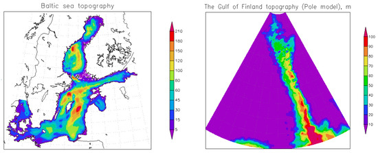
Figure 1.
Bottom topography of the Baltic Sea (left) and the Gulf of Finland.
7. Results of Numerical Experiments for Assessment of Marine Pollution
The numerical experiment consists of two steps. At the first step a monthly mean velocity field in the Baltic Sea is computed starting from initial temperature and salinity fields (provided by SOI data) and zero velocity. The numerical experiment was carried out for the period from 1 January 2007 to 31 December 2008. The model time step was equal to 5 min, the number of nodes in the Baltic Sea was 188,435 at each -level. We took the following coefficients and parameterization for the calculations. In the boundary conditions at the sea surface we have cm/s, and the coefficients of large-scale horizontal turbulent diffusion parameterization (in operator ) were taken equal to cm2/s. The coefficients of the fourth-order lateral viscosity were taken as cm4/s. The coefficients of vertical viscosity and diffusion were taken according to the Pacanowsky–Philander parameterization [41]. The coefficients were bounded by the minimal and maximal values. The viscosity coefficient varied from 1 to 50 cm2/s, the diffusion coefficient for the temperature varied from its background value 0.005 to 0.5 cm2/s, the coefficient for the salinity varied from the background value 0.001 to 0.1 cm2/s. In order to avoid “thinning” of the vertical temperature profiles in the near-surface layer, we took the diffusion coefficients for the temperature, salinity and viscosity equal to 5 cm2/s in the upper 2.5-m layer. At the second step the adjoint problem for sensitivity function with a prescribed monthly mean velocity field is solved. As a protected area we choose the Tallinn–Helsinki region (Figure 2). Based on the results the following features can be noted.
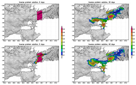
Figure 2.
Influence function and “inverse” velocity field: 0, 5, 30, and 40 days.
The use of high-resolution regional sea models has become important in recent times, first of all due to the development of operational oceanography, coastal ecological investigations, and management systems. In our study we used the sea numerical model with improved resolution in the eastern part of the Gulf of Finland. It made possible to describe eddy variability and more accurately represent the sea currents responsible for the ecological contamination of this area.
Figure 2 shows an initial stage of the sensitivity function variation, back in time, with corresponding velocities. One can see that marine circulation contains vigorous mesoscale eddies at spatial scales from roughly 5 km. Figure 2 shows the structure of the sensitivity function at different time moments. It describes a corresponding impact of each environmental point of the Baltic Sea on the variation of the considered functional Equation (16). Maximums of the sensitivity function represent the most dangerous subregions of the Baltic Sea for the contamination of the Tallinn–Helsinki protected area by passive impurity.
There are four subdomains of the highest one-month impact of contamination of the Tallinn–Helsinki area. Two of them are the vicinities of Tallinn and Helsinki themselves, the third one is situated between the northern coast of Hiiumaa and western open Gulf of Finland waters, and the fourth is between Hiiumaa and the northern Estonian coast.
We also give the results of calculating the sensitivity function for the case when the protected area is the entire Gulf of Finland. The calculation of the adjoint problem was carried out by A.V. Gusev (INM RAS) for a period of more than 3 months, the field of currents averaged over 3 months was used. Figure 3, Figure 4 and Figure 5 show the results of calculating the sensitivity function. It can be seen that in process of time the influence of the main area of the Baltic Sea on the pollution of the Gulf of Finland is increasing. The structure of the sensitivity function corresponds qualitatively to the one previously considered for the protected Tallinn–Helsinki area.
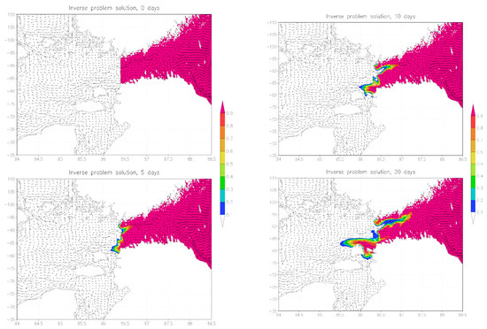
Figure 3.
Influence function and “inverse” velocity field: 0, 5, 10, and 20 days. Protected area: the Gulf of Finland.
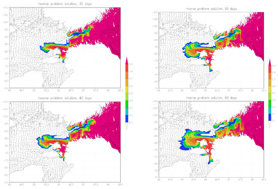
Figure 4.
Influence function and “inverse” velocity field: 30, 40, 50, and 60 days. Protected area: the Gulf of Finland.
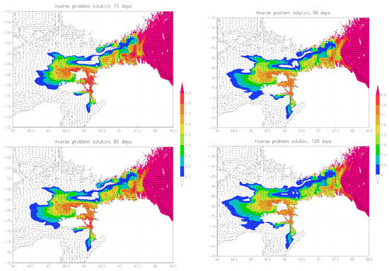
Figure 5.
Influence function and “inverse” velocity field: 70, 80, 90, and 100 days. Protected area: the Gulf of Finland.
Practical implementation of the results of the sensitivity function calculations enables development of solutions to better integrate the results of the growing body of research focused on the maritime traffic risk modeling [38] and the maritime accidents related to the ecological risk assessment [35]. Multiplication of the sensitivity function by the function describing probability of maritime traffic accidents related to marine environment pollution allows construction of a “risk map” with respect to potential pollution of the Tallinn–Helsinki protected area. In principle, integration of the sensitivity function and the results of maritime traffic risk modeling and the ecological risk assessment may be used as a scientific basis for development of proper methods and decision support tools based on multidisciplinary risk analysis to guide the authorities in decreasing risk in a cost-effective way, in particular, the environmental risk associated with ship routing.
8. Numerical Calculation of the Optimal Ship Route
This section is devoted to the results of calculating the optimal ship routes under the conditions of a stationary threat and a dynamic threat with a given trajectory. A series of numerical experiments was carried out taking into account the stationary threat when the ship passes through fixed zones (the intersection of which is characterized by a certain danger and possible damage), and taking into account the dynamic threat at the possible intersection of the ship’s route with the trajectory of another object.
The first cycle of experiments is aimed at solving the problem of minimizing the risk of marine accidents with a probable danger on the way of the ship. In the model area 150 km × 150 km, the coordinates and characteristics of the stationary threat, and the probability density of the incident with the ship were set. It was assumed that the original route of the ship is a straight line, the shortest distance between two points. Two cases of a possible emergence of a critical risk situation were calculated. Figure 6 and Figure 7 and Table 1 and Table 2 contain some results of the experiment described above. The red straight line denotes the initial (planned) trajectory of the vessel, convex black - the optimal route of the ship.
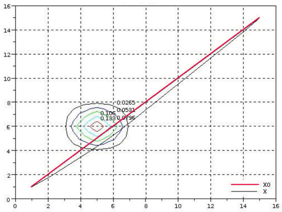
Figure 6.
Optimal ship route in the conditions of a stationary threat, , km.
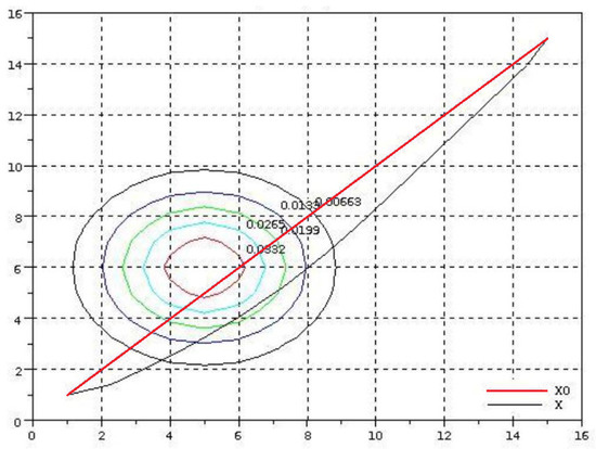
Figure 7.
Optimal ship route in the conditions of a stationary threat, , km.

Table 1.
The results of calculations for and km. Zero iteration represents the value of the functionals before the algorithm starts.

Table 2.
Results of calculations for the first cycle of experiments.
The second cycle of experiments is devoted to solving the problem of risk minimization in the conditions of a dynamic threat with a given trajectory of motion. In the model area 150 km × 150 km, the coordinates and characteristics of the dynamic threat, the trajectory of such a threat and the probability distribution of the critical situation at each point of the threat route were specified. It was assumed that the original route of the ship was a straight line, and the probable threat can be specified by the normal probability distribution. Two different situations are also presented. In the experiments, the specified design parameters gradually increased from minimal , km to more significant , km. Table 3 and Table 4 present the results of calculations for these two cases. Figure 8 shows the ship route (blue is the original, punctured blue is optimal) and the dynamic threat trajectory (red) for , km.

Table 3.
The results of calculations in the case of a dynamic threat with and km. Zero iteration represents the value of the functionals before the algorithm starts.

Table 4.
Results of calculations for the second cycle of experiments.
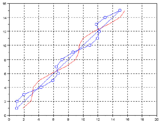
Figure 8.
Optimal ship route in the conditions of a dynamic threat, , km.
The third cycle of experiments is aimed at solving the problem of minimizing the risk in conditions of passage by a ship of a probable moving source of danger in the Baltic Sea. As a dynamic threat, the movement of another ship is considered here. From open sources, information was received on the shipping routes in the region (see www.marinetraffic.com). We calculated the case of a critical situation at the intersection of trade and industrial routes between Estonia and Finland and from Saint Petersburg. The calculations were carried out on a 5-km grid with a resolution of in latitude and in longitude, at zero wind. As a result, optimal routes were obtained taking into account the danger on the way of the ship. The results are shown in Figure 9. In all cases, to solve the optimization problem, it took 3–4 iterations of the iterative method described in Section 5.
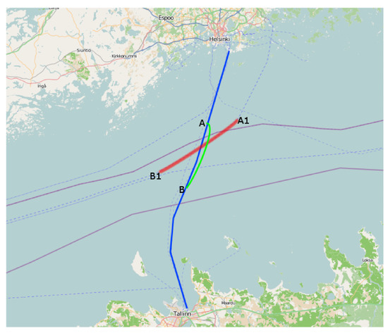
Figure 9.
Optimal ship route in the conditions of a dynamic threat. The blue color is the original route, green is the optimal one, and red is the trajectory of danger.
9. Conclusions
In this paper, we propose methods and technology for solving a wide range of problems in the dynamics of sea currents and assessing their “impact” on the objects of the marine environment using adjoint equations. The developed methods can be used for monitoring and forecasting the sea currents, for solving the problems of minimizing risks, and for analyzing marine disasters associated with the choice of the optimal ship route, assessing the pollution of coastal zones, etc. The technology includes a numerical model of marine circulation with improved resolution of coastal zones, a method for solving the inverse problem of contamination of the sea with a passive impurity, and a variational algorithm for constructing the optimal trajectory of the ship. Numerical experiments show the effectiveness of the developed methods for assessing marine pollution and calculating the optimal ship route under conditions of a stationary or dynamic threat (including the threat of a collision with another ship). When developing and testing the algorithms and programs in this article, the Baltic Sea was chosen as the marine area for certainty. However, the theoretical results and the computational algorithms under consideration can be extended to other areas.
Acknowledgments
This work was carried out within Russian Science Foundation project 14-11-00609 (studies in Section 4), project 15-05-00557 of the Russian Foundation for Basic Research, and the BONUS project “Strategic and operational risk management for wintertime maritime transportation system (BONUS STORMWINDS)”. The project was supported by BONUS (Art 185), funded jointly by the EU and the national funding institutions the Academy of Finland (Finland), the Estonian Research Council (Estonia), and the Research Council for Environment Agricultural Sciences and Spatial Planning (FORMAS) (Sweden).
Author Contributions
V.Z., V.A. and V.S. presented the theory, A.Z. performed the numerical experiments, R.A., F.G. and P.K. analysed the experiments.
Conflicts of Interest
The authors declare no conflict of interest. The founding sponsors had no role in the design of the study; in the collection, analyses, or interpretation of data; in the writing of the manuscript, and in the decision to publish the results.
References
- Druzhinin, O.A.; Ostrovsky, L.A.; Zilitinkevich, S.S. The study of the effect of small-scale turbulence on internal gravity waves propagation in a pycnocline. Nonlinear Processes Geophys. 2013, 20, 977–986. [Google Scholar] [CrossRef]
- Sarkisyan, A.; Sündermann, J. Modelling Ocean Climate Variability; Springer: Heidelberg, Germany, 2009. [Google Scholar]
- Thomas, L.N.; Tandon, A.; Mahadevan, A. Submesoscale processes and dynamics. In Ocean Modeling in an Eddying Regime; Hecht, M.W., Hasumi, H., Eds.; American Geophysical Union: Washington, DC, USA, 2008; pp. 17–38. [Google Scholar]
- Zalesny, V.B.; Gusev, A.V.; Agoshkov, V.I. Modeling Black Sea circulation with high resolution in the coastal zone. Izv. Atmos. Ocean. Phys. 2016, 52, 277–293. [Google Scholar] [CrossRef]
- Zalesny, V.; Gusev, A.; Chernobay, S.; Aps, R.; Tamsalu, R.; Kujala, P.; Rytkönen, J. The Baltic Sea circulation modeling and assessment of marine pollution. Russ. J. Numer. Anal. Math. Model. 2014, 29, 129–138. [Google Scholar] [CrossRef]
- Zalesny, V.B.; Gusev, A.V.; Lukyanova, A.N.; Fomin, V.V. Numerical modelling of sea currents and tidal waves. Russ. J. Numer. Anal. Math. Model. 2016, 31, 115–125. [Google Scholar] [CrossRef]
- Kordzadze, A.A.; Demetrashvili, D.I. Operative forecast of hydrophysical fields in the Georgian Black Sea coastal zone within the ECOOP. Ocean Sci. 2011, 7, 793–803. [Google Scholar] [CrossRef]
- Kordzadze, A.A.; Demetrashvili, D.I. Short-range forecast of hydrophysical fields in the eastern part of the Black Sea. Izv. Atmos. Ocean. Phys. 2013, 49, 674–685. [Google Scholar] [CrossRef]
- Kordzadze, A.A.; Demetrashvili, D.I.; Surmava, A.A. Numerical modeling of hydrophysical fields of the Black Sea under the conditions of alternation of atmospheric circulation processes. Izv. Atmos. Ocean. Phys. 2008, 44, 213–224. [Google Scholar] [CrossRef]
- Kubryakov, A.; Grigoriev, A.; Kordzadze, A.; Korotaev, G.; Stefanescu, S.; Trukhchev, D.; Fomin, V. Nowcasting/forecasting subsystem of the circulation in the Black Sea nearshore regions. In European Operational Oceanography: Present and Future, Proceedings of the 4th EuroGOOS Conference, Brest, France, 6–9 June 2005; EuroGOOS Office: Norrköping, Sweden, 2006; pp. 605–610. [Google Scholar]
- Agoshkov, V.I.; Assovskii, M.V.; Zalesny, V.B.; Zakharova, N.B.; Parmuzin, E.I.; Shutyaev, V.P. Variational assimilation of observation data in the mathematical model of the Black Sea taking into account the tides generating forces. Russ. J. Numer. Anal. Math. Model. 2015, 30, 129–142. [Google Scholar] [CrossRef]
- Agoshkov, V.I.; Parmuzin, E.I.; Zalesny, V.B.; Shutyaev, V.P.; Zakharova, N.B.; Gusev, A.V. Variational assimilation of observation data in the mathematical model of the Baltic Sea dynamics. Russ. J. Numer. Anal. Math. Model. 2015, 30, 203–212. [Google Scholar] [CrossRef]
- Aseev, N.A.; Agoshkov, V.I.; Zalesny, V.B.; Aps, R.; Kujala, P.; Rytkönen, J. The problem of control of oil pollution risk in the Baltic Sea. Russ. J. Numer. Anal. Math. Model. 2014, 29, 93–106. [Google Scholar] [CrossRef]
- Bezhenar, R.; Jung, K.-T.; Maderich, V.; Kim, K.-O. 3D numerical model of ecohydrodynamics for shallow waters. J. Coast. Res. 2016, 75, 820–824. [Google Scholar] [CrossRef]
- Leppäranta, M.; Myrberg, K. Physical Oceanography of the Baltic Sea; Springer-Praxis: Heidelberg, Germany, 2009. [Google Scholar]
- Zalesny, V.B.; Diansky, N.A.; Fomin, V.V.; Moshonkin, S.N.; Demyshev, S.G. Numerical model of the circulation of the Black Sea and the Sea of Azov. Russ. J. Numer. Anal. Math. Model. 2012, 27, 95–111. [Google Scholar] [CrossRef]
- Zalesny, V.B.; Gusev, A.V.; Ivchenko, V.O.; Tamsalu, R.; Aps, R. Numerical model of the Baltic Sea circulation. Russ. J. Numer. Anal. Math. Model. 2013, 28, 85–100. [Google Scholar] [CrossRef]
- Zalesny, V.B.; Gusev, A.V.; Moshonkin, S.N. Numerical model of the hydrodynamics of the Black Sea and the Sea of Azov with variational initialization of temperature and salinity. Izv. Atmos. Ocean. Phys. 2013, 49, 642–658. [Google Scholar] [CrossRef]
- Zalesny, V.B.; Marchuk, G.I.; Agoshkov, V.I.; Bagno, A.V.; Gusev, A.V.; Diansky, N.A.; Moshonkin, S.N.; Tamsalu, R.; Volodin, E.M. Numerical simulation of large-scale ocean circulation based on the multicomponent splitting method. Russ. J. Numer. Anal. Math. Model. 2010, 25, 581–609. [Google Scholar] [CrossRef]
- Zalesny, V.B.; Tamsalu, R. High-resolution modeling of a marine ecosystem using the FRESCO hydroecological model. Izv. Atmos. Ocean. Phys. 2009, 45, 102–115. [Google Scholar] [CrossRef]
- Zalesny, V.B.; Tamsalu, R.; Mannik, A. Multidisciplinary numerical model of a coastal water ecosystem. Russ. J. Numer. Anal. Math. Model. 2008, 23, 207–222. [Google Scholar] [CrossRef]
- Blayo, E.; Debreu, L. Nesting ocean models. In Ocean Weather Forecasting: An Integrated View of Oceanography; Chassignet, E.P., Verron, J., Eds.; Springer: Heidelberg, Germany, 2006; pp. 127–146. [Google Scholar]
- Piggott, M.D.; Pain, C.C.; Gorman, G.J.; Marshall, D.P.; Killworth, P.D. Unstructured adaptive meshes for ocean modeling. In Ocean Modeling in an Eddying Regime; Hecht, M.W., Hasumi, H., Eds.; American Geophysical Union: Washington, DC, USA, 2008; pp. 383–408. [Google Scholar]
- Deleersnijder, E.; Lermusiaux, P.F.J. Multi-scale modeling: nested-grid and unstructured-mesh approaches. Ocean Dyn. 2008, 58, 335–498. [Google Scholar] [CrossRef]
- Griffies, S.M.; Boening, C.; Bryan, F.O.; Chassignet, E.P.; Gerdes, R.; Hasumi, H.; Hirst, A.; Treguier, A.-M.; Webb, D. Developments in ocean climate modelling. Ocean Model. 2000, 2, 123–192. [Google Scholar] [CrossRef]
- Ilicak, M.; Adcroft, A.J.; Legg, S. A framework for parameterization of heterogeneous ocean convection. Ocean Model. 2014, 82, 1–14. [Google Scholar] [CrossRef]
- Porta Mana, P.G.L.; Zanna, L. Toward a stochastic parameterization of ocean mesoscale eddies. Ocean Model. 2014, 79, 1–20. [Google Scholar] [CrossRef]
- Marchuk, G.I. Splitting and alternative direction methods. In Handbook of Numerical Analysis, V.1; Ciarlet, P.G., Lions, J.L., Eds.; North-Holland: Amsterdam, The Netherlands, 1990; pp. 197–462. [Google Scholar]
- Marchuk, G.I. Adjoint Equations and Analysis of Complex Systems; Kluwer: Dordrecht, The Netherlands, 1995. [Google Scholar]
- Agoshkov, V.I. Adjoint equations and perturbation algorithms in the problem of optimal trajectories. In Computational Mathematics and Mathematical Modelling, Proceedings of the International Conference; Dymnikov, V.P., Ed.; INM RAS: Moscow, Russia, 2000; Volume 1, pp. 36–53. [Google Scholar]
- Agoshkov, V.I. Methods of Optimal Control and Adjoint Equations in Problems of Mathematical Physics; INM RAS: Moscow, Russia, 2003. [Google Scholar]
- Agoshkov, V.I.; Aseev, N.A.; Zakharova, N.B.; Parmuzin, E.I.; Sheloput, T.O.; Shutyaev, V.P. Informational Computational System “RAS – Baltic Sea”; INM RAS: Moscow, Russia, 2016. [Google Scholar]
- Agoshkov, V.I.; Zayachkovskii, A.O. The study and solution algorithms for the problem of optimal ship routing based on the risk theory and remote danger sensing. Contemp. Prob. Earth Remote Sens. Outer Space 2012, 9, 9–17. [Google Scholar]
- Agoshkov, V.I.; Zayachkovskiy, A.O.; Aps, R.; Kujala, P.; Rytkönen, J. Risk theory based solution to the problem of optimal vessel route. Russ. J. Numer. Anal. Math. Model. 2014, 29, 69–78. [Google Scholar] [CrossRef]
- Aps, R.; Fetissov, M.; Herkül, K.; Kotta, J.; Leiger, R.; Mander, Ü.; Suursaar, Ü. Bayesian inference for predicting potential oil spill related ecological risk. In Safety and Security Engineering III; M. Guarascio, M., Brebbia, C.A., Garzia, F., Eds.; WIT Press: Southampton-Boston, UK, 2009; pp. 149–159. [Google Scholar]
- Dankel, D.J.; Aps, R.; Padda, G.; Röckmann, C.; van der Sluijs, J.P.; Wilson, D.C.; Degnbol, P. Advice under uncertainty in the marine system. ICES J. Mar. Sci. 2012, 69, 3–7. [Google Scholar] [CrossRef]
- Goerlandt, F.; Kujala, P. Traffic simulation based ship collision probability modeling. Reliab. Eng. Syst. Saf. 2011, 96, 91–107. [Google Scholar] [CrossRef]
- Kujala, P.; Hänninen, M.; Arola, T.; Ylitalo, J. Analysis of the marine traffic safety in the Gulf of Finland. Reliab. Eng. Syst. Saf. 2009, 94, 1349–1357. [Google Scholar] [CrossRef]
- Montewka, J.; Goerlandt, F.; Kujala, P. Determination of collision criteria and causation factors appropriate to a model for estimating the probability of maritime accidents. Ocean Engrg. 2012, 40, 50–61. [Google Scholar] [CrossRef]
- Muschick, E.; Müller, P.H. Eintscheidungspraxis; VEB Verlag Technik: Berlin, Germany, 1987. [Google Scholar]
- Pacanowsky, R.C.; Philander, G. Parameterization of vertical mixing in numerical models of the tropical ocean. J. Phys. Oceanogr. 1981, 11, 1442–1451. [Google Scholar] [CrossRef]
- Sonninen, S.; Nuutinen, M.; Rosqvist, T. Development Process of the Gulf of Finland Mandatory Ship Reporting System. Reflections on the Methods; VTT Publications 614: Espoo, Finland, 2006. [Google Scholar]
- Vishnyakov, Y.D.; Radaev, N.N. General Risk Theory; Publ. Center Akademia: Moscow, Russia, 2008. [Google Scholar]
- Vainberg, M.M. The Variational Method and the Method of Monotone Operators in the Theory of Nonlinear Equations; Nauka: Moscow, Russia, 1972. [Google Scholar]
- Marchuk, G.I.; Agoshkov, V.I.; Shutyaev, V.P. Adjoint Equations and Perturbation Algorithms in Nonlinear Problems; CRC Press Inc.: New York, NY, USA, 1996. [Google Scholar]
- Marchuk, G.I. Methods of Numerical Mathematics; Springer: Heidelberg, Germany, 1982. [Google Scholar]
© 2017 by the authors. Licensee MDPI, Basel, Switzerland. This article is an open access article distributed under the terms and conditions of the Creative Commons Attribution (CC BY) license (http://creativecommons.org/licenses/by/4.0/).