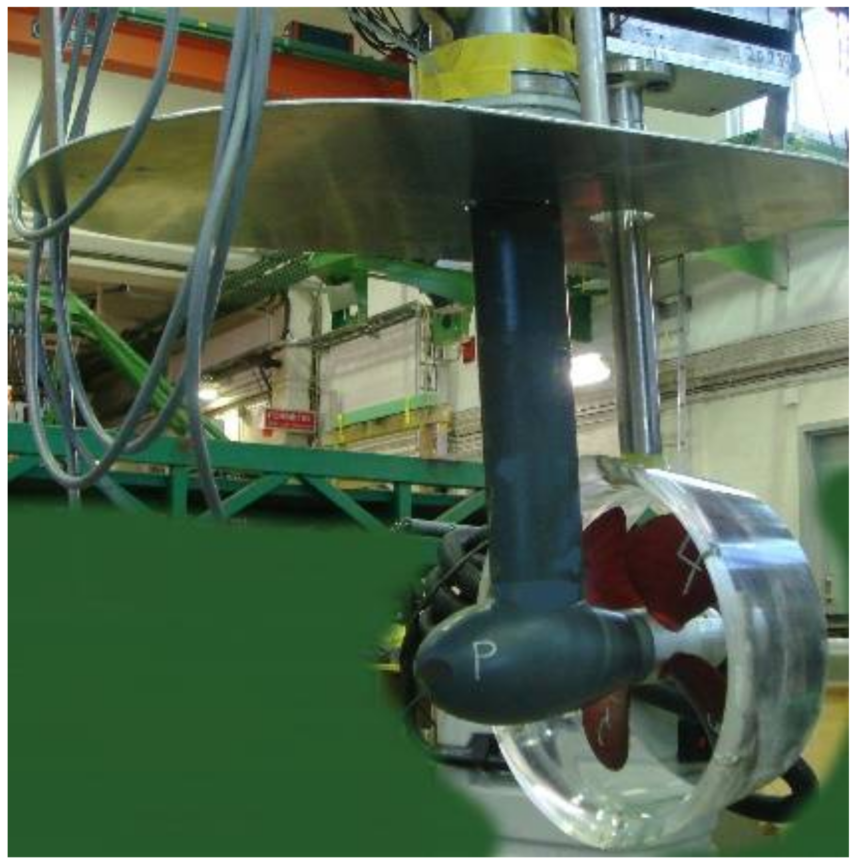
Figure 1.
General view of model test setup.
Figure 1.
General view of model test setup.
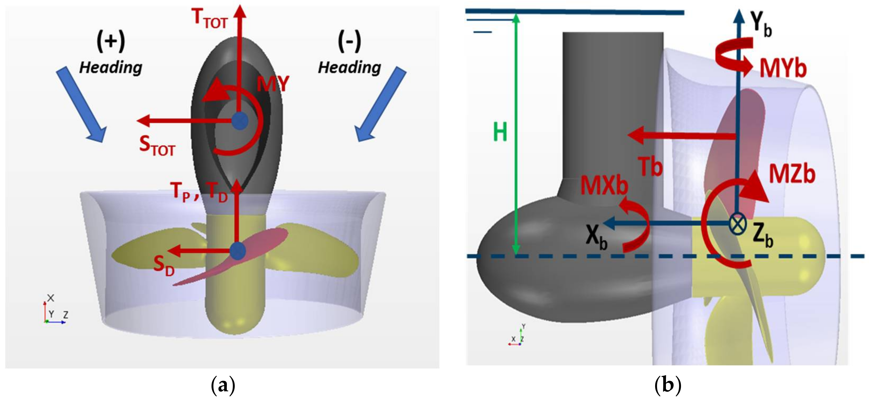
Figure 2.
Definitions of forces and moments and sign conventions: (a) propulsor loads; (b) blade loads.
Figure 2.
Definitions of forces and moments and sign conventions: (a) propulsor loads; (b) blade loads.
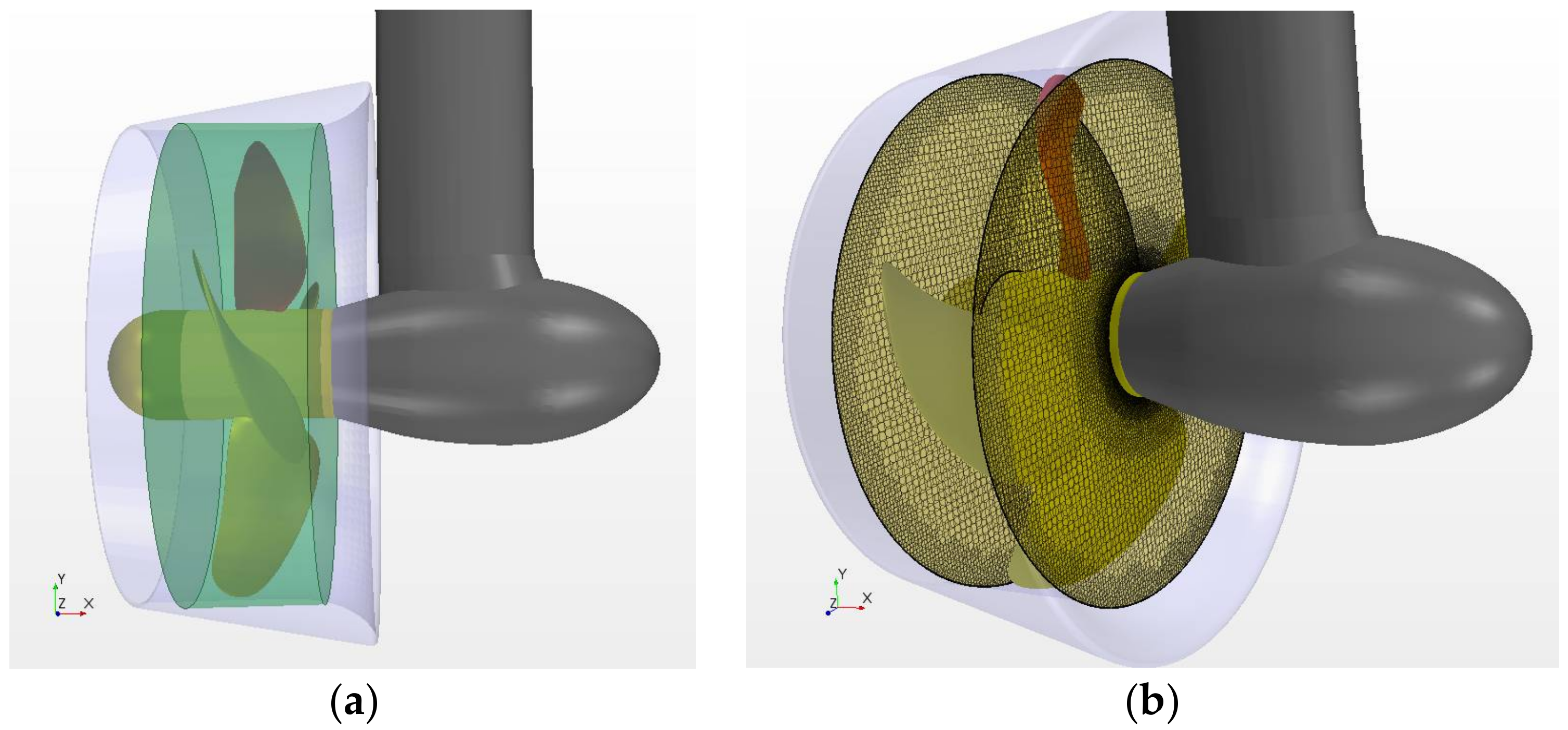
Figure 3.
Rotating propeller region and sliding mesh interfaces: (a) propeller region; (b) sliding interfaces.
Figure 3.
Rotating propeller region and sliding mesh interfaces: (a) propeller region; (b) sliding interfaces.
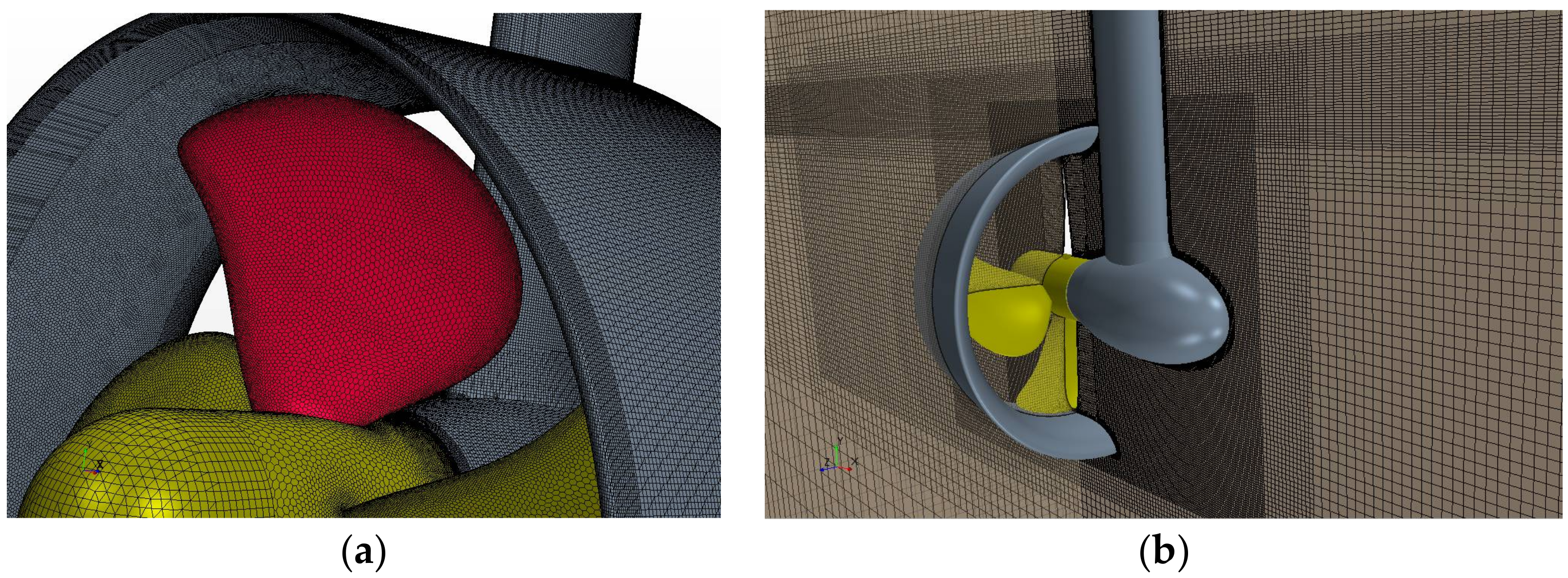
Figure 4.
Details of computation mesh: (a) surface mesh on propeller and duct; (b) volume mesh around propulsor and free surface.
Figure 4.
Details of computation mesh: (a) surface mesh on propeller and duct; (b) volume mesh around propulsor and free surface.
Figure 5.
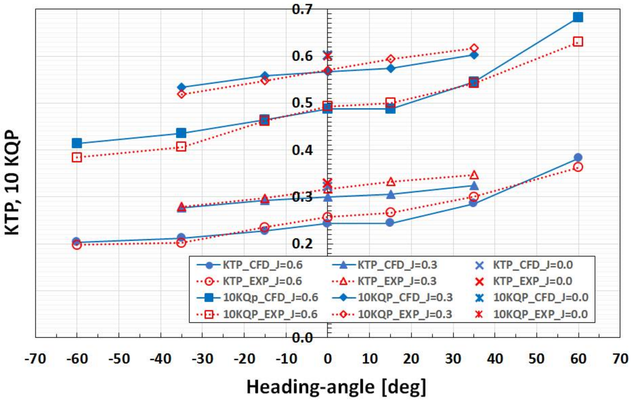
Measured (red) and computed (blue) propeller thrust, KTP, and propeller torque, KQP, at different heading angles and loading conditions.
Figure 5.
Measured (red) and computed (blue) propeller thrust, KTP, and propeller torque, KQP, at different heading angles and loading conditions.
Figure 6.
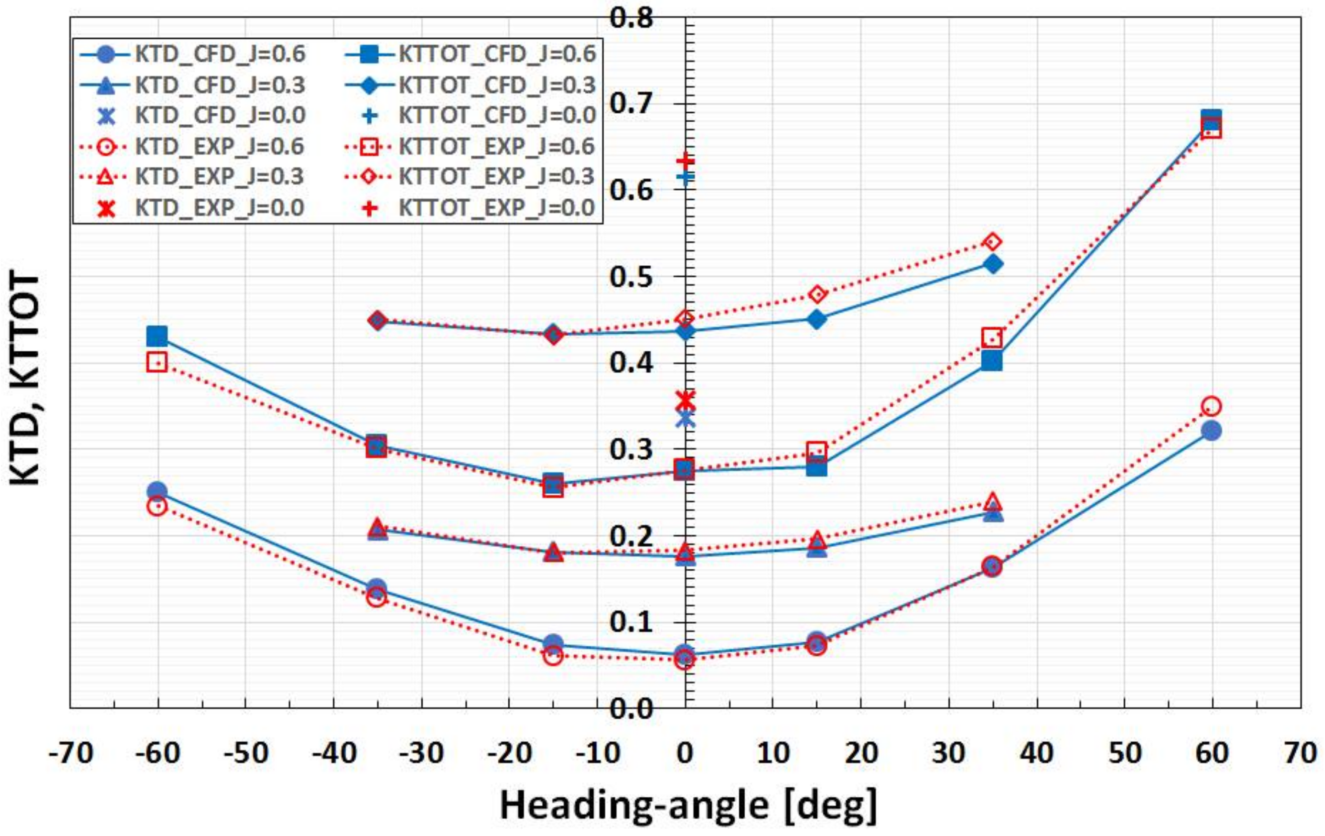
Measured (red) and computed (blue) duct thrust, KTD, and total unit thrust, KTTOT, at different heading angles and loading conditions.
Figure 6.
Measured (red) and computed (blue) duct thrust, KTD, and total unit thrust, KTTOT, at different heading angles and loading conditions.
Figure 7.
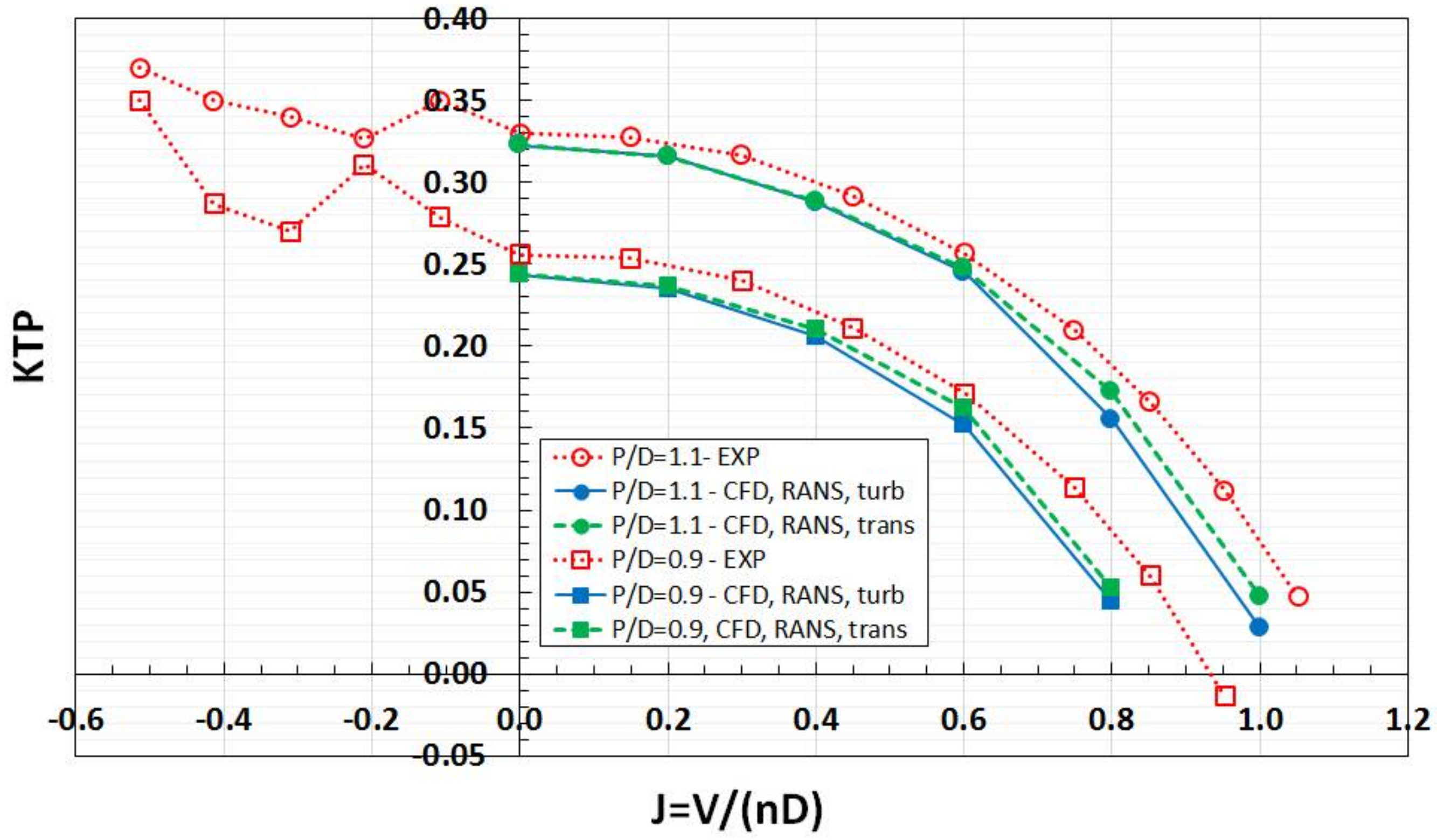
Measured (red) and computed (blue—fully turbulent model, green—transition model) propeller thrust, KTP, at the two propeller pitch settings, P/D, and different loading conditions.
Figure 7.
Measured (red) and computed (blue—fully turbulent model, green—transition model) propeller thrust, KTP, at the two propeller pitch settings, P/D, and different loading conditions.
Figure 8.
Measured (red) and computed (blue—fully turbulent model, green—transition model) propeller torque, KQP, at the two propeller pitch settings, P/D, and different loading conditions.
Figure 8.
Measured (red) and computed (blue—fully turbulent model, green—transition model) propeller torque, KQP, at the two propeller pitch settings, P/D, and different loading conditions.
Figure 9.
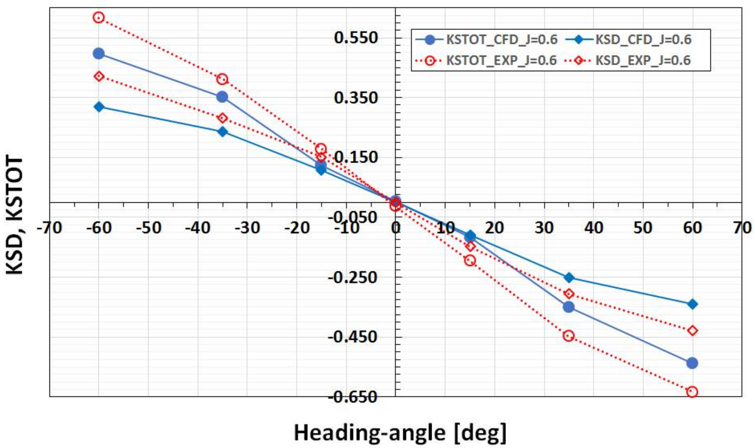
Measured (red) and computed (blue) duct side force, KSD, and total unit side force, KSTOT, at different heading angles and loading condition of J = 0.6.
Figure 9.
Measured (red) and computed (blue) duct side force, KSD, and total unit side force, KSTOT, at different heading angles and loading condition of J = 0.6.
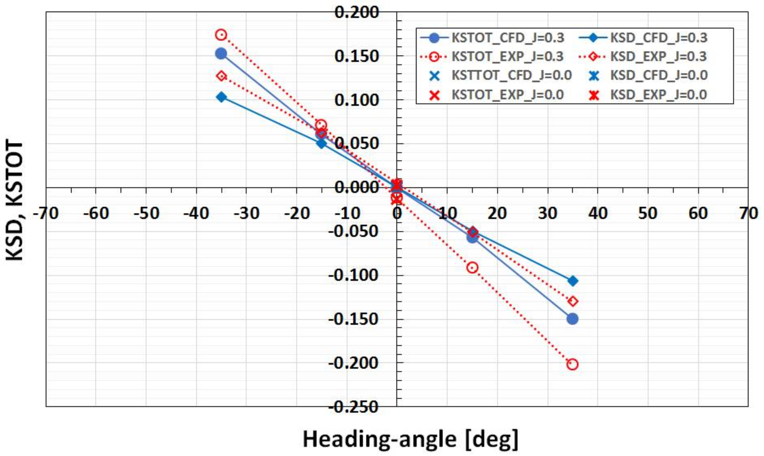
Figure 10.
Measured (red) and computed (blue) duct side force, KSD, and total unit side force, KSTOT, at different heading angles and loading conditions of J = 0.3 and J = 0.0.
Figure 10.
Measured (red) and computed (blue) duct side force, KSD, and total unit side force, KSTOT, at different heading angles and loading conditions of J = 0.3 and J = 0.0.
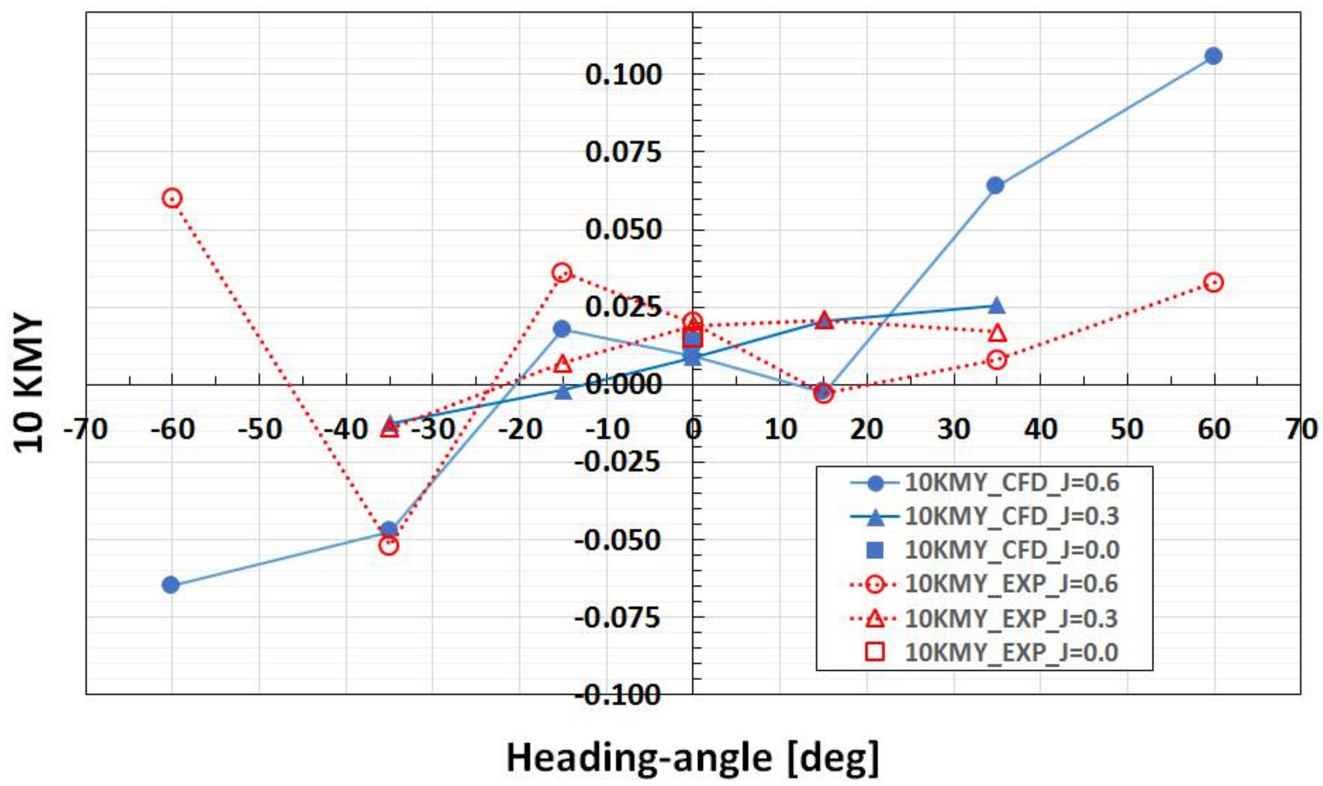
Figure 11.
Measured (red) and computed (blue) steering moment, KMY, excluding duct contribution, at different heading angles and loading conditions.
Figure 11.
Measured (red) and computed (blue) steering moment, KMY, excluding duct contribution, at different heading angles and loading conditions.
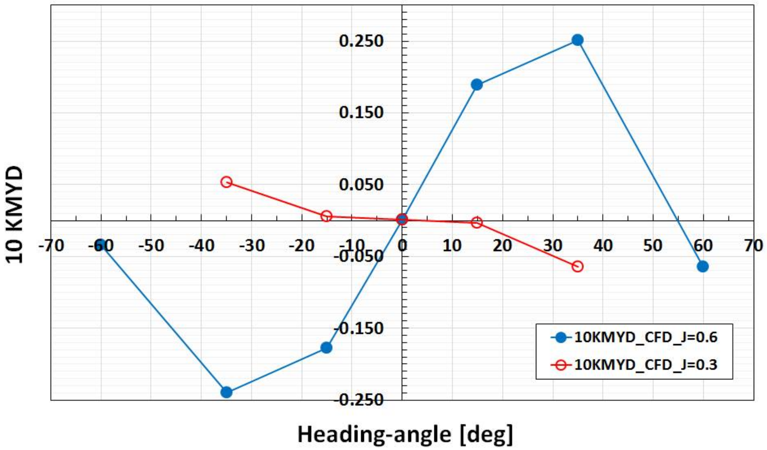
Figure 12.
Computed steering moment on the duct, KMYD, at different heading angles and loading conditions.
Figure 12.
Computed steering moment on the duct, KMYD, at different heading angles and loading conditions.
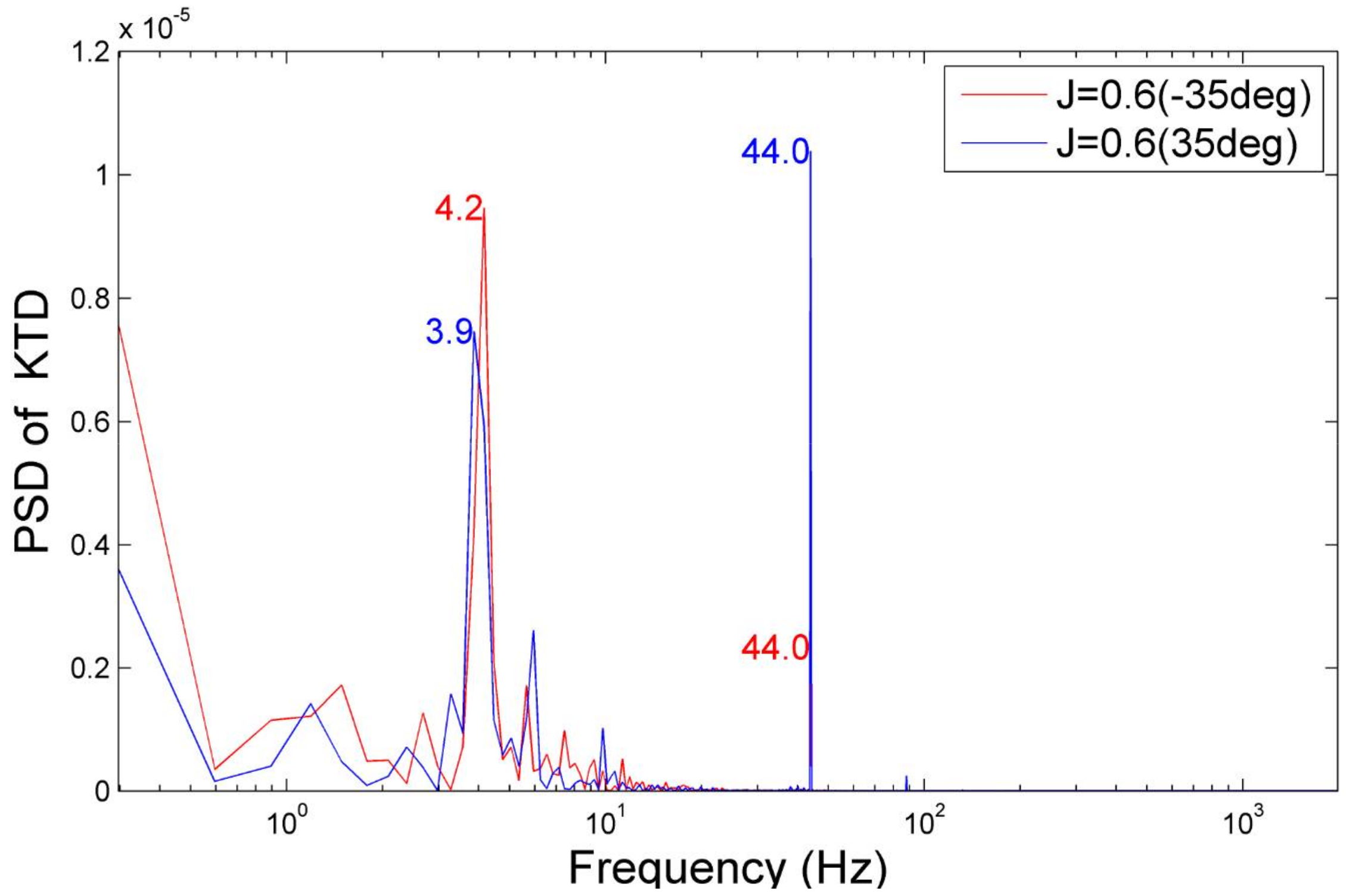
Figure 13.
Power spectral density of duct thrust, KTD, at J = 0.6, for the positive and negative heading angles of 35 degrees.
Figure 13.
Power spectral density of duct thrust, KTD, at J = 0.6, for the positive and negative heading angles of 35 degrees.
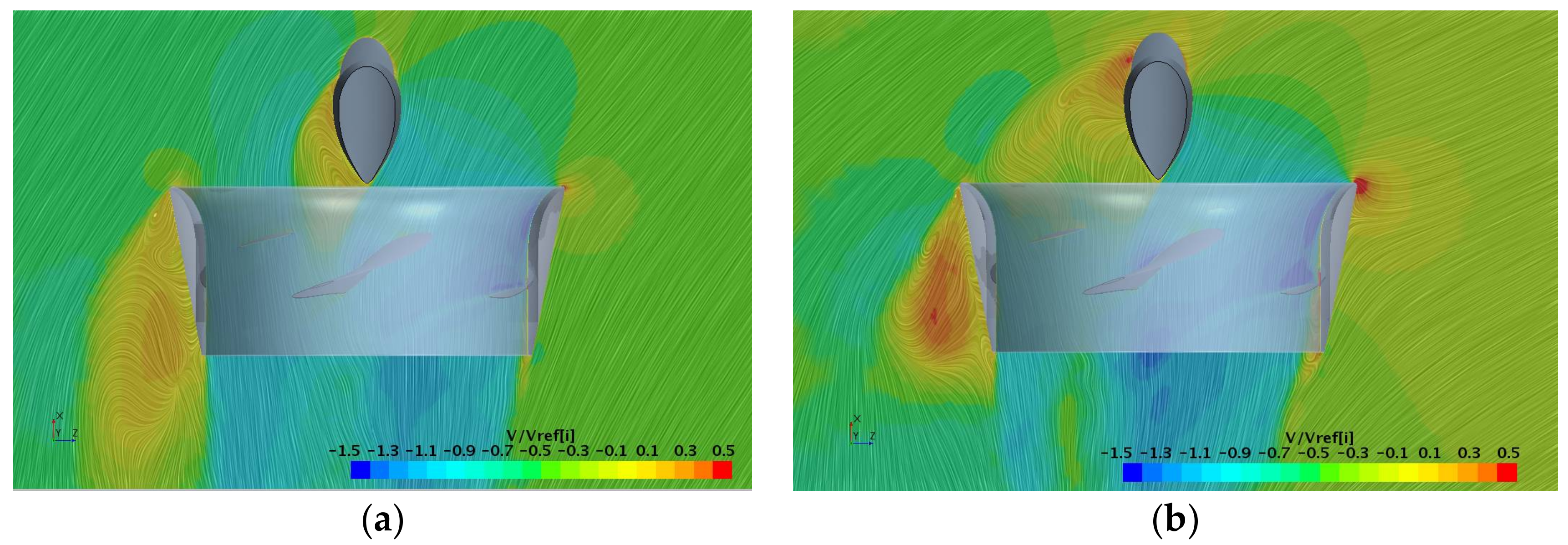
Figure 14.
Examples of flow pattern around propulsor at large heading angles, J = 0.6: (a) −35 degrees; (b) −60 degrees. View from top.
Figure 14.
Examples of flow pattern around propulsor at large heading angles, J = 0.6: (a) −35 degrees; (b) −60 degrees. View from top.
Figure 15.
Measured and computed time histories of blade loads at J = 0.6 for the heading angle +35°: (a) blade thrust, KTb; (b) blade bending moment, KMZb.
Figure 15.
Measured and computed time histories of blade loads at J = 0.6 for the heading angle +35°: (a) blade thrust, KTb; (b) blade bending moment, KMZb.
Figure 16.
Measured and computed time histories of blade loads at J = 0.6 for the heading angle −35°: (a) blade thrust, KTb; (b) blade bending moment, KMZb.
Figure 16.
Measured and computed time histories of blade loads at J = 0.6 for the heading angle −35°: (a) blade thrust, KTb; (b) blade bending moment, KMZb.
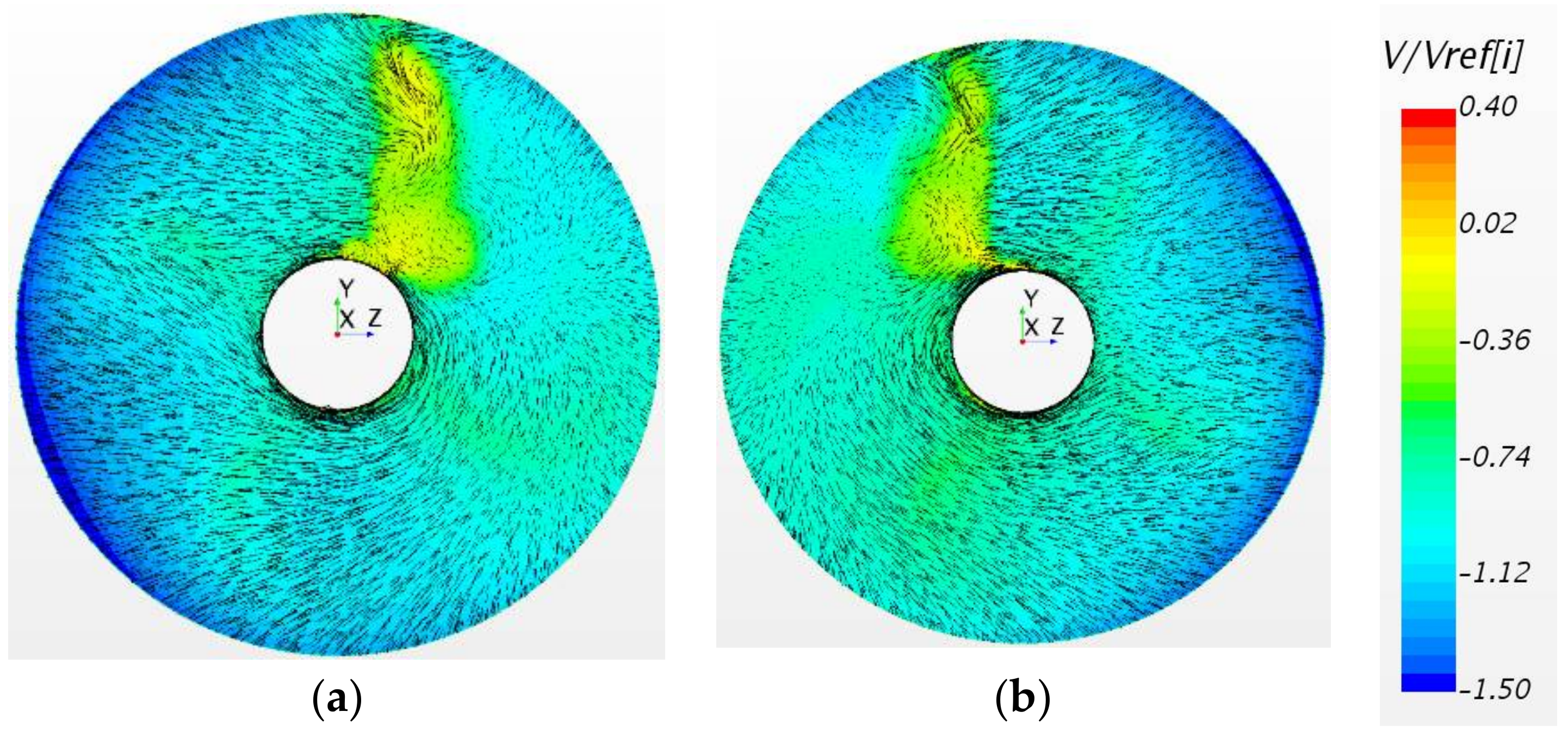
Figure 17.
Computed velocity fields on the control plane upstream of the propeller at J = 0.6 for positive and negative heading angles: (a) +35 degrees; (b) −35 degrees. View from downstream.
Figure 17.
Computed velocity fields on the control plane upstream of the propeller at J = 0.6 for positive and negative heading angles: (a) +35 degrees; (b) −35 degrees. View from downstream.
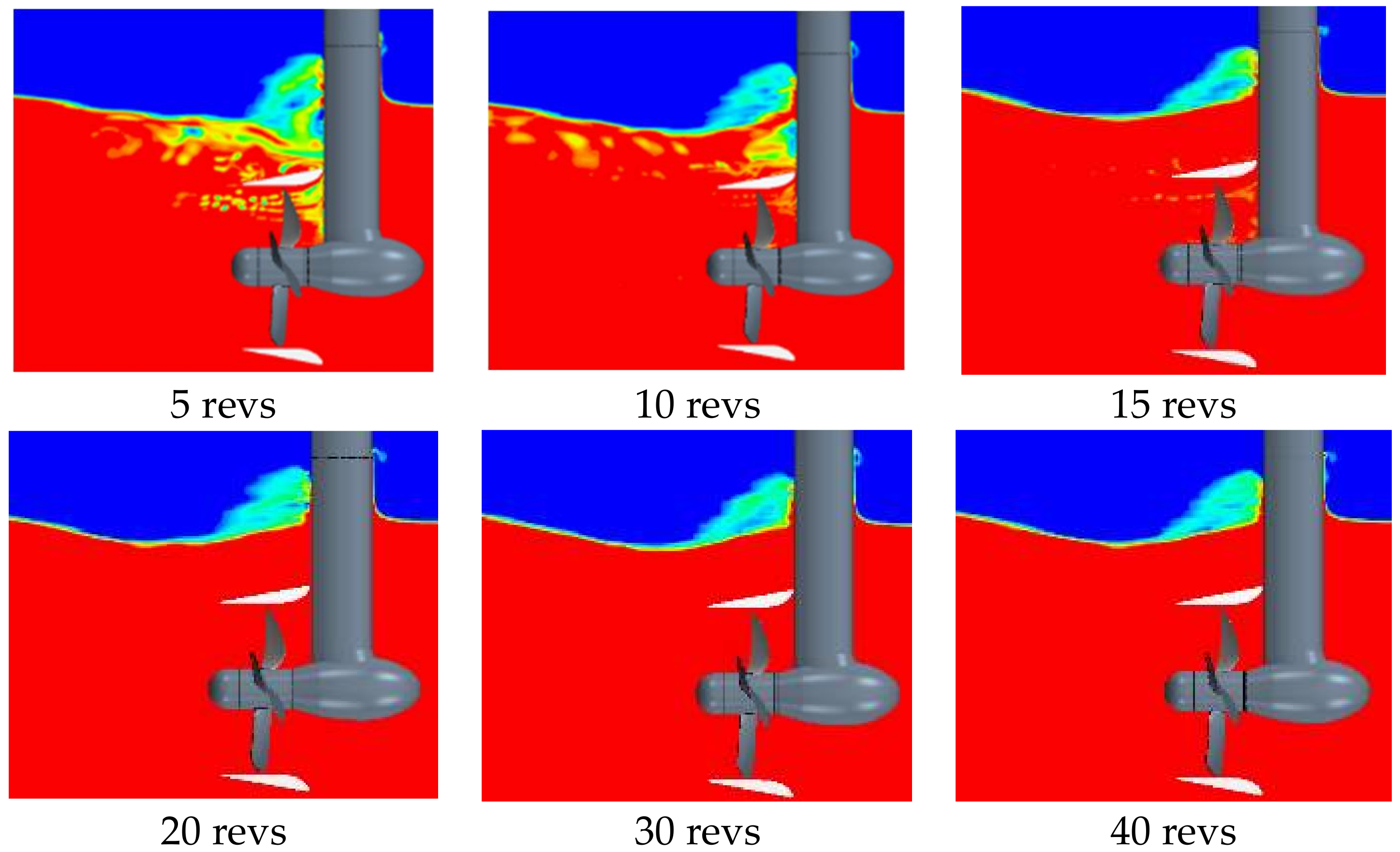
Figure 18.
Contours of volume fraction at different solution time instances for propulsor submergence H/Dp = 1.0, at J = 0.6.
Figure 18.
Contours of volume fraction at different solution time instances for propulsor submergence H/Dp = 1.0, at J = 0.6.
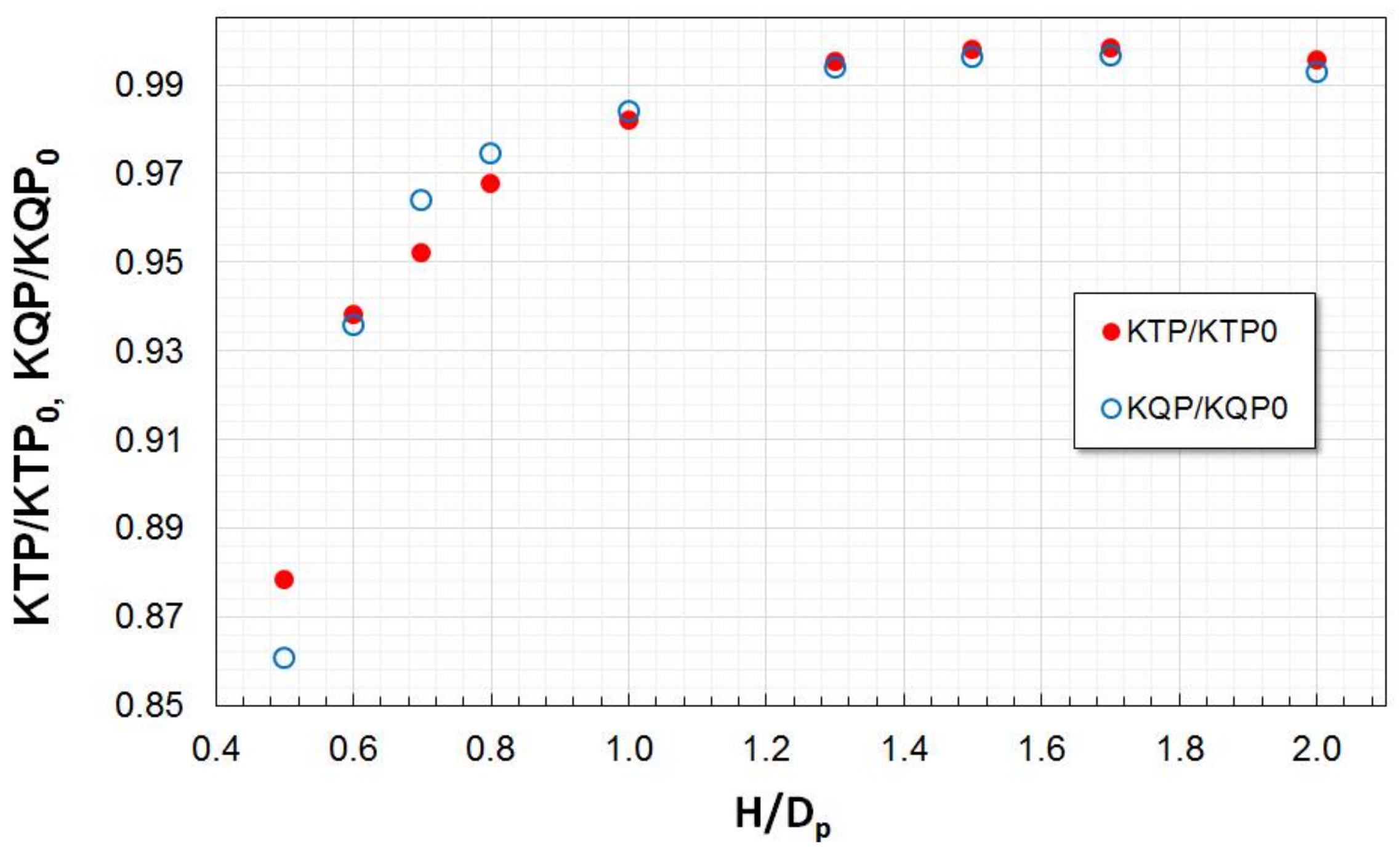
Figure 19.
Variations in propeller thrust, KTP, and propeller torque, KQP, with propulsor submergence, H/Dp, at J = 0.6. (KTP0, KQP0 refer to the corresponding values in unbounded flow).
Figure 19.
Variations in propeller thrust, KTP, and propeller torque, KQP, with propulsor submergence, H/Dp, at J = 0.6. (KTP0, KQP0 refer to the corresponding values in unbounded flow).
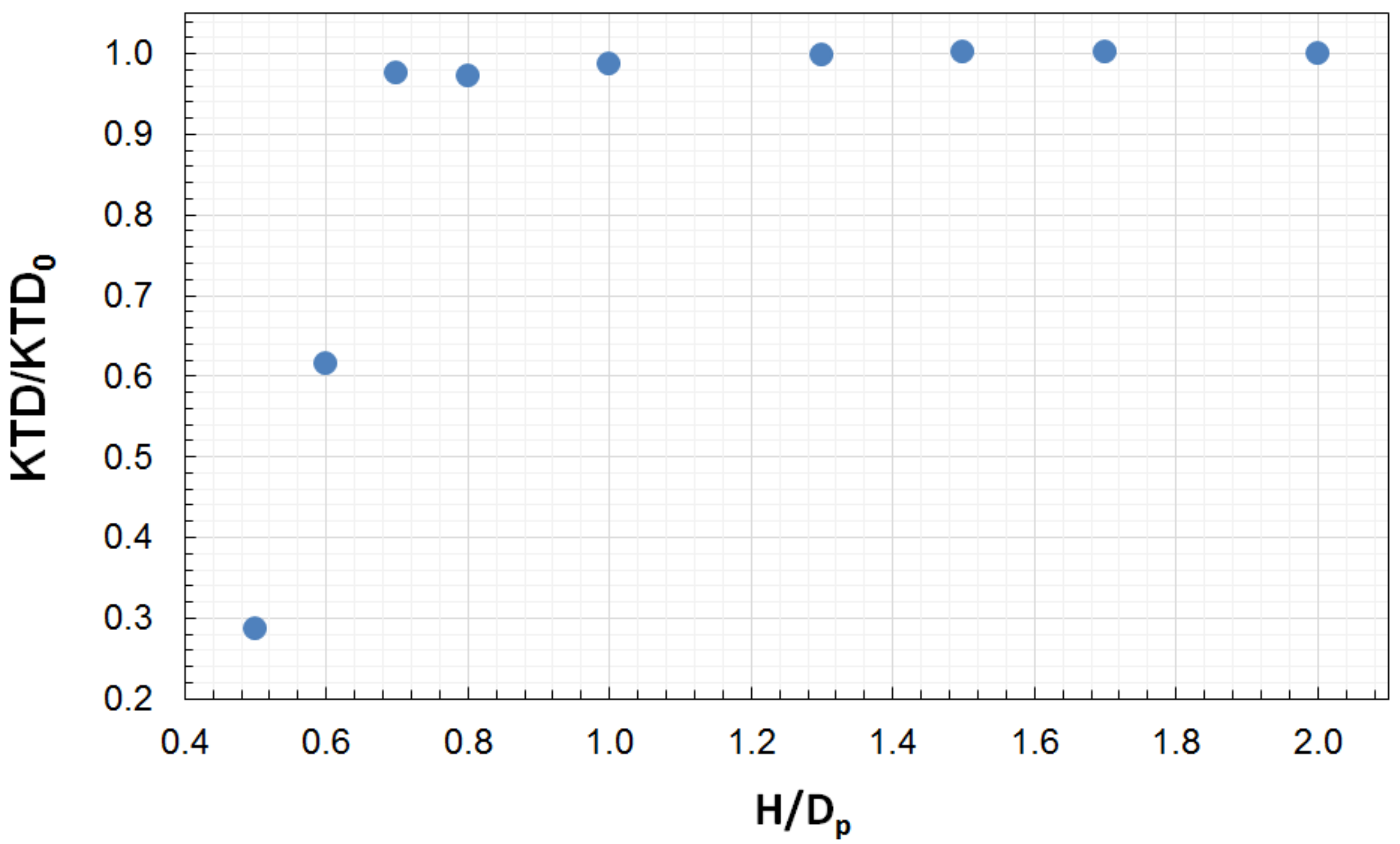
Figure 20.
Variations in duct thrust, KTD, with propulsor submergence, H/Dp, at J = 0.6. (KTD0 refers to the corresponding value in unbounded flow).
Figure 20.
Variations in duct thrust, KTD, with propulsor submergence, H/Dp, at J = 0.6. (KTD0 refers to the corresponding value in unbounded flow).
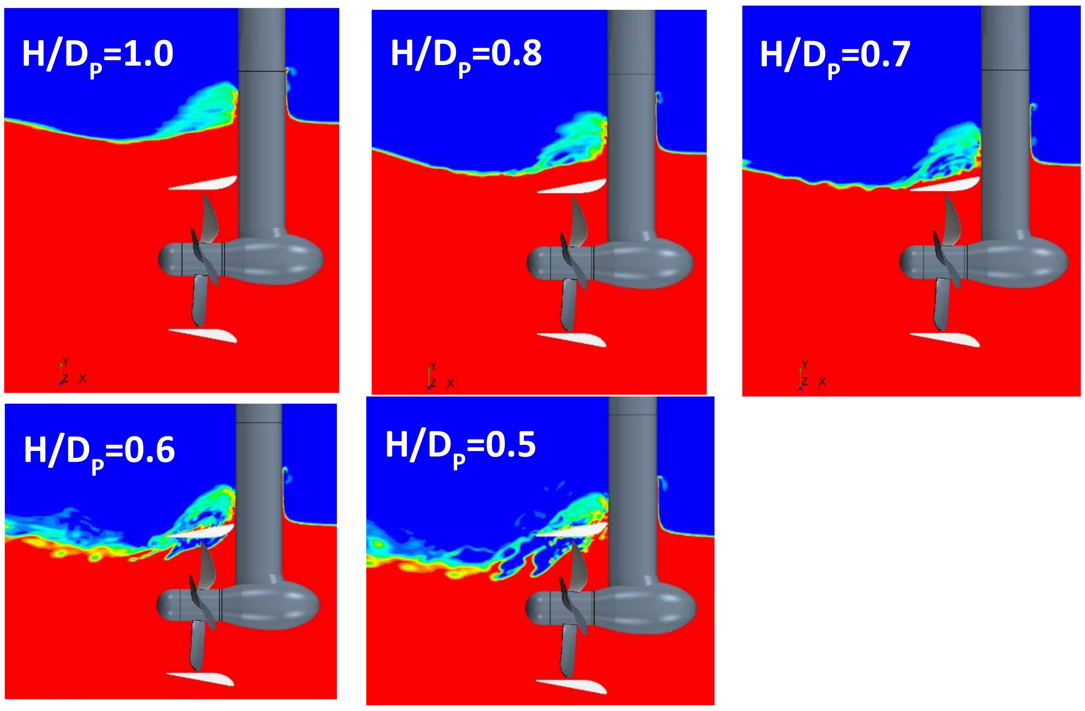
Figure 21.
Ventilation inception with decrease in propulsor submergence, H/Dp, at J = 0.6.
Figure 21.
Ventilation inception with decrease in propulsor submergence, H/Dp, at J = 0.6.
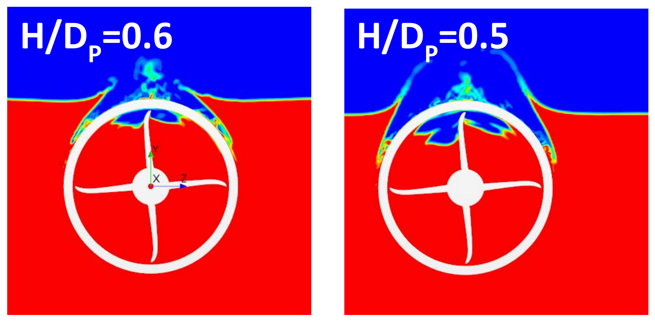
Figure 22.
Contours of volume fraction under fully ventilated conditions at the submergence values of H/Dp = 0.6 and 0.5, J = 0.6.
Figure 22.
Contours of volume fraction under fully ventilated conditions at the submergence values of H/Dp = 0.6 and 0.5, J = 0.6.
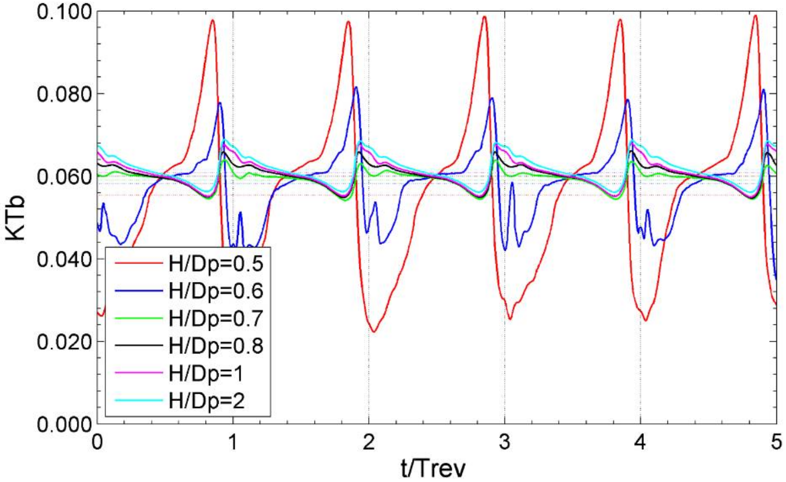
Figure 23.
Computed time histories of single blade thrust, KTb, for different magnitudes of submergence, H/Dp, at J = 0.6.
Figure 23.
Computed time histories of single blade thrust, KTb, for different magnitudes of submergence, H/Dp, at J = 0.6.
Figure 24.
Ventilation inception with decrease in propulsor submergence, H/Dp, at J = 0.2.
Figure 24.
Ventilation inception with decrease in propulsor submergence, H/Dp, at J = 0.2.
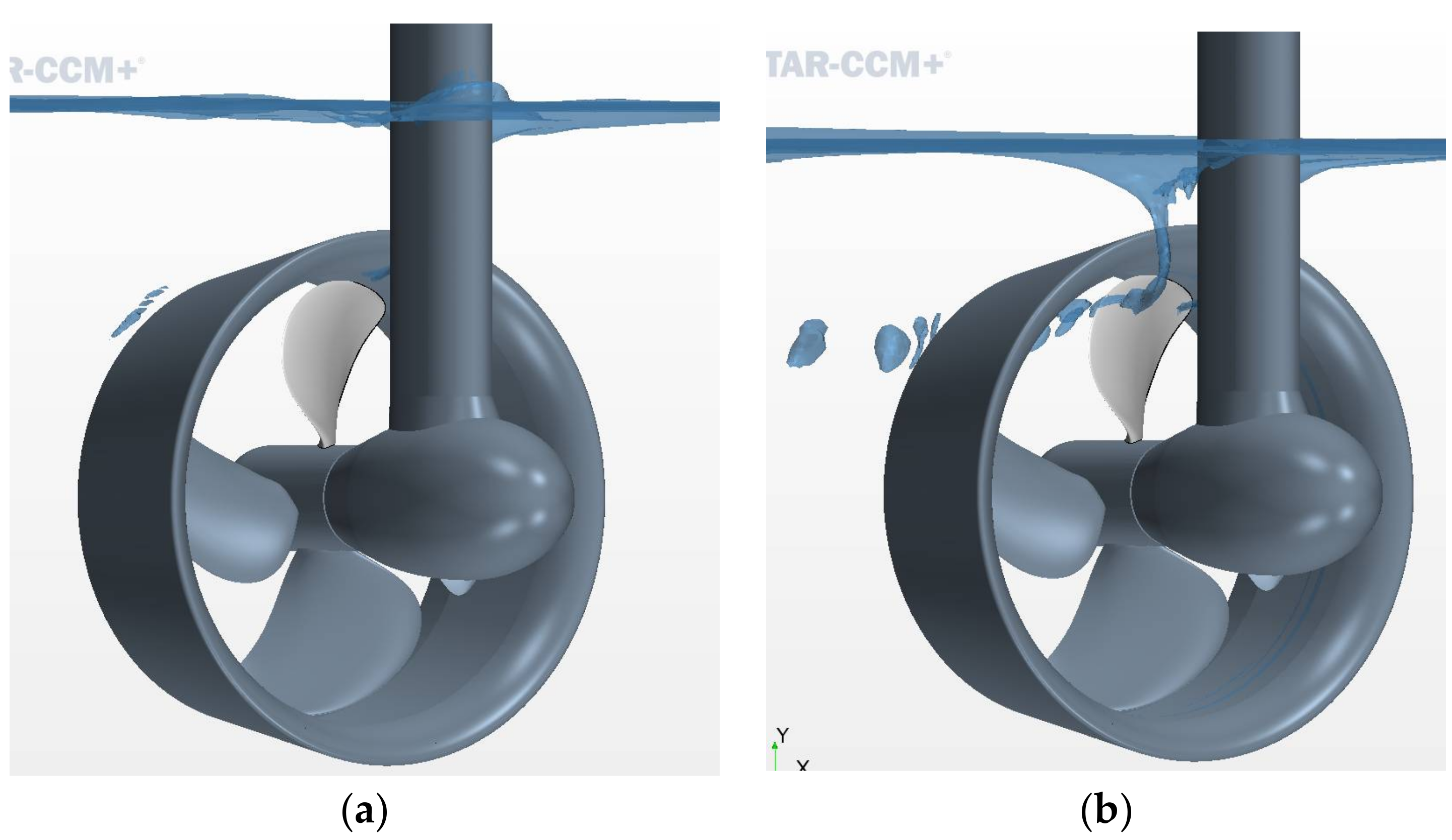
Figure 25.
Ventilation inception vortex at the conditions of heavy propulsor loading: (a) H/Dp = 0.9, at J = 0.2 (trawling); (b) H/Dp = 0.8, at J = 0.0 (bollard).
Figure 25.
Ventilation inception vortex at the conditions of heavy propulsor loading: (a) H/Dp = 0.9, at J = 0.2 (trawling); (b) H/Dp = 0.8, at J = 0.0 (bollard).
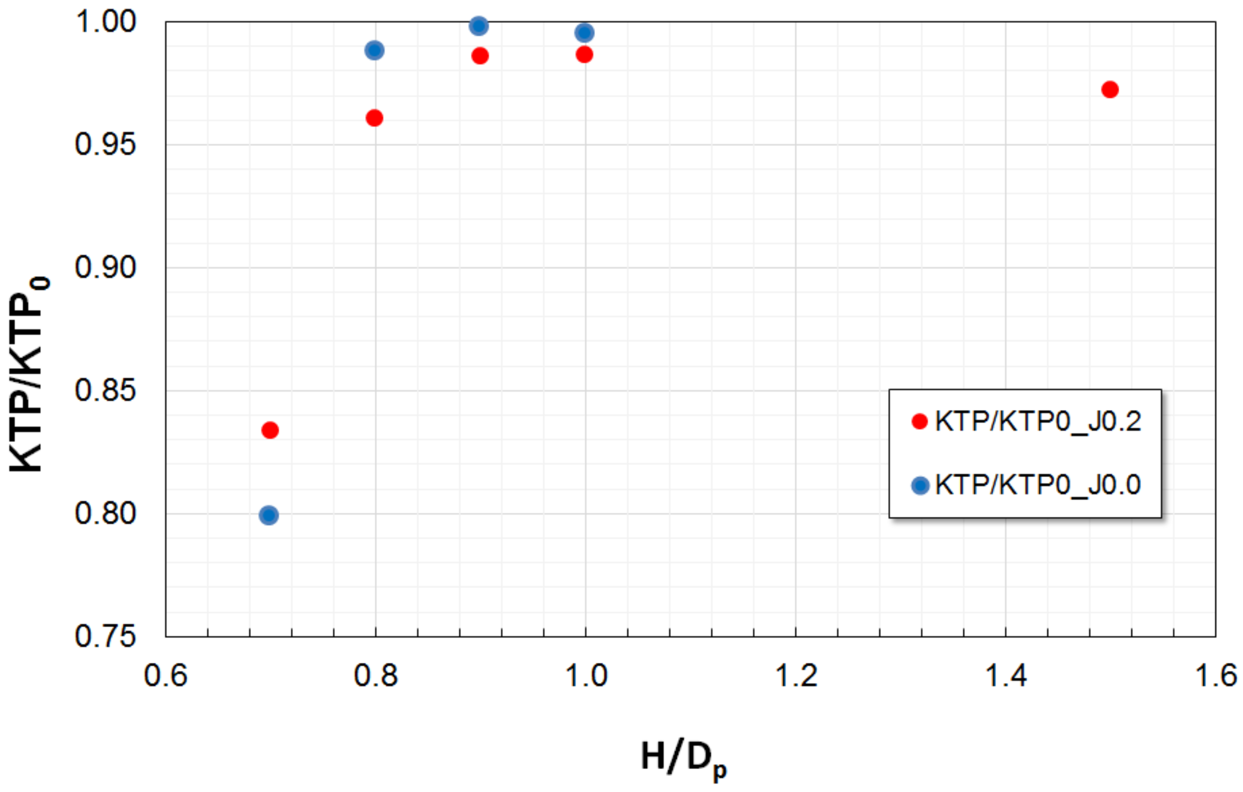
Figure 26.
Variations in propeller thrust, KTP, with propulsor submergence, H/Dp, at J = 0.2 and J = 0.0. (KTP0 refers to the corresponding value in unbounded flow).
Figure 26.
Variations in propeller thrust, KTP, with propulsor submergence, H/Dp, at J = 0.2 and J = 0.0. (KTP0 refers to the corresponding value in unbounded flow).
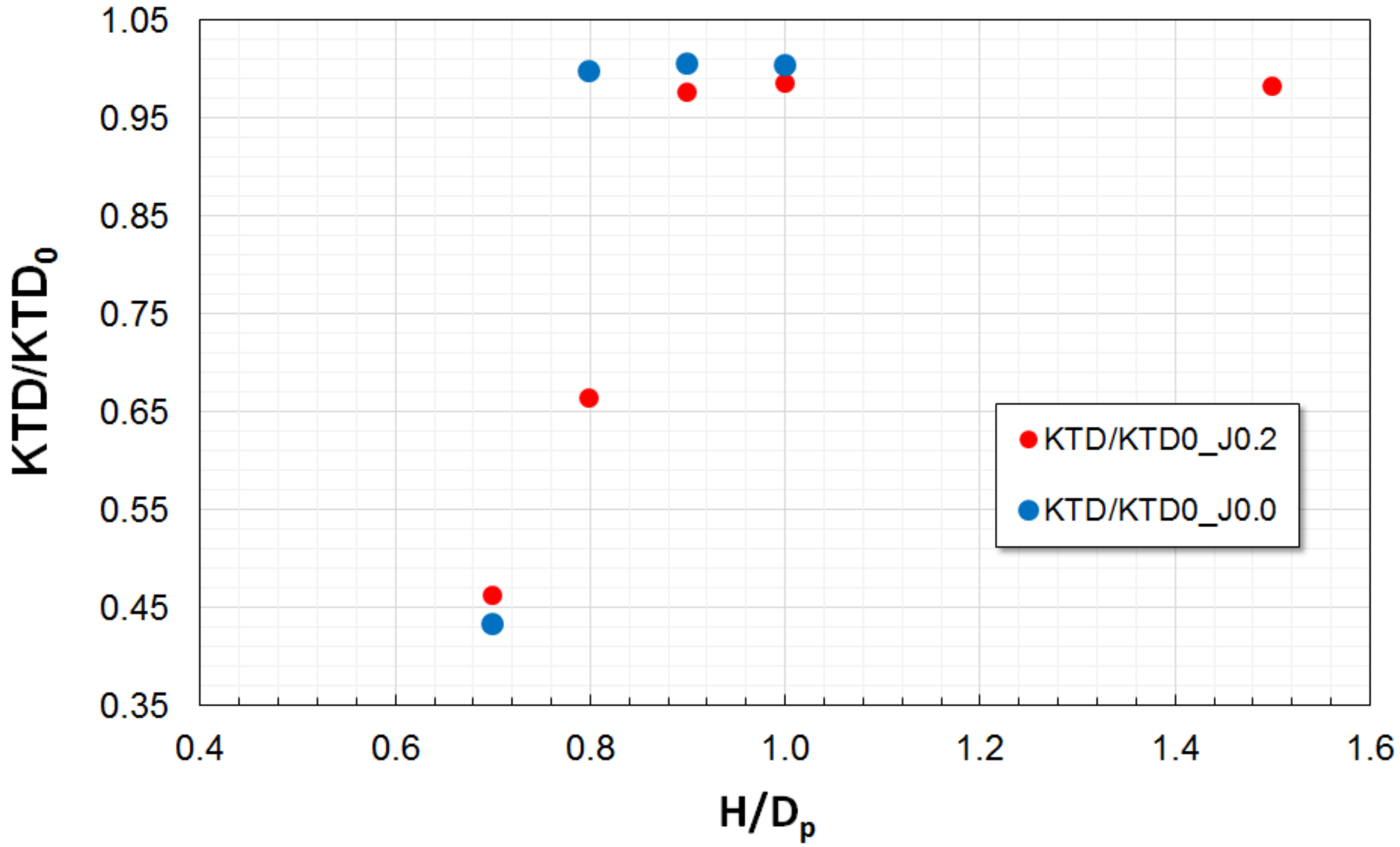
Figure 27.
Variations in propeller thrust, KTD, with propulsor submergence, H/Dp, at J = 0.2 and J = 0.0. (KTD0 refers to the corresponding value in unbounded flow).
Figure 27.
Variations in propeller thrust, KTD, with propulsor submergence, H/Dp, at J = 0.2 and J = 0.0. (KTD0 refers to the corresponding value in unbounded flow).
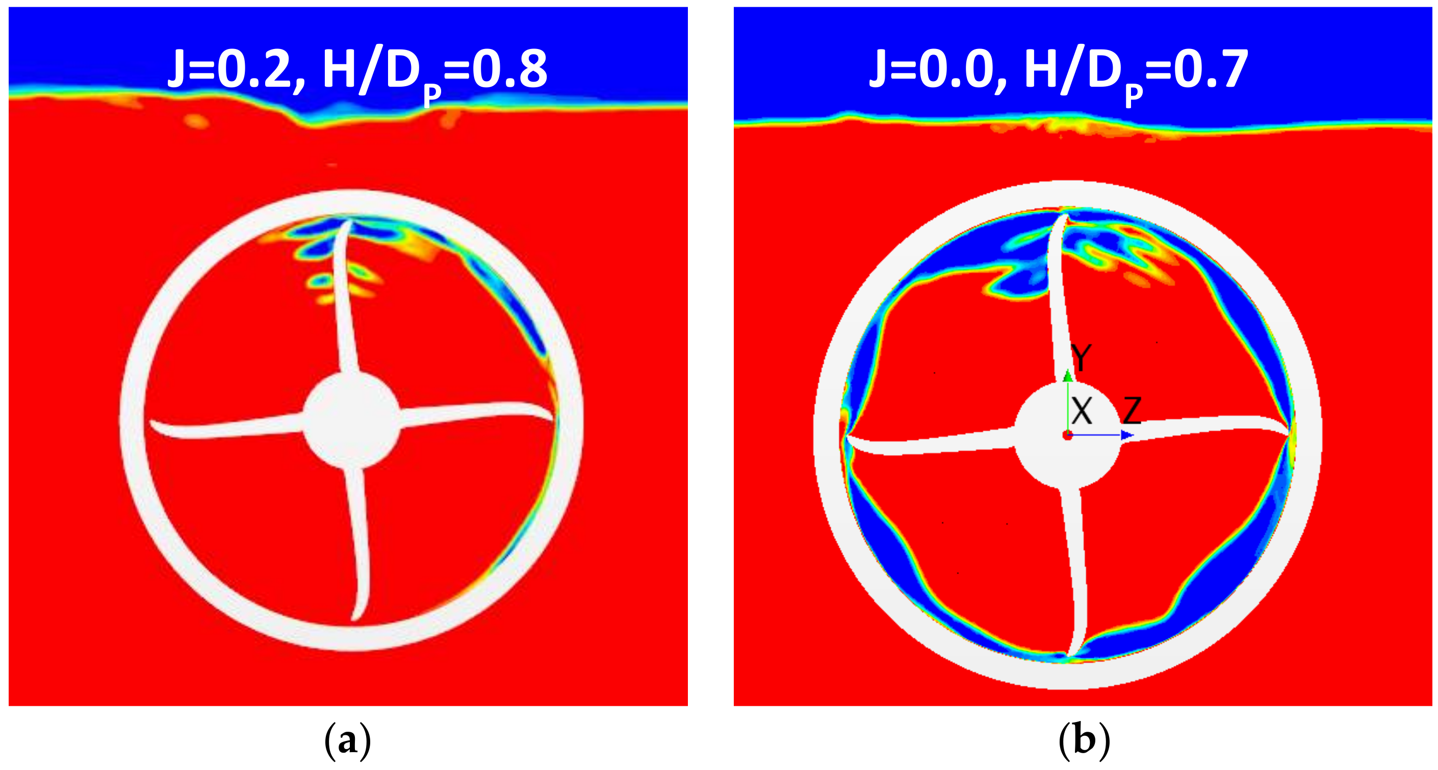
Figure 28.
Contours of volume fraction under fully ventilated conditions at low speed operation conditions: (a) J = 0.2, H/Dp = 0.8; (b) J = 0.0, H/Dp = 0.7.
Figure 28.
Contours of volume fraction under fully ventilated conditions at low speed operation conditions: (a) J = 0.2, H/Dp = 0.8; (b) J = 0.0, H/Dp = 0.7.
Figure 29.
Computed time histories of single blade thrust, KTb, for different magnitudes of submergence, H/Dp, at J = 0.2.
Figure 29.
Computed time histories of single blade thrust, KTb, for different magnitudes of submergence, H/Dp, at J = 0.2.
Table 1.
Main particulars of the tested propulsor model.
Table 1.
Main particulars of the tested propulsor model.
| Thruster Particular | Value |
|---|
| Vertical distance from propeller centre to upper end of strut (mm) | 342 |
| Gondola length (mm) | 181 |
| Strut chord length (mm) | 86 |
| Propeller P-1374 direction of rotation | Right-handed |
| Propeller diameter, Dp (mm) | 250 |
| Hub diameter (mm) | 60 |
| Design pitch ratio, P0.7/Dp | 1.1 |
| Blade skew (degrees) | 25 |
| Expanded blade area ratio | 0.6 |
| Number of blades | 4 |
| Duct type | 19A |
| Duct length (mm) | 125 |
| Duct inner diameter (mm) | 252.78 |
| Blade tip clearance, tc/Dp | 0.0056 |
| Duct max. outer diameter (mm) | 303.96 |
| Duct leading edge radius (mm) | 2.78 |
| Duct trailing edge radius (mm) | 1.39 |
Table 2.
Simulation conditions in oblique unbounded flow.
Table 2.
Simulation conditions in oblique unbounded flow.
| Advance Coefficient, J 1 | Heading Angle (°) |
|---|
| 0.6 (free sailing) | ±60, ±35, ±15, 0 |
| 0.3 (trawling) | ±35, ±15, 0 |
| 0 (bollard) | 0 |
Table 3.
Simulation conditions in presence of free surface.
Table 3.
Simulation conditions in presence of free surface.
| Advance Coefficient, J | Heading Angle (°) | Submergence, H/Dp 1 |
|---|
| 0.6 (free sailing) | 0 | 2, 1.7, 1.5, 1.3, 1.0, 0.9, 0.8, 0.6, 0.5 |
| 0.2 (trawling) | 0 | 1.5, 1.0, 0.9, 0.8, 0.7 |
| 0 (bollard) | 0 | 1.0, 0.9, 0.8, 0.7 |
Table 4.
Measured and computed single blade loads at J = 0.6 for different heading angles.
Table 4.
Measured and computed single blade loads at J = 0.6 for different heading angles.
| | −35° | −15° | 0° | 15° | 35° |
|---|
| Quantity | CFD | EXP | CFD | EXP | CFD | EXP | CFD | EXP | CFD | EXP |
|---|
| KTb | 0.055 | 0.049 | 0.058 | 0.056 | 0.062 | 0.059 | 0.061 | 0.063 | 0.071 | 0.071 |
| σ (KTb) % | 36.4 | 38.9 | 16.8 | 17.5 | 5.8 | 6.3 | 11.6 | 13.1 | 22.1 | 22.0 |
| 10 KQb | 0.071 | 0.086 | 0.075 | 0.089 | 0.079 | 0.098 | 0.078 | 0.095 | 0.087 | 0.087 |
| σ (KQb) % | 24.8 | 23.5 | 12.3 | 12.1 | 4.2 | 4.8 | 8.0 | 8.5 | 15.1 | 19.0 |
| 10 KMYb | 0.021 | 0.016 | 0.021 | 0.015 | 0.019 | 0.008 | 0.020 | 0.011 | 0.016 | 0.012 |
| σ (KMYb) % | 126.3 | 194.4 | 51.2 | 95.7 | 20.6 | 64.9 | 53.6 | 100.1 | 157.6 | 247.0 |
| 10 KMZb | −0.130 | −0.117 | −0.136 | −0.152 | −0.143 | −0.171 | −0.140 | −0.170 | −0.158 | −0.180 |
| σ (KMZb) % | 26.5 | 35.4 | 13.4 | 15.6 | 4.6 | 4.6 | 8.5 | 10.0 | 15.7 | 17.5 |
Table 5.
Measured and computed single blade loads at J = 0.3 for different heading angles.
Table 5.
Measured and computed single blade loads at J = 0.3 for different heading angles.
| | −35° | −15° | 0° | 15° | 35° |
|---|
| Quantity | CFD | EXP | CFD | EXP | CFD | EXP | CFD | EXP | CFD | EXP |
|---|
| KTb | 0.071 | 0.070 | 0.074 | 0.075 | 0.076 | 0.071 | 0.077 | 0.078 | 0.081 | 0.079 |
| σ (KTb) % | 11.9 | 12.0 | 7.1 | 8.0 | 4.0 | 4.7 | 5.3 | 5.6 | 8.1 | 10.8 |
| 10 KQb | 0.087 | 0.099 | 0.091 | 0.096 | 0.092 | 0.112 | 0.093 | 0.108 | 0.097 | 0.101 |
| σ (KQb) % | 8.3 | 9.8 | 5.4 | 6.9 | 3.0 | 3.6 | 3.7 | 4.9 | 5.3 | 9.3 |
| 10 KMYb | 0.014 | 0.008 | 0.012 | 0.001 | 0.012 | −0.006 | 0.011 | −0.004 | 0.010 | 0.000 |
| σ (KMYb) % | 80.8 | 165.2 | 52.1 | 689.6 | 29.2 | 48.4 | 52.4 | 106.2 | 105.9 | 3776.1 |
| 10 KMZb | −0.167 | −0.176 | −0.173 | −0.198 | −0.175 | −0.205 | −0.177 | −0.206 | −0.185 | −0.222 |
| σ (KMZb) % | 8.6 | 9.5 | 5.8 | 6.4 | 3.4 | 3.5 | 4.1 | 5.3 | 5.8 | 8.4 |
Table 6.
Computed single blade loads at J=0.6 for different magnitudes of propulsor submergence.
Table 6.
Computed single blade loads at J=0.6 for different magnitudes of propulsor submergence.
| Quantity | w/o FS | H/Dp = 2 | H/Dp = 1.5 | H/Dp = 1 | H/Dp = 0.8 | H/Dp = 0.7 | H/Dp = 0.6 | H/Dp = 0.5 |
|---|
| KTb | 0.062 | 0.062 | 0.062 | 0.061 | 0.060 | 0.059 | 0.058 | 0.056 |
| σ (KTb) % | 5.8 | 5.5 | 5.7 | 5.4 | 4.5 | 3.6 | 15.0 | 35.4 |
| 10 KQb | 0.079 | 0.078 | 0.079 | 0.078 | 0.077 | 0.076 | 0.073 | 0.067 |
| σ (KQb) % | 4.1 | 4.2 | 4.6 | 4.3 | 3.7 | 3.1 | 14.0 | 34.7 |
| 10 KMYb | 0.020 | 0.020 | 0.020 | 0.021 | 0.021 | 0.022 | 0.011 | 0.000 |
| σ (KMYb) % | 19.8 | 20.2 | 19.9 | 19.6 | 17.5 | 14.5 | 85.5 | 3481.4 |
| 10 KMZb | −0.143 | −0.142 | −0.143 | −0.141 | −0.139 | −0.137 | −0.130 | −0.120 |
| σ (KMZb) % | 4.5 | 4.0 | 4.5 | 4.0 | 3.0 | 2.4 | 17.0 | 40.1 |
Table 7.
Computed single blade loads at J = 0.2 for different magnitudes of propulsor submergence.
Table 7.
Computed single blade loads at J = 0.2 for different magnitudes of propulsor submergence.
| Quantity | w/o FS | H/Dp = 1.5 | H/Dp = 1 | H/Dp = 0.9 | H/Dp = 0.8 | H/Dp = 0.7 |
|---|
| KTb | 0.079 | 0.077 | 0.078 | 0.078 | 0.077 | 0.069 |
| σ (KTb) % | 3.6 | 3.3 | 3.6 | 3.7 | 11.3 | 26.7 |
| 10KQb | 0.096 | 0.093 | 0.095 | 0.094 | 0.090 | 0.077 |
| σ (KQb) % | 2.8 | 2.7 | 3.0 | 3.1 | 11.2 | 28.3 |
| 10KMYb | 0.011 | 0.012 | 0.012 | 0.012 | -0.005 | 0.025 |
| σ (KMYb) % | 25.7 | 24.9 | 26.8 | 30.2 | 203.2 | 52.2 |
| 10KMZb | −0.183 | −0.179 | −0.181 | −0.181 | −0.170 | −0.143 |
| σ (KMZb) % | 3.3 | 2.6 | 3.0 | 3.0 | 13.9 | 33.9 |
