Abstract
Field and numerical investigations at Happisburgh, East coast of England, UK, sought to characterize beach thickness and determine geologic framework controls on coastal change. After a major failure of coastal protection infrastructure, removal of about 1 km of coastal defence along the otherwise protected cliffed coastline of Happisburgh triggered a period of rapid erosion over 20 years of ca. 140 m. Previous sensitivity studies suggest that beach thickness plays a major role in coastal recession. These studies were limited, however, by a lack of beach volume data. In this study, we have integrated the insights gained from our understanding of the Quaternary geology of the area, a novel non-intrusive passive seismic survey method, and a 3D novel representation of the subsurface source and transportable material into a coastal modelling environment to explore the role of beach thickness on the back wearing and downwearing of the cliffs and consolidated platform, respectively. Results show that beach thickness is non-homogeneous along the study site: we estimate that the contribution to near-shore sediment budget via platform downwearing is of a similar order of magnitude as sediment lost from the beach and therefore non-negligible. We have provided a range of evidence to support the idea that the Happisburgh beach is a relatively thin layer perched on a sediment rich platform of sand and gravel. This conceptualization differs from previous publications, which assume that the platform was mostly till and fine material. This has direct implication on regional sediment management along this coastline. The present study contributes to our understanding of a poorly known aspect of coastal sediment budgeting and outlines a quantitative approach that allows for simple integration of geological understanding for coastline evolution assessments worldwide.
Keywords:
erosion; morphodynamic; non-intrusive; downwearing; back wearing; modelling; geological ground model 1. Introduction
Shoreline Management Plans in England envisage implementation of managed realignment along 550 km (ca. 10% of the coastline length) by 2030 [1]. About 66 km of the coastline was realigned between 1991 and the end of 2013. Therefore, an eight-fold increase in the length of realigned shorelines in England is planned in the next decade. Happisburgh, Norfolk on the East coast of England, offers one of the few examples of coastal defence removal. From this example we can learn some lessons about the role of the geologic framework controlling coastal change, when transitioning from hold-the-line approaches to managed realignment approaches.
The average rate of erosion at Happisburgh between 1885 and 1907, measured from historical maps, was 0.8 m/yr and approximately 0.4 m/yr between 1907 and 1950 [2]. The average erosion rate after the removal of the defences is the order of 7 to 17 times larger than annual average erosion rates before the construction of the defences.
A plausible explanation (or hypothesis) for post-removal increase in erosion rate is that the discontinuity in the platform lowering rates across the line of the defence drives the rapid erosion after this defence is lost [3]. Figure 1 illustrates the stages through which these processes may occur. Sensitivity testing [3] suggests that the beach thickness is a key factor in determining the scale of response, and whether there is a net gain or loss of land when more natural conditions have re-established. A reduction in beach volume following defence construction leads to a thinning of the beach, and so an increase in wave-driven platform downwearing and the accelerated development of a step. Such a reduction in beach thickness may reasonably be expected to have occurred at Happisburgh when the defences were built, simply because the beach received less sediment as a consequence of a reduced rate of cliff recession. If this hypothesis is realistic then it suggests that, in some settings, the presence of coastal protection can ultimately result in a net loss of land. This would have important implications for coastal management including: (1) new defences may be seen as detrimental because of the decommissioning losses (so long as those are accounted for) but conversely; (2) decisions to maintain existing defences may become more likely, because of the increased losses that would result from their decommissioning. The analysis presented by [3] is lacking any data of beach thickness and contains little direct evidence of accelerated platform lowering. Platform lowering is difficult to observe at the study site (and in many places) during storms due to the harsh conditions and, during calm weather, because contemporary beach deposits lie on top of the shore platform. The aim of this work is to examine this hypothesis.
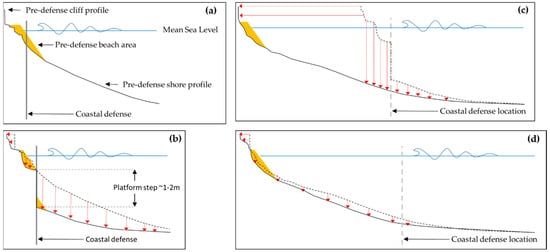
Figure 1.
Illustration of the development and loss of a step in the shore platform profile due to the construction and removal of a vertical coast protection. Beach volume is represented as a yellow polygon and shore platform profile as a black solid line. The panels show an idealized beach and shore platform evolution; (a) initial beach and shore platform profile at the time of construction of the coastal defence; (b) after the construction of the defence, shore platform lowering (red arrows) seaward of the defence is larger than behind, and so a step develops; (c) when the defence is removed, the (steepened) shore platform previously behind the step is exposed to higher wave energy, inducing rapid shore platform and cliff retreat (the shore platform in front of the structure continues to erode at a low rate); (d) after a period of time the step is removed and a new quasi-equilibrium coupled beach and shore platform profile is reached; retreat rates then reduce and become more steady; (e) sensitivity analysis has shown that the ‘overtake’ (i.e., excess net shoreline retreat caused by this process) increases if beach volume decreases.
This work is an extension of the preliminary results presented by [4]. Here we combine field observations with our understanding of the Quaternary geology of the study site within a novel coastal landscape evolution numerical framework. This enables us to estimate the beach thickness at the time of defence removal, and to assess any changes in beach volume and shore platform elevation over time.
2. Study Site
Happisburgh is a village situated in North Norfolk, on the soft sediment coasts of eastern England (Figure 2). Sea levels at this location have been rising for millennia [5], and under natural conditions, the coast of Norfolk is erosional. In response to the 1953 flooding, a continuous line of defences was constructed in the 1960s to protect the village, extending 15 km from Happisburgh to Trimingham to the northwest (Figure 2). These comprised sheet piles, crested with a sloping timber palisade, fronted by groins. The design was intended to reduce cliff recession rather than entirely prevent it, and to allow some sediment to sustain the beaches. Since 1996 the Environment Agency (EA) have undertaken a series of beach nourishments (around 150,000 m3/yr on average [6]) at Sea Palling, about 5 km to the south and down-drift of Happisburgh. The nourishment scheme aims to offset the concomitant reduction in sediment supply from cliff erosion along the Happisburgh–Trimingham coastal section, and to maintain sea defence. In the early to mid-1990s, deterioration of the Happisburgh structures led to their progressive failure. Sheet piles were buckled and palisades and groins were broken and destroyed by wave action. This led, very rapidly, to the formation of an embayment, partially stabilized at its northern end by a series of placements of a rock armour revetment. The EA [3] report that, following structure failure, up to 140 m (7 m/yr) of recession occurred within the Happisburgh embayment between 1992 and 2012.
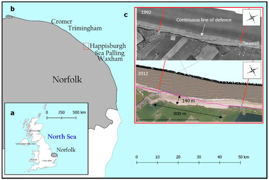
Figure 2.
Study location: (a) Happisburgh is located in county of Norfolk (grey polygon) on the east coast of England, the grey lines represent the administrative boundaries of the different UK regions; (b) study site location (red rectangle) and nearby locations mentioned on this manuscript; (c) aerial images of Happisburgh taken in 1992 and 2012 by the Environment Agency; showing the formation of an embayment. Red lines indicate the location of profile monitoring surveys, and the magenta line shows the approximate cliff toe position in 1992.
The site is fully exposed to Southern North Sea waves, with average annual significant wave heights (Hs) of 0.9 m and peak periods (Tp) of 4 s from the N-NNE (Figure 3a), obtained from the UKCP09 downscaled data [7] for the period 1961-2016 at a point located at 2.5 km offshore and 20 m depth. The wave climate is non-seasonal with similar moderate-energy summers (July to September, Hs = 0.95 m and Tp = 4 s) and moderate-energy winters (October to June, Hs = 0.92 m and Tp = 4 s), and extreme wave heights exceeding Hs = 6 m and Tp = 10 s. The coast is macrotidal, with a mean spring range of 4.23 m and mean neap range of 2.09 m, obtained from the observed tidal elevations at Cromer during the years 2008 to 2026 (http://www.ntslf.org/tides/hilo). Cromer is the nearest tide gauge station, located about 20 km north of Happisburgh. The top 10 skew surges (i.e., the difference between the maximum observed sea level and the maximum predicted tide) registered at Cromer varies from 1.76 m to 1.13 m and occurs during the winter months of November, December, January and February (data from National Oceanography Centre, http://www.ntslf.org/storm-surges/storm-surge-climatology/england-east). The largest skew surge was registered in 21 February 1993 06:15, causing considerable erosion along the coastline. At Happisburgh a large portion of the south cliff was swept away causing a bay to be formed and farm land lost (cited from http://www.happisburgh.org.uk/ccag/history). In the Southern North Sea region, peak wind speeds are predominantly in the range of 28.5 to 32.7 m/s (Beaufort Force 11) and coming from the west, and the most likely wind direction is from the SW and W [8].
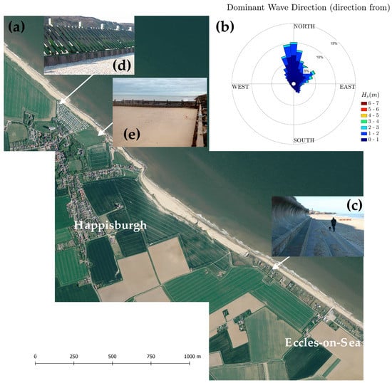
Figure 3.
Study site: (a) aerial view of the study region in 2010 showing the embayment (source EA, year 2010); (b) wave rose for Happisburgh created using downscaled data (1961–2016) from the UKCP09; (c) detail of the sea-wall protecting the low-lying coast of Eccles-on-Sea; (d) view of the wood revetment and sheet pile that is still in place northwest of Happisburgh (source Mike Walkden, year 2013); (e) detail of wooden groin used to slow down the alongshore sediment transport (source Andres Payo, 2017).
Defences were constructed in 1958/1959 (wooden revetments and steel sheet piles) and 1968 (wooden groins) [9,10] (Figure 3d,e) on the soft cliff coastline which formerly eroded at less than 1 m/yr [10]. The steel sheet piles are at the landward limit of the groins that lie perpendicular to the coast with a length of 100 m and are evenly spaced along the coast every 170 m. After construction of the defences, the rate of erosion decreased, and any subsequent loss of land was caused by failure of unstable cliff slopes. From the late 1980s, the defences were not maintained, in part because of a lack of agreement regarding coastal protection, and in part because a lack of funding [9]. By 1991, defence failure led to selective defence removal on safety grounds along 900 m of coast [10], while adjacent defences remained. Subsequently, where defences were removed, excessive retreat occurred and, over a period of 14 years, the cliff eroded on average 100 m landward, creating an embayment. Between September 2001 and September 2003, 3.6 × 10⁴ t of sediment was eroded from a 100 m section of cliff [11] with retreat rates recorded between 8 and 10 m/yr. In 2007, with financial help from the local authority, the local community helped fund rock armouring along the cliff base to slow the erosion [12]. The adjacent and still defended coasts currently form promontories along the coast. At the southern end of the embayment, a sea-wall protects the low-lying farmland and tourist area of Eccles-on-Sea. This sea-wall was constructed after catastrophic floods in 1953 in stages up to 1987, and there are now three main elements making up the sea defence system: the beach, the sea wall and the sand dunes [6]. The beach becomes highly mobile during storms, and can be drawn down to such an extent that the sea wall becomes unstable. In the early and mid-1990s, beaches in the Eccles/Sea Palling area reached critical levels where the sea wall foundations started to fail. Three emergency works contracts were implemented for placing rock protection along the toe of the sea wall. If the sea wall was allowed to collapse, the sand dunes would offer the last line of defence and would be breached rapidly by wave action [6].
The cliffs at the study site range in height from 6 to 20 m above Ordnance Datum (OD). They are composed of a sequence dominated by glacigenic sediments including multiple diamictons (admixtures of poorly-sorted clay, sand and gravel), separated by beds of stratified silt, clay and sand (Figure 4) [13,14,15]. These units were deposited during several major incursions of glacier ice into the region during the Middle Pleistocene [16]. The basal unit that discontinuously outcrops at the base of cliffs is the Crag Group (Early to early Middle Pleistocene age), which is typically obscured by modern beach material but is periodically exposed following storms [11]. The Crag Group consists of stratified sands and clays interpreted as shallow marine to inter-tidal in origin andvpunctuated by occasional elongate lens-shaped bodies of fluvial muds [17,18]. The Crag Group rests unconformably on an undulating upper surface of cchalk bedrock (Cretaceous age). chalk bedrock depths increases from about −25 mOD at the northern end to −40 mOD at the southern end. The large potential stock of sand and gravel at the shore platform associated with the Crag Group suggest that the beaches at Happisburgh might not be sediment starved, providing that the wave and currents have enough energy to erode and transport this material towards the coast.
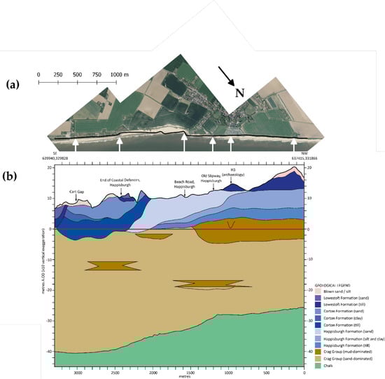
Figure 4.
Main geological units at the study site along the 1999 cliff top line: (a) cliff top line of year 1999 is shown as solid black line on top of year 2010 aerial photography of the study site; (b) main lithological units. Key landmarks along the cliff cross section are named in (b), approximate locations on (a) are indicated by white arrows. Across-shore distances are distances measured along the cliff top line (starting at the northern end) and vertical elevation are relative to Ordnance Datum (which is approximately at mean sea level for the study site). For clarity, the vertical scale has been exaggerated 10 times.
3. Materials and Methods
3.1. Field Observations
3.1.1. Passive Seismic Survey
We used a passive seismic survey method to search for evidence of platform lowering in front of and behind the existing coastal defences and to build confidence in the subsurface lithological model. Passive seismic surveys measure background seismic noise (both natural <1 Hz and man-made >1 Hz) to estimate the thickness of the different lithologies through different time domains and spectral techniques. Seismic tremor, commonly called seismic ‘noise’, exists everywhere on the Earth’s surface. It mainly consists of surface waves, which are the elastic waves produced by the constructive interference of P and S waves in the layers near Earth’s the surface. Seismic noise is mostly produced by wind and sea waves. Industries and vehicle traffic also locally generate tremor, although essentially at high frequencies (>1 Hz), which are readily attenuated. Passive seismic surveys consist of a series of single-station point recordings, generally arranged into linear transects. These can be of any length and, where organized into an appropriate grid pattern, can be used to generate 3D surfaces of target horizons. Best results are achieved where independent depth control—such as borehole information—is available to calibrate the results. We used the Tromino ENGY-3G (moho.world/tromino) a small (10 × 14 × 8 cm), portable (~1 kg), broadband, three-component seismometer and the proprietary software Grilla (v7.0) that implements the Horizontal-to-Vertical Spectral Ratio (H/V) method [19,20]. The reason behind using the spectral noise ratio is that seismic noise varies largely in amplitude as a function of the noise “strength” but the spectral ratio remains essentially unaffected and is tied to local subsoil structure [21]. The Grilla software also provides routines for quality control of the H/V analyses following the European SESAME project directives [22].
Seismic ground noise acts as an excitation function for the specific resonances of the different lithologies in the subsoil. For example, if the subsoil has proper frequencies of 0.8 and 20 Hz, the background seismic noise will excite these frequencies making them visible when applying the H/V technique on the recordings and these proper frequencies can be used as a proxy for cover thickness. In simple double layer stratigraphy sedimentary (cover + bedrock), there is a simple equation [23] relating the resonance fundamental frequency f0 to the thickness h of the layer and Vs (the shear wave velocity in the same layer):
where the value of Vs varies for different materials with typical values of: 100–180 m/s for clay, 180–250 m/s for sand and 250–500 m/s for gravel. In case of several peaks on the H/V curve, the peak with the lowest frequency is the fundamental mode (f0, generally the bedrock-cover limit) and other peaks (i.e., f1, f2, …, fn) correspond to other geological limits which also cause seismic motion amplification. For the stations located on the beach at the study site we would expect to see one peak corresponding with the interfaces between the Crag Group and the chalk (f0), one peak at the interface between the contemporaneous beach deposits and the Crag Group (f1) and one non-lithological peak corresponding to the presence of the sheet pile (Figure 5). The estimated frequencies for f0 and f1 are based on the borehole observations at the study site, indicating that the chalk surface is at a depth of ca. −20 m OD and maximum VsVs velocities is on the order of typical sand deposits and gravel deposits. If the impedance (density × Vs) difference between the contemporaneous beach deposit and the Crag Group is large enough, and assuming beach elevation is equal in front of and behind the palisade, we will expect to see a decrease on the f1 frequency (i.e., increasing depth) as we compare the H/V ratios behind and in front of and behind the palisade.
f0 = Vs/(4h),
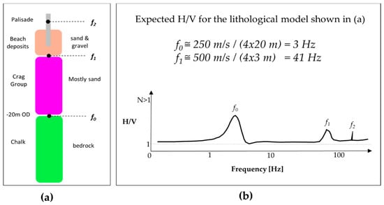
Figure 5.
Expected spectral noise Horizontal to Vertical (H/V) ratio for the assumed lithological model on the beach at Happisburgh; (a) lithological model showing the main lithologies, their composition (i.e., sand, gravel, bedrock) and the expected peak frequencies; (b) expected H/V and approximated values of the lithological peaks f0 and f1. The f2 peak is an expected non-lithological signal (i.e., sharper than lithological peaks) resulting from the man-made coastal defence.
Based on the expected H/V (Figure 5), the Tromino was setup to measure background noise during 4 min at 1024 Hz sampling frequency. According to the Nyquist theorem, the highest frequency that can be recovered from a digitized signal is always lower than half the sampling frequency. Hence, sampling at 1024 Hz one can resolve signals at frequencies at most 512 Hz high. For a sand and gravel beach deposit (max Vs ~ 500 m/s) of thickness O (1 m to 0.5 m), we will expect f1 peak to be around 125–250 Hz, which is well within the maximum observable frequency when sampling at 1024 Hz. In practice, spectral estimates are statistical in nature and, to have stable results, the observation time should be long enough to comprise at least 10 repetitions of the longest period of interest. For our study, the longest period (T0) (i.e., lower frequencies) correspond with f0 ~ 3 Hz (T0 ≅ 1/3 = 0.33) which means 10 × 0.33 = 3.3 s. Because we are going to extract information from seismic noise, we expect fluctuations with time, which can be appropriately controlled by sampling a number N of 3.3 s windows sufficient to compute an average that is statistically significant. Common practice shows this number N to be 30–50, which means in the above example a total recording time of 50 × 3.3 = 165 s = 2.75 min. A total length of four minutes was then considered long enough for this study.
A one-day passive seismic field survey was conducted on 24 October 2017 (Figure 6). A total of 34 points were measured along five transects perpendicular to the coast-line. On each transect, the measurements points were equally spaced (every 10 m) from the cliff toe to the seaward limit of the dry beach at the time of the survey. Four extra points were recorded at the northern side where beach levels were similar in front of and behind the palisade and beach elevation in front of the palisade was larger (>1.5 m) than on the transects. The large difference in beach elevation is due to the damaged groin located at the southern side of line 5 that was not retaining beach sediments effectively. On the day of the survey the weather conditions were mild; moderate winds (gust velocities < 10 m/s) blowing from the east and no wave activity (Hs < 0.25 m). Wind did not affect the recordings at the beach, which was protected by the cliff. The survey was conducted by a two-person team. Data recording started at 12:39 p.m. and finished at 15:41 p.m. (~3 h). The points of the stations were located using a handheld Garmin GPS (GPSMAP 64 s) on which the planned locations were pre-loaded as waypoints. During the survey, one of the team members was in charge of navigating to the waypoints and marking with pegs the approximate locations. The second team member was in charge of recording with the Tromino and annotating the relative distance to the palisade for further reference. The Tromino unit was coupled to ground at each point using three 6 cm long spikes (~4 cm penetration length). The coupling was achieved by alternately pressing on the lowermost corners of the box and on the middle of the top edge to set Tromino in a horizontal position (e.g., until the air bubble in the spirit is positioned at the centre of the level). Caution was taken to avoid creating any non-coherent noise while recording.
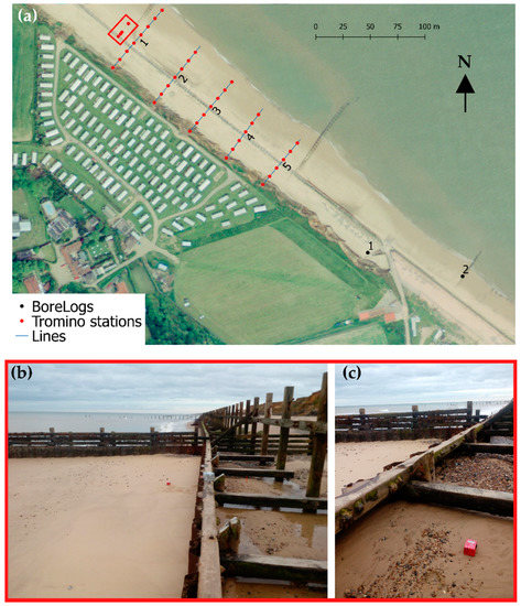
Figure 6.
Passive seismic survey recorded locations; (a) 34 points along five lines (i.e., lines 1 to 5) were initially recorded covering the beach from the cliff toe to the seaward limit of the dry beach. Four additional points were recorded during the day, these are shown as points within a red rectangle; (b) detail of the extra station recorded immediately in front of the palisade and; (c) detail of extra station recorded immediately behind the palisade. Beach levels on stations shown in (a,c) were similar within ±10 cm.
3.1.2. Digital Terrain Model of Study Area
A seamless Digital Terrain Model (DTM) of the inland topography and near-shore bathymetry of the study site is required to build the 3D subsurface lithological and thickness model. Here, we have combined different sources of data provided by the EA under the Open Government Licence: the Light Detection and Ranging (LIDAR) data from 1999 for the inland topography and the multibeam bathymetry data for 2011. The inland topography and bathymetry data are available to download from https://data.gov.uk/dataset (LIDAR 1999 at /lidar-dtm-time-stamped-tiles and the multibeam at /multibeam-bathymetry). LIDAR is an airborne mapping technique, which uses a laser to measure the height of the terrain and surface objects on the ground such as trees and buildings. Hundreds of thousands of measurements per second are made of the ground allowing highly detailed elevation models to be generated at spatial resolutions of between 25 cm and 2 m. The EA-LIDAR DTM time stamped tiles product is a ‘bare earth’ model with surface objects filtered out from the Digital Surface Model (DSM) by applying bespoke software techniques to leave the best representation of the terrain. All EA-LIDAR data has a vertical accuracy of ±15 cm RMSE (Root Mean Square Error). The EA-LIDAR data are supplied in OS GB’36 British National Grid, with elevations recorded above Ordnance Datum Newlyn (AODN). The EA-LIDAR data are supplied as individual ASCII files labelled by Ordnance Survey grid reference. The DTM product is available at 2 m, 1 m, 50 cm and 25 cm horizontal resolutions: for this work we used the 2 m resolution DTM. Multibeam echo sounders, for bathymetric survey, use sonar pulses to measure the distance between the survey vessel and the seabed. This instrument collects point data at a horizontal resolution of 25 cm or better, depending on water depth, vessel speed and bed topography and produces a high-resolution elevation dataset of the underwater terrain. Multibeam data are available at 50 cm horizontal resolution and supplied as an ESRI ASCII Raster, which contains height relative to Ordnance Survey Newlyn datum. Elevation values are in meters. The closest time-stamped LIDAR and multibeam dataset to the removal date of coastal defences (1991/1993) was 1999 for the inland topography and 2011 for the bathymetry (Figure 7a). This combined data set has some gaps along the coast, where water depth is too shallow for the vessels operating the multibeam to obtain good quality data and therefore outside the reach of the LIDAR. To produce a seamless DTM interpolation was required.
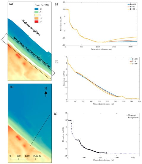
Figure 7.
DTM of study site: (a) EA-LIDAR inland topography year 1999 and EA-multibeam bathymetry year 2011 (white areas indicate data gaps); (b) interpolated DTM used in this work; (c) comparison of elevations along the transect shown by a solid black line in (b) using different tension parameter values (i.e., notice the unrealistic depth decrease seawards of ca. 1250 m cross-shore location); (d) detail of the upper shore-face interpolated bathymetries for different tension parameter values; (e) the final interpolated elevation along the same transect.
We created a seamless DTM by interpolating the combined LIDAR and multibeam datasets (Figure 7b). Before the interpolation, both datasets were resampled to a 5 m raster cell resolution. For the resampling, and posterior interpolation, we have used the SAGA toolbox [24] for QGIS (2.18.3 for Windows, https://qgis.org/). The resampling was done using SAGA-Resampling using the nearest-neighbour interpolation method to upscale. For the interpolation we have used the SAGA-Close Gaps function with a tension threshold of 0.1. The Close Gaps function uses a method commonly called minimum curvature under tension to interpolate the missing data [25]. The method interpolates the data to be gridded with a surface having continuous second derivatives and minimal total squared curvature. The minimum-curvature surface has an analogy in elastic plate flexure and approximates the shape adopted by a thin plate flexed to pass through the data points. Minimum-curvature surfaces may have large oscillations and extraneous inflection points which make them unsuitable for gridding in many of the applications where they are commonly used. These extraneous inflection points can be eliminated by adding tension to the elastic-plate flexure equation [25]. The tension parameter (T) is a user-defined value that varies from 0 to 1: T = 0 is equivalent to the minimum curvature solution and T = 1 forces the solution to flatten at the edge. We have compared the seamless DTM using T = 0.01, 0.1 and 0.9 (Figure 7c) and found that the results T = 0.01 produced more realistic interpolated bathymetries in the near-shore (Figure 7d). For the offshore bathymetry none of the tension parameters tested produced a good extrapolation; all interpolated DTM showed values of unrealistic elevation rise seaward. The offshore data gaps were filled by simple interpolation using the nearest-neighbour method that produces a more realistic flattened offshore bathymetry (Figure 7e).
3.2. Numerical Modelling
3.2.1. 3D Subsurface Model
A 3D geological model of the Quaternary sediments in the area was constructed using GSI3DTM software (version 2013) [26]. GSI3DTM combines a digital elevation model, surface geological line-work and down-hole borehole and geophysical data to enable the geologist to construct cross sections by correlating boreholes and the outcrops to produce a geological fence diagram. Mathematical interpolation between the nodes along the drawn sections and the limits of the units produces a solid model comprising a stack of triangulated objects each corresponding to one of the geological units present. Geologists generate cross-sections based on facts such as borehole logs informed by experience.
All 29 BGS-held borehole logs within 1.5 km of the study area were assessed for suitability for modelling. Together with the corresponding 1:50,000 scale geological map, a total of 16 boreholes constrain a mesh of 38 manually correlated cross-sections. The coastal cliff section illustration shown in Figure 4 was used as the backdrop to a modelled cross-section along the same route. This was the first cross-section to be correlated and forms the basis of the entire model (Figure 8a).
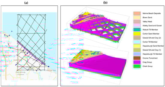
Figure 8.
Happisburgh 3D lithological model; (a) distribution of boreholes (blue circles) and cross-sections (black lines) used to construct the model, master coastal cross-section is highlighted in magenta; (b) upper panel shows all the cross sections with its interpreted geology and bottom panel shows the interpolated 3D lithological model.
Coverages representing each of the 14 modelled geological units were constructed using mapped outcrops and the distribution in the cross-sections. These unit coverages were modified using the DTM because the coastline has changed since the area was surveyed. For example, the break of slope at the base of the cliff has an elevation of 3 m above sea level. This elevation was used to re-shape the landward edge of the marine beach deposits. Similarly, the break of slope at the top of the cliff was used to refine the distribution of blown sand. This corrected for beach deposits ‘climbing’ up the cliff and blown sand draping onto the foreshore.
GSI3DTM calculates the elevation of the top and base of each geological unit and its thickness by triangulating between digitized nodes along the cross-sections and nodes around the edges of unit coverages. These tops, bases and thicknesses were exported from the model as ASCII grids with a cell size of 5 m. The model is capped by the DTM described in Section 3.1.2. and has a nominal cut-off depth of 50 m below Ordnance Datum.
Standard QA checks are carried out on all BGS 3D geological models prior to publication. This includes ensuring that unit bases are ‘snapped’ at crossing points in the cross-sections and artefacts such as spikes are investigated. ‘Helper sections’ are added to improve the calculation of specific geological units, such as those with irregular or linear distribution patterns. In the Happisburgh model a number of helper sections were added to improve the calculation at the cliff edge.
3.2.2. Landscape Evolution Modelling: CoastalME
We numerically explored the contribution of platform downwearing to the nearshore sediment budget using the Coastal Modelling Environment (CoastalME) [27]. CoastalME is a modelling environment to simulate decadal and longer coastal morphological changes. The rationale behind CoastalME is to capture the essential characteristics of the landform-specific models using a common spatial representation within an appropriate software framework. CoastalME can be used to integrate the Soft Cliff and Platform Erosion model SCAPE, the Coastal Vector Evolution Model COVE and the Cross Shore model CSHORE [27]. This model combination (SCAPE + COVE + CSHORE) captures the main processes and feedbacks required to simulate the beach-platform-wave propagation interaction that drives coastal morphological change at Happisburgh. Table 1 summarizes the main methods and what element has been implemented in CoastalME [28].

Table 1.
Component model, description and what element is implemented in CoastalME.
Input parameters for CoastalME are supplied via a set of raster, vector, and text-format time series files and a text-format configuration file. Raster files represent the initial ground elevation, sediment thickness and coastal intervention. Vector files contain the locations within the model’s spatial domain for which wave (wave height, direction and period) time series are provided as text files. Tidal elevation is also provided as a time series text file. CoastalME’s output consists of GIS layer snapshots, a text file, and a number of time-series files. The GIS files include both raster layers such as digital elevation models (DEMs) and sediment thickness, and vector layers such as the coastline. Here, we outline the main steps followed to apply this modelling environment to the Happisburgh case. The steps followed to simulate the Happisburgh landscape evolution are:
- Initialize the thickness model: The DTM and lithological model are converted into a raster thickness model that represent the ground elevation and the consolidated and non-consolidated stock of coarse, sand and fine material in the subsurface.
- Define the intervention type and its above–ground elevation: The existing coastal defences (i.e., palisade and sea wall) are digitized and represented in a raster file. Raster cells marked as an intervention type are assumed not to erode over time. In addition to the location, the intervention has an assigned above-ground elevation that allows the model framework to assess if it is submerged or not at different tidal phases.
- Characterize the driving forces and resistance forces: for this exploratory assessment, we have assumed an idealized wave climate that represents the main drivers of coastal morphological change in the area. In particular, we have assumed a constant wave height, wave period and wave direction that roughly correspond with the net annual energy flux and we vary the tide level every hour according to the tidal harmonics registered at the nearby tide station in Cromer. The resistance cliff downwearing has been assumed equal to the cliff back wearing resistance and was calibrated to reproduce the observed cliff erosion between 1999 and 2004.
The smallest spatial element within CoastalME is a block; blocks are square in plan view and of variable thickness. A coastal stretch is characterized by a minimum of two raster input files. These are (1) a basement file giving the elevation of non-erodible rock that underlies; (2) a single sediment layer giving the thickness of a single sediment size fraction, either consolidated or unconsolidated. Whilst the basement is a non-erodible layer, consolidated and unconsolidated sediment layers may increase or decrease their thickness during a simulation. Each sediment layer potentially comprises three size fractions, fines (mud/silt), sand (0.063 mm < D50 < 2.0 mm) and coarse (2.0 mm < D50 < 63.0 mm) sediment; however, any of these size fractions may be omitted for some or all raster cells, in which case the model will assume zero thickness of this size fraction for that raster cell. Non-consolidated layers are assumed to lie above consolidated sediment layers, and the size fractions within a layer are assumed to be well mixed within that layer. Consolidated sediments are essentially erodible solid rock while unconsolidated sediments are loose materials, ranging from clay to sand to gravel. Sediment grain sizes for both consolidated and unconsolidated layers are specified in the configuration file (the default assumed values of different fractions sediment size is 0.065 mm, 0.42 mm and 19.0 mm for fine, sand and coarse respectively). The sediment mass transferability between these six different types of sediment (three sediment size fractions and two consolidation states) is hard-coded within the CoastalME framework. Consolidated coarse and sand sediment fractions, when eroded, are assumed to become part of the unconsolidated coarse and sand material. In the present version of the model, eroded fine material is simply assumed (as in SCAPE) to become part of a global suspended sediment fraction (i.e., not lost but stored as suspended sediment). The elevation of the sediment top elevation or DEM is obtained by summing layer thicknesses to the elevation of the basement. The method used to convert the lithological model into a CoastalME thickness model is novel and described in detail in the next section.
3.2.3. Converting 3D Lithological Model into CoastalME Thickness Model
Using empirical knowledge supported by data from the BGS National Geotechnical Database [33] the lithostratigraphical units expressed in the model were assigned average percentages for fines (<0.63 mm), sand (0.63–2 mm) and coarse material (>2 mm) (Table A3 in Appendix B). The chalk consists mainly of silt particles which although it forms a consolidated rock was added to the fines fraction, equally all organic material was considered to be part of the fines fraction. A GS3DTM script was used to query the geological model across a 50 × 50 m grid to calculate the average grain size distribution of the geological sequence at each grid cell. The resulting data was converted into a format suitable for use by CoastalME.
4. Results
4.1. Passive Seismic Survey Results in Front and behind the Defences
Figure 9 shows the noise (in non dimensional H/V units) time series recorded and selected to calculate the H/V spectral ratio at the seaward and landward side of the palisade. A coherent noise was recorded at the frequency band between 1 Hz and 10 Hz at both locations (Figure 9b,e). Sporadic noise at frequencies lower than 0.5 Hz were manually removed from the analysis (Figure 9c,d), keeping the remaining 85% and 75% of the record at the seaward and landward side respectively.
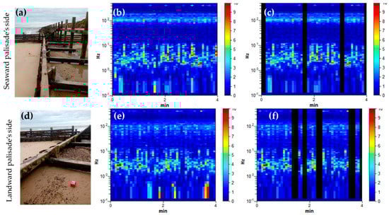
Figure 9.
Noise time history recorded and used to calculate the H/V spectra at both sides of the palisade: (a) location of the Tromino at the seaward side of the defence; (b) full record measured at the seaward side; (c) non-used noise data at the seaward side masked with black; (d) location of the Tromino at the landward side of the defence; (e) full record measured at the landward side; (f) non-used noise data at the landward side masked with black;.
Figure 10 shows the measured and synthetic N-S/V spectral ratio, and single component spectra at the seaward and landward side of the palisade. We calculated the spectra for each directional component using a window size of 5 s, and 5% smoothing using a triangular window. The maximum of the N-S/V spectral ratio was found equal to 2.5 ± 0.29 Hz and 2.75 ± 0.25 Hz for the seaward and landward side of the palisade. This frequency corresponds to the interface between the Crag Group and the chalk bedrock. According to the SESAME guidelines, all the three criteria for a reliable H/V curve are fulfilled at both sides but only four out of six (i.e., rather than five out of six) criteria for a clear peak are fulfilled again at both sides (Table A1 and Table A2 in Appendix A). We modelled (synthetic H/V curve in Figure 10a,c) the subsurface as a single cover layer over the bedrock assuming a Vs of 250 m/s, and Poisson ratio of 0.42 for the top cover and 560 m/s and Poisson ration of 0.35 for the bedrock. The synthetic model suggests that the thickness of the cover layer is 27 m and 24 m at the landward and seaward sides respectively, this is of the same order suggested by nearby borehole data. Notice that we have used the N-S/V (North-South component to vertical component ratio) instead of the average of the two horizontal components (N-S and E-W) because the N-S and E-W spectra are significantly different at frequencies larger than 100 Hz, where we will expect to see the platform lowering. As the Tromino unit was always oriented with the N-S component pointing to the alongshore dimension of the beach, we have assumed that this component is less affected by the across-shore non-uniformities due to the presence of the cliff and/or the presence of a platform step.
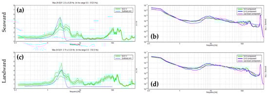
Figure 10.
N-S/V spectral ratio, synthetic N-S/V and single component spectra at the seaward and landward side of the palisade; (a) measured (green lines, where thick line is the average and thin lines are the standard deviation) and synthetic (blue line) N-S/V spectral ratio at the seaward side; (b) directional components spectra at the seaward side; (c) measured (green) and synthetic (blue) N-S/V spectral ratio at the landward side; (d) directional components spectra at the landward side.
4.2. Beach Thickness Along-Shore Variability at Happisburgh
Figure 11 shows the variability of beach thickness along the Happisburgh coastline. The lithological model for the study area suggests that the contemporaneous beach (Marine Beach Deposits in Figure 11a) is overlaying the Crag formation and the cliff is made from a different glaciogenic deposits. For the conversion to a CoastalME block model data structure, we have assumed that the Marine Beach Deposit unit is the unconsolidated layer and that all the other remaining geological units form the consolidated layer. Once the percentages of coarse, sand and fine material are applied to each geological unit, we can then query the thickness model to assess the sediment fraction composition variation along a given cross-section (Figure 11b) or the total beach thickness (i.e., aggregation of all three sediment fractions for the unconsolidated layer). Figure 11b shows the total and variation along a given cross-section of the different sediment fractions. The pie charts in Figure 11b show that, for this particular section, the unconsolidated layer is mostly sand (89%) with some gravel (10%) and that the platform is mostly sand (75%) with some gravel (6%) and fines (20%). The cross section in Figure 11b shows that the unconsolidated layer represents a small unit perched on the consolidated layer at the toe of the cliff. Figure 11c shows the variability of beach thickness in the study area. The thickness is greatest about 3 m on the northern side of the embayment where groins are still actively retaining sediment. The beach thickness is less than 0.5 m along the embayment and about a 1 m thick in front of the sea wall at the south of the embayment.
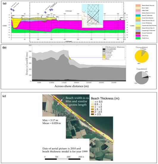
Figure 11.
Beach thickness at Happisburgh; (a) lithological model along a cross-section (section location shown as a thicker black line on small region map) showing the cliff and shore platform lithology; (b) combined profile elevation and percentage of different sediment sizes on consolidate and non-consolidated layers across a sub-domain of the lithological cross-section (sub-domain extension is indicated in panel (a) with a dashed rectangle). Total percentages of different sediment fractions shown as pie charts; (c) beach thickness along the Happisburgh coast.
4.3. Landscape Evolution Model Results
4.3.1. Model Calibration and Validation
In this work, we are interested in estimating the relative contribution of platform downwearing relative to cliff back wearing soon after the defence removal at Happisburgh. We are constrained by topographical data to start the simulation in year 1999 (i.e., the nearest date of LiDAR data to that of coastal defence removal). The failure and subsequent removal of a large part of the timber palisade defences at Happisburgh in the 1990s resulted in a 50 m cliff retreat over a 3-year period from 1996 to 1999 [34]. Annual LiDAR surveys between 2001 to 2005 showed that where the defences have failed and were removed, and where the cliffs are exposed, recession rates range from 8 to 9 m/yr [11]. For these two periods, the observed recession rates for the unprotected cliff varies from 16 m/yr (1996 to 1999) to 8 m/yr (2001 to 2005). For this exploratory work, we have assumed that for the period 1999 to 2000 the erosion rate was of the order of 12 m/yr and was spatially homogeneous along the unprotected coastal section. Calibration of the CoastalME composition used to simulate the landscape evolution requires careful consideration of: (1) the data available to calibrate the different modules; and (2) the interdependencies between the wave propagation module (CSHORE), beach and platform interaction module (SCAPE) and the alongshore sediment transport module (COVE). Table 2 shows the key calibration parameters and key model inputs used in this work.
Table 2.
CoastalME composition model inputs.
We used the UKCP09 downscaled hindcast data at 2.5 km offshore at 20 m depth to simulate the observed erosion between 1999 and 2000. The coordinates (degrees) of the downscaled wave data are: lat = 52.83 lon = 1.583. The simulation starts on 1 January 1999 00:00:00 with a 1 h time step interval. Tide data recorded at Cromer tide station every 15 min was used to reconstruct a 1 h time step tide time series starting at the same time as the wave time series. Using the harmonic coefficient obtained from the tide series spanning 18 years (1999 to 2017) at Cromer we have reconstructed the tidal elevation time series for 1999. We carried out the harmonic analysis and time series reconstruction using the UTide matlab toolbox [35]. Figure 12 shows the offshore wave forcing (significant wave height, direction and period) and the tide level. The residual elevation (e.g., the difference between the register elevation and the tidal elevation) was also calculated for 1999 (Figure A2) but not used for this simulation. The observed elevation data gap for the Cromer tide series between 17 October 1999 00:30 and 10 November 1999 13:45 was filled assuming that the residuals for this period follows a normal distribution and assuming that the mean and standard deviation are equal to the estimated residuals before filling in the gap (Figure A2).
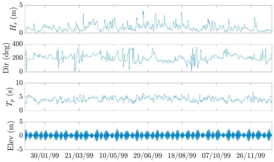
Figure 12.
Offshore wave and tidal elevation time series used as boundary conditions. The wave data is from the UKCP09 downscaled data at a point located 2.5 km offshore and 20 m depth of the study site. The elevation data are from the Cromer tide gauge station and referred to m above Newlyn datum.
The coarse, sand and fine sediment content are obtained from the 3D thickness model derived from the lithological model of the study area. In addition to differing sediment size fractions, the concept of availability factor represented within CoastalME, since erosion rates are managed separately for the different sediment fractions, in order to capture the interaction between the different sediment size fractions [36]. For each of the three sediment size fractions (coarse, sand and fine) the actual total erosion for each time step is calculated as the minimum of either the stock of sediment available or the product of the availability factor and the total potential erosion (see Equation (7) in [28]). This restriction is applied to ensure that fine sediments are more likely to be eroded, and in larger amounts, than the coarser sediments.
The key calibration parameter is the R value on the SCAPE-rock profile erosion module (see Equation (1) in [32]), representing rock strength and hydrodynamic constants (units m9/4s2/3) (i.e., an increase in R linearly decreases the amount of back-wearing and down-wearing for a given wave forcing). The R value is found by comparing model predictions of cliff recession to observations [37]. The SCAPE simulated recession rates around Happisburgh area were found to be insensitive to a two order of magnitude variation of the R-value (e.g., 0.1 R to 10 R, where R = 2 × 10⁶ m9/4s2/3) [32]. Insensitivity to R-value indicates that erosion could only occur at that location after beach material had been transported away by alongshore sediment transport, which is modulated by the CERC coefficient parameter. Variation of the CERC coefficient between 0.8 and 0.5 translates into SCAPE-simulated recession rates of 0.5 m/yr to 0.4 m/yr respectively (see Figure 16 in [32]). The SCAPE model, with these R and CERC coefficient values, is able to reproduce the observed erosion rates for a large extent of the North Norfolk and under different epochs [32]. These R and CERC coefficient values are considered here only as order of magnitude values because the assumed beach volumes were non-reported by [32] and because the observations used to validate the model [38] did not cover the Happisburgh area. Our 3D subsurface model suggest that beach thickness is minimum in front of the undefended coastline and about 0.5 m or less (see Figure 11). In SCAPE it is assumed that the beach offers full protection against platform lowering if the thickness is larger than 0.23 × Hb, where Hb is the wave height at breaking. At the study area, wave height at breaking are of the order of 1 m (i.e., that platform erosion where beach thickness is lower than 0.23 m will be non-protected). Because the beach thickness in front of the undefended coast is not thick enough to offer full protection, the R-value seems more critical than the CERC coefficient. In this context, we have used the CERC coefficient of 0.79 and independently calibrated the R-value for back wearing and downwearing as indicated below.
In addition to the resistance of the material, back wearing rate depends on the energy reaching the cliff toe and the platform downwearing is controlled by the wave energy at breaking. By using the CSHORE hydrodynamic model instead of linear theory as in SCAPE, both the wave energy at breaking and the energy reaching the cliff toe are likely to be different (i.e., in CSHORE energy dissipation due to bottom friction is non negligible while in SCAPE it is assumed negligible). This implies that to achieve the same cliff and platform erosion for a given offshore incident wave energy the R values will be different for SCAPE run within CoastalME framework, compared with SCAPE run as a standalone model. In particular, R-values will be smaller (i.e., erodibility will be larger) for SCAPE run within the CoastalME framework compared with SCAPE standalone. The magnitude of the differences on the R-values will depend on the actual bathymetry and the assumed energy dissipation due to bottom friction in CSHORE. The energy dissipation due to bottom friction in CSHORE is proportional to the product of the depth averaged cross-shore velocity and long-shore velocity (see Equation (13) in [30]). The dissipation is modulated by the non-dimensional bottom friction factor, fb, which should be calibrated using long-shore current data because of the sensitivity of long-shore currents to fb [30]. For this exploratory work (i.e., we do not have data for along-shore wave velocity) we have used the bottom friction factor of the order of 0.015 estimated for regular waves shoaling and spilling on a rough impermeable 1/35 (vertical/horizontal) slope [30]. In SCAPE, the wave height at breaking is calculated by propagating the offshore waves using linear wave theory until the wave height to depth ratio becomes equal or larger than the breaker ratio parameter, γ, which is typically in the range of γ = 0.5–1.0. In CSHORE, the cross-shore energy balance equation is solved to calculate the wave height variation due to energy dissipation due to bottom friction and breaking, CSHORE also uses the breaker ratio parameter γ to assess the threshold for wave breaking. In this work we have used γ = 0.8. In SCAPE waves are treated as regular waves but in CSHORE offshore waves are irregular: wave energy is distributed within a range of wave periods and wave heights characterized by the root mean square wave height Hrms and the representative wave period, which may be taken as the spectral peak period Tp or the spectral wave period. Because in CSHORE wave energy is distributed across a range of periods and heights at every point across a profile, in CSHORE not only is wave height calculated, but also the fraction of breaking waves, 0 ≤ Q ≤ 1, where Q = 1 means that all waves are breaking and Q = 0 means that no waves are breaking. Within the CoastalME framework, the wave breaking assumed from CSHORE results to be the point where 70% (Q = 0.7) waves are breaking. To assess the effect of using CSHORE wave propagation module rather than linear wave theory on the wave energy at breaking and at the shoreline we have run the CoastalME composition using the same inputs but changing only the wave module.
Figure A1 shows the wave height at breaking along the ca. 900 m unprotected embayment. For this comparison we have assumed an offshore wave height of Hs = 1 m, Tp = 5 s and 245° propagation angle relative to the north and spring high tide levels (+2.83 m above Mean Still Level). As expected, the wave height at breaking calculated using the CSHORE wave propagation module is significantly smaller (37% on average) than the one calculated using linear wave theory. The estimated wave height at breaking is uniform alongshore with maximum and minimum ratio of CSHORE Vs. linear wave height at breaking of 39% and 35% respectively. Assuming that, for a given offshore wave energy, the R value used in the CoastalME composition, RCoastalME, should produce similar retreat that the one computed using the R value used in the SCAPE model, RSCAPE, we can deduce that;
where F is the erosive forces under random waves in the absence of tidal variation and is equal to
the subscripts CHSORE and LINEAR indicate that the wave height at breaking, Hb, has been calculated using either CSHORE or linear theory respectively. By rearranging Equations (2) and (3) and using the average ratio of Hb calculated using CSHORE and Linear theory we obtain that;
that is, the RCSHORE value needs to be two order of magnitude smaller than the RLINEAR value to produce the same erosion for a given offshore wave energy forcing. For the platform resistance, RPlatform, we have used the above estimated value with no further calibration. For the cliff resistance, RCliff, we have tried different R values [RCliff = RPlatform, RPlatform/10, RPlatform/100] until we were able to reproduce the observed volumetric changes.
FCSHORE/RCSHORE = FLINEAR/RLINEAR
F = Hb 13/4 Tp3/2
RCSHORE = (FCSHORE/FLINEAR) x RLINEAR = (0.37)13/4 × 2∙106 m9/4s2/3 ≅ 8∙104 m9/4s2/3
4.3.2. Wave Breaking and Wave Run-Up over a Full Tidal Cycle
Figure 13 shows the cross-shore variation of the significant wave height for different water elevation along a representative transect (Figure 13a) obtained using the CSHORE hydrodynamic model. The water level has been varied from −2.23 m to +2.61 m to represent the maximum tidal range for year 1999 at Happisburgh (from Figure 12). Offshore waves conditions were Hs = 1 m, Tp = 5 s and oriented normally incident to the coast. Figure 13b shows that the waves are not affected by the bottom (i.e., appreciable change on Hs) until approximately x = 1250 m from the seaward end of the transect (i.e., approximately 1 km from the shoreline). The value of Hs at the location of 0 m profile elevation (bottom elevation = 0 in Figure 13b) varies from a maximum of 0.28 m to 0.10 m (see Table A4). Interestingly the minimum wave energy at the shore is at the maximum water level (2.61 m) and the maximum wave energy is when the water level is +2.0 m (slightly below the maximum). Figure 13c shows the fraction of wave breaking across the profile. A small percentage (<20%) breaks at the local minimum depth at the cross-shore location ca. 3000 m. The width of the surf zone (estimated as the horizontal distance between the first time that 70% of the waves are breaking to the shoreline) shows that the width is minimum (only 3 m) at minimum water level and surf-zone-width increases to 30 m at the maximum water level. The mean surf zone width for all simulated water levels is 13 m. The wave run up is calculated as 2% run up height above the location of 0 m profile elevation (bottom elevation = 0 in Figure 13d). Maximum wave run up is 3.40 m occurring at the maximum water level of 2.61 m. Simulation results show that the differences between the water level and the 2% run up increases remains fairly close to 1 m with minimum of 0.99 m and maximum of 1.09 m. On the gently sloping bottom profile near the z = 0 (slopes ~ 0.05 m/m) this implies that the cliff toe at Happisburgh can be reached without the need of additional increase on elevation due storm surges (as shown in Figure 13d).
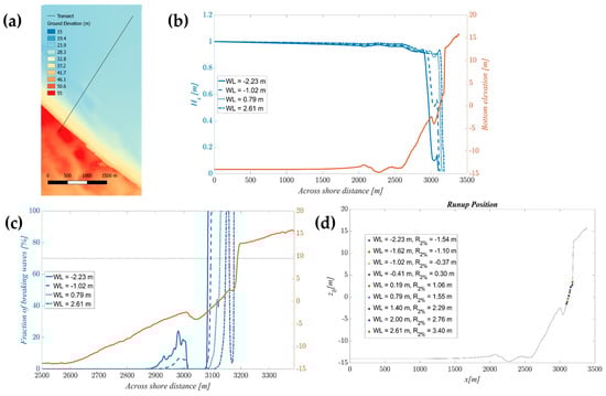
Figure 13.
CSHORE simulated wave propagation and run up along a representative Happisburgh transect; (a) location of the representative ca. 3.5 km long transect on the DEM of the study site; (b) significant wave height across-shore for different water levels along the representative transect; (c) percentage of waves breaking along the transect (the threshold of 70% used to estimate the surf zone width is represented as a dashed black line); (d) bottom profile elevation and wave run up values for each water level. The coloured circles represent the run up elevation intersection with the bottom profile.
Figure 14 shows how the active zone changes over a tidal cycle for the whole topography. The active zone is simply determined as those cells where the wave to depth breaker ratio threshold, γ, has been reached. Wave height at breaking controls the amount of cliff and platform erosion and the amount of alongshore sediment transport. If the waves are not breaking, there will be neither alongshore sediment transport nor platform erosion, but cliff back wearing could occur if the energy reaching the cliff toe is large enough to induce erosion. At every time step, the coastline is delineated on the DEM and a set of shoreline normal and polygons are created that will be later used to calculate the sediment balances (Figure 14b). We used shoreline normal of 800 m length, which seems long enough (see Figure 13a) to ensure that the waves at the seaward end of the normals are not affected by the bottom whilst not being so long that they reach DEM’s limits. If at least one cell is marked as active within a given polygon, the actual erosion and sediment transport are computed. Bottom change might occur on cells not marked as active if the erosion rates, which depend on the depth to wave height at breaking ratio, are not negligible. Figure 14b shows the cells marked as being in the active zone when the water level raised from −2.23 m to +2.61 m. Notice that, at the maximum water level of +2.61 m, the shoreline reaches the cliff toe (i.e., where ground elevation changes from pale yellow to red) but only at the north end of the embayment. Figure 14c shows the cells marked as active zone for all the simulated water levels zoomed at the north area of the embayment. The width between the most seaward active cells and the most landward active cells is ca. 130 m and ten times larger than the mean surf zone width indicating the importance of tidal levels in affecting the bottom changes.
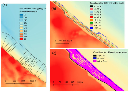
Figure 14.
Details of key modelling features over the full tidal range for the simulated year 1999; (a) shows the sediment sharing polygons that are automatically delineated at every time step. This figure shows the polygons for the shoreline delineated at the maximum water level (WL = +2.61 m); (b) delineated shoreline location at different water levels; (c) cells marked as active zones for all water levels shown in panel b. The shorelines for maximum and minimum water level are indicated for reference.
4.3.3. Daily Simulated Volumetric Changes
Table 3 shows the total accumulated platform erosion, cliff collapse, beach erosion, beach deposition and suspended sediment for the simulated year. The actual platform erosion for the study area is very close (88%) to its maximum potential erosion. This 12% reduction is due not to the limited stock of consolidated sediment but to the assumed limited availability of sand and coarse material in each time step (availability factor in Table 2). Under this assumed sediment availability, platform sediment yield is mostly dominated by fine materials with ca. 11,292 m3, followed by sand and coarse materials (70% and 30% respectively of the fine volumetric yields). The yields from cliff collapse are the largest with ca. 181,708 m3, and dominated by sands (71%), followed by fines (22%) and coarse (7%). Actual beach erosion of ca. 6,244 m3 is only 7% of the potential beach erosion as this is a sediment-limited process (i.e., alongshore sediment transport is limited by sediment availability rather than transport potential). Beach deposited is 17,376 m3, which is 2.78 times larger than the eroded beach volume, suggesting that a fraction of the sediment from the beach, and also sand and coarse material from the cliff and platform erosion are added to the beach. The difference between the total sand and coarse material eroded from the beach, cliff and platform and the deposited beach material is negative (i.e., net sediment loss from the study area) and of 141,100 m3.
Table 3.
Total accumulated annual platform erosion, cliff collapse, beach erosion, beach deposition and suspended sediment.
Figure 15 shows the accumulated beach volume changes over time. Beach volume changes (eroded and deposited) increases exponentially during the first 10 days of the simulation and more gently afterwards, disrupted only by two events of high sediment releases from platform erosion on days 203 and 264 respectively. Eroded sediment from the beach is dominated by sand, followed by coarse and fines. The dominance of sand-sized and coarse-sized sediment, despite having assumed lower availability per time step, indicates that fine material is limited on the beach at any given time. The model framework assumes that only sand and coarse materials are deposited as new beach material. Sediment added to the beach from the platform erosion ca. days 203 and 264 is clearly visible as step increases on otherwise gently sloping positive deposition time series. The amount of sediment deposited on the beach is only a small fraction of the total sediment added to the system from a combination of beach, cliff and platform erosion.
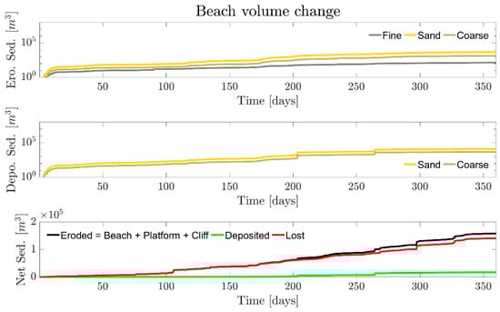
Figure 15.
Simulated beach volume accumulated changes. From top to bottom; eroded, deposited and net total sediment volume.
Figure 16 shows the daily-accumulated platform and cliff erosion during the simulated year. Accumulated eroded volumes (platform and cliff) increases exponentially during the first 10 days of the simulation and more gently afterwards, disrupted only by two events of high sediment releases of 4119 m3 and 7365 m3 from platform erosion on days 203 and 264 respectively. Note that these two single events are of a similar order of magnitude to the annually accumulated total of beach erosion. Sediment yields from the cliff are one order of magnitude larger than sediment yields from the eroding platform. Platform sediment yields are dominated by fine material, followed by sand and coarse fractions while cliff sediment yields are dominated by sand fractions followed by fine and coarse fractions.
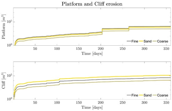
Figure 16.
Daily accumulated platform and cliff erosion sediment volume. All fine material eroded from the platform, cliff and beach becomes suspended sediment.
4.3.4. Digital Elevation Model of Topographic and Thickness Difference
Table 4 summarizes the total, beach, platform and suspended sediment volumetric changes calculated from the differences between the initial thickness model and the simulated final one. The initial total volume of 392 M m3 is mostly (99.9%) made of consolidated material with a minimum contribution of unconsolidated material. After one year of wave and tidal forcing, there is a net loss of volume of 252,343 m3 which represent less than 0.1% of the initial total sediment volume of the study area. There is also a net loss of beach volume of 112,419 m3 which represents 33% of the initial beach volume. Initial suspended sediment is zero, it increases to 52,072 m3 at the end of simulation.
Table 4.
Initial and simulated changes of sediment volumes; total, beach and platform.
Figure 17 shows the initial, final and digital elevation difference of beach thickness for different RPlatform and RCliff values. The initial beach (Figure 17a) has a maximum thickness of 3.2 m and is consistently thicker in the northern side of the embayment where the palisade and groins still in place (Figure 17b), beach thickness is a minimum in front of the embayment and is also thin at the southern side of the embayment in front of the sea wall (Figure 17c). The final beach thickness for all simulated [RPlatform, RCliff] values is on average smaller than the initial (i.e., there is a net loss of beach sediment) (Figure 17d–f). As the RCliff value decreases (i.e., cliff erodibility increases) net beach losses increases. In all cases, the beach volume is lost from the northern end of the embayment to the southern end of the seawall (Figure 17g–i) while the beach thickness on the northern side remains roughly unchanged.
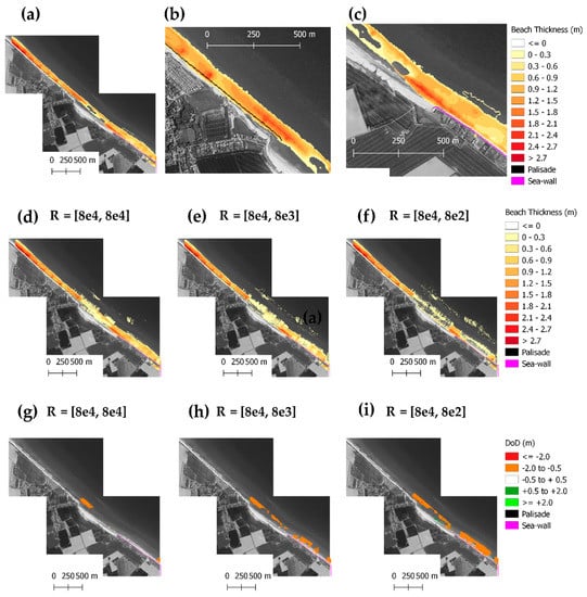
Figure 17.
Initial and final simulated beach thickness; (a) initial beach thickness derived from the lithological model; (b,c) details of the palisade in the northern side of the embayment and seawall on the southern side of the embayment respectively; (d–f) shows final beach thickness for different R values (indicated as [RPlatform, RCliff] (m9/4s2/3)); (g–i) shows the thickness difference between the final and initial beach thickness.
Figure 18 shows the final and digital elevation difference of platform elevation for different RPlatform and RCliff values. For the simulated cases where RCliff = RPlatform and RPlatform/10, the changes on platform elevation are non-appreciable (i.e., change less than 0.5 m). For the smallest RCliff = RPlatform/100 value, platform erosion is significant (i.e., changes larger than 0.5 m) in the embayment area and insignificant elsewhere. Some erosion at the cliff toe behind the palisade is also appreciable for the simulated case with maximum cliff erodibility.
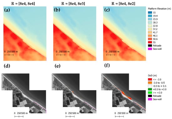
Figure 18.
Simulated final and net platform-elevation change; (a–c) final simulated platform elevation for different R-values (indicated as [RPlatform, RCliff] (m9/4s2/3)); (d–f) shows the digital elevation differences of platform elevation between the final and initial values.
5. Discussion
5.1. Happisburgh Beach Conceptualized as a Thin but Non-Sediment Starving Beach
In this work we have provided a range of evidence to support the idea that the Happisburgh beach is a thin layer perched on a sediment rich platform of sand and gravel. This conceptualization differs from [3], which assumes that the platform was mostly till and fine material. We have shown here that while till might be relatively abundant on the emerged cliff, the mostly sand and gravel Crag Group dominates the lithology of the submerged platform (Figure 8). We have also shown, for first time, how the beach thickness varies along the study area from a maximum of 3.7 m to almost zero in the embayment area (Figure 11). The combined effects of the platform being rich in potential beach material, and beach thickness along the embayment being less than that necessary to provide protection have been explored numerically using the CoastalME framework [28]. Our annual simulations (Figure 17f,i) show that net beach volume decreases by about 33% of its initial volume at an annual rate of 141,100 m3/yr, consistent with the reported average annual losses of 150,000 m3/yr [6]. The beach volume is mostly lost from the embayment region and the area in front of the seawall, while it remains mostly unchanged on the northern side of the study area. Our simulations also show that a platform lowering of the order of 1 to 2 m occurs along the embayment region where beach thickness is initially a minimum. Interestingly, simulations show no platform lowering on the northern region, where the palisade and groins are still in place, and beach thicknesses are greatest. The passive seismic survey results, conducted at the northern side of the embayment, were inconclusive regarding the presence of a step elevation change in front of the palisade as the Crag Group has similar impedance to the contemporaneous beach (Figure 10). Nevertheless, the passive seismic analysis provides reassurance that the chalk surface is too deep to be affected by the wave action on an annual time scale.
5.2. Contribution of Platform Back-Wearing and Down-Wearing to Near-Shore Sediment Budgets
We found that the cliff sediment yield is ten times larger than the platform sediment yield, but sediment from platform erosion is of a similar order of magnitude to the eroded beach material, and is therefore important to close the sediment budget (Table 2). Cliff collapse yields 181,708 m3 in one year, and is mostly sand and gravel (71% and 7% respectively) while platform erosion yields 11,292 m3 in one year of sand and gravel. The total accumulated deposited material on the beach is 17,376 m3/yr. Not including the sediment yields from platform erosion will translate into non-including 64% of the deposited beach material.
Most (141,100 m3/yr) of the sediment yield from cliff and platform erosion is lost from the grid due to alongshore sediment transport (assumed open boundary conditions, Table 2). It is not possible to quantify how much of the material is deposited from the sediment eroded from the cliff and the platform.
5.3. Implications and Limitations
The main implications of the findings of this work concern the future expected evolution of the Happisburgh coastline and the safety standard of the existing defences. We could not find any field or numerical evidence of platform lowering in front of the palisade at the northern region of the embayment. The lack of field evidence is most likely related to the lack of impedance contrast across the local lithologies. The lack of numerical evidence of platform lowering at the northern region suggests that, when defences are in place, the beach is thick enough to protect the underlying platform. Numerical evidence nevertheless suggests that the embayment will continue developing due to the removal of beach material from the northern end of the embayment. The estimated lowering in front of the seawall at the southern end, combined with the decrease on the beach volume implies that depth at the toe of the sea wall is increasing, allowing larger waves to reach the toe and therefore, increasing the risk of sea wall failure.
We need to acknowledge a number of limitations of this study and the results presented here. The lack of quantitative data on rates of platform lowering imposes serious limitations for the simulations of landscape evolution. Platform resistance was calibrated by building on reported values in the literature and some reasoning around how the hydrodynamic forcing might differ from the one used on the reported values. Ideally, we would have calibrated this bulk resistance value by matching observed platform lowering data. The cliff resistance value was calibrated but not fine-tuned using existing LiDAR data; rather an order of magnitude approach was followed. The lack of bathymetric data for the shallow nears-hore also introduces uncertainties in the simulations of landscape evolution. Our simulation results for hydrodynamic wave propagation under different water levels show that small elevation changes have important effects on the wave energy at breaking and the energy reaching the cliff toe. We have not used a meteorological surges time series in the simulations because the maximum water levels were smaller after meteorological surge was added to the tidal time series. A more detailed sensitivity analysis of the effect of R values, bathymetry, and water levels was not feasible for this exploratory work but it will be needed to assess the relative error of each element.
6. Conclusions
This study examined beach thickness and geologic framework control on the cliff and platform erosion after coastal defence removal at Happisburgh, UK. For the first time we have shown that, the beach thickness at the study site is non-uniform alongshore and that the consolidated platform sediment is rich in sand and gravel fractions and therefore an important potential source of material for the beach. We used the Coastal Modelling Environment framework to assess the relative contribution of back wearing and down wearing cliff and platform erosion to the near-shore sediment budget under idealized forcing conditions. The results suggest that the often-neglected down wearing contribution is of a similar order of magnitude to the beach volume losses and therefore non-negligible. Further work is required to determine the contribution of down wearing sediment yields to the near-shore sediment budget. The present effort contributes to our understanding of coastal sediment budgeting and outlines a quantitative approach that will allow for simple integration of geological understanding on coastlines evolution assessments worldwide.
Supplementary Materials
The CoastalME software version, including all the input files used in this study, can be found here: https://doi.org/10.5281/zenodo.1418854.
Author Contributions
Conceptualization, A.P. and M.W.; Methodology, A.P.; Software-CoastalME, D.F.-M. and A.P.; Software-GroundHog B.W., H.B. and H.K.; Validation, A.P. and M.W.; Formal Analysis, A.P.; Investigation, A.P., M.W., J.L.; Resources, M.A.E.; Data Collection, A.P., A.B., H.B.; Writing—Original Draft Preparation, A.P.; Writing—Review & Editing, A.B. and M.E; Visualization, A.P. and B.W.; Project Administration, A.P. and M.A.E.; Funding Acquisition, M.A.E.
Funding
This research was funded by the UK Natural Environment Research Council (NE/M004996/1; BLUE-coast project). Collaboration with Mike Walkden, from WSP Group was possible thanks to British Geological Survey Innovation Flexible Funds.
Acknowledgments
Thank you to all those who assisted with the preparation of this manuscript, in particular Brad Johnson from the Army Corp of Engineers (USA) and Nobuhisa Kobayashi for their support with the CSHORE model. Additional data were provided by United Kingdom Hydrographic Office (UKHO), the Environment Agency (EA) and the British Oceanographic Centre (BODC), containing public sector information licensed under the Open Government License v3.0.
Conflicts of Interest
The authors declare no conflict of interest.
Appendix A. Criteria for Reliable and Clear H/V
This appendix contains the criteria for reliable H/V curve and H/V peak according to the SESAME, guidelines [22] implemented in the Grilla software, for the observations at the seaward and landward side of the palisade.
Table A1.
Reliability of H/V curve and clarity of H/V peak recorded at the seaward side of the palisade.
| Max. H/V at 2.5 ± 54.26 Hz (in the Range 0.0–512.0 Hz). | |||
|---|---|---|---|
| Criteria for a reliable H/V curve [All 3 should be fulfilled] | |||
| f0 > 10/Lw | 2.50 > 2.00 | OK | |
| nc(f0) > 200 | 512.5 > 200 | OK | |
| sA(f) < 2 for 0.5f0 < f < 2f0 if f0 > 0.5Hz | Exceeded 0 out of 31 times | OK | |
| sA(f) < 3 for 0.5f0 < f < 2f0 if f0 < 0.5Hz | |||
| Criteria for a clear H/V peak [At least 5 out of 6 should be fulfilled] | |||
| Exists f− in [f0/4, f0] | AH/V(f−) < A0/2 | 1.5 Hz | OK | |
| Exists f+ in [f0, 4f0] | AH/V(f+) < A0/2 | 5.5 Hz | OK | |
| A0 > 2 | 4.20 > 2 | OK | |
| fpeak[AH/V(f) ± sA(f)] = f0 ± 5% | |21.70298| < 0.05 | NO | |
| sf < e(f0) | 54.25745 < 0.125 | NO | |
| sA(f0) < q(f0) | 1.2164 < 1.58 | OK | |
| Threshold Values for sf and sA(f0) | |||||
|---|---|---|---|---|---|
| Freq. range [Hz] | <0.2 | 0.2–0.5 | 0.5–1.0 | 1.0–2.0 | >2.0 |
| e(f0) [Hz] | 0.25 f0 | 0.2 f0 | 0.15 f0 | 0.10 f0 | 0.05 f0 |
| q(f0) for sA(f0) | 3.0 | 2.5 | 2.0 | 1.78 | 1.58 |
| log q(f0) for slogH/V(f0) | 0.48 | 0.40 | 0.30 | 0.25 | 0.20 |
Table A2.
Reliability of H/V curve and clarity of H/V peak recorded at the landward side of the palisade.
| Max. H/V at 2.75 ± 0.92 Hz (in the Range 0.0–512.0 Hz). | |||
|---|---|---|---|
| Criteria for a reliable H/V curve [All 3 should be fulfilled] | |||
| f0 > 10/Lw | 2.75 > 2.00 | OK | |
| nc(f0) > 200 | 495.0 > 200 | OK | |
| sA(f) < 2 for 0.5f0 < f < 2f0 if f0 > 0.5Hz | Exceeded 0 out of 34 times | OK | |
| sA(f) < 3 for 0.5f0 < f < 2f0 if f0 < 0.5Hz | |||
| Criteria for a clear H/V peak [At least 5 out of 6 should be fulfilled] | |||
| Exists f− in [f0/4, f0] | AH/V(f −) < A0/2 | 1.5 Hz | OK | |
| Exists f+ in [f0, 4f0] | AH/V(f +) < A0/2 | 5.125 Hz | OK | |
| A0 > 2 | 3.98 > 2 | OK | |
| fpeak[AH/V(f) ± sA(f)] = f0 ± 5% | |0.33445| < 0.05 | NO | |
| sf < e(f0) | 0.91974 < 0.1375 | NO | |
| sA(f0) < q(f0) | 1.2647 < 1.58 | OK | |
| Lw | window length |
| nw | number of windows used in the analysis |
| nc = Lw nw f0 | number of significant cycles |
| f | current frequency |
| f0 | H/V peak frequency |
| sf | standard deviation of H/V peak frequency |
| e(f0) | threshold value for the stability condition sf < e(f0) |
| A0 | H/V peak amplitude at frequency f0 |
| AH/V(f) | H/V curve amplitude at frequency f |
| f− | frequency between f0/4 and f0 for which AH/V(f−) < A0/2 |
| f+ | frequency between f0 and 4f0 for which AH/V(f+) < A0/ |
| sA(f) | standard deviation of AH/V(f), sA(f) is the factor by which the mean AH/V(f) curve should be multiplied or divided |
| slogH/V(f) | standard deviation of log AH/V(f) curve |
| q(f0) | threshold value for the stability condition sA(f) < q(f0) |
| Threshold Values for sf and sA(f0) | |||||
|---|---|---|---|---|---|
| Freq. range [Hz] | <0.2 | 0.2–0.5 | 0.5–1.0 | 1.0–2.0 | >2.0 |
| e(f0) [Hz] | 0.25 f0 | 0.2 f0 | 0.15 f0 | 0.10 f0 | 0.05 f0 |
| q(f0) for sA(f0) | 3.0 | 2.5 | 2.0 | 1.78 | 1.58 |
| log q(f0) for slogH/V(f0) | 0.48 | 0.40 | 0.30 | 0.25 | 0.20 |
Appendix B. Supplementary Lithological, Hydrodynamic and Morphodynamic Information
Table A3.
Assigned average percentages for fines (<0.63 mm), sand (0.63–2 mm) and coarse material (>2 mm) for the different lithostratigraphical units expressed in the 3D subsurface model.
Table A3.
Assigned average percentages for fines (<0.63 mm), sand (0.63–2 mm) and coarse material (>2 mm) for the different lithostratigraphical units expressed in the 3D subsurface model.
| Name | Lithology | Coarse [%] | Sand [%] | Fine [%] |
|---|---|---|---|---|
| Marine beach deposits | Shoreline sand and gravel | 10 | 89 | 1 |
| Coastal barrier deposits | sand and gravel | 10 | 89 | 1 |
| Breydon Formation | Holocene peat, silt, clay. Tidal alluvium | 2 | 30 | 68 |
| Blown sand | wind blown sand | 0.5 | 84.5 | 15 |
| Valley head | clay, silt, sand, gravel | 10 | 35 | 55 |
| Aldeby Sand and Gravel | Sand and gravel overlying chalky till | 10 | 83 | 7 |
| Walcott Till Member | Very chalky till, up to 70 per cent | 15 | 7.5 | 77.5 |
| Corton Sand Member | sand, with some gravel | 5 | 85 | 10 |
| Glacial silt and clay | laminated silt and clay (mud) | 0.5 | 10 | 89.5 |
| Corton Till Member | Sandy, silty diamicton (aka brickearth) | 10 | 35 | 55 |
| Happisburgh Sand Member | Sand | 2 | 90 | 8 |
| Glacial silt and clay | laminated silt and clay (mud) | 0.5 | 10 | 89.5 |
| Happisburgh Till Member | Sandy, silty diamicton | 10 | 35 | 55 |
| Cromer Forest-bed | mud | 10 | 30 | 60 |
| Crag Group | sand | 5 | 85 | 10 |
| chalk | chalk | 15 | 2 | 83 |

Figure A1.
Calculated wave height at breaking, Hb, along the undefended coastline using CSHORE propagation module and linear wave theory as in the COVE model. The northern end refers to the limit of the un-defended coastline.
Figure A1.
Calculated wave height at breaking, Hb, along the undefended coastline using CSHORE propagation module and linear wave theory as in the COVE model. The northern end refers to the limit of the un-defended coastline.

Table A4.
Water levels, significant wave height at the shore (z = 0) and 2% run up above z = 0 CSHORE simulated results along the transect shown in Figure 13c and assuming offshore waves Hs = 1 m, Tp = 5 s, and normal to the coast incident angle.
Table A4.
Water levels, significant wave height at the shore (z = 0) and 2% run up above z = 0 CSHORE simulated results along the transect shown in Figure 13c and assuming offshore waves Hs = 1 m, Tp = 5 s, and normal to the coast incident angle.
| Water Level (m) | Hs at z = 0 (m) | 2% Run Up |
|---|---|---|
| −2.23 | 0.13 | −1.54 |
| −1.62 | 0.16 | −1.10 |
| −1.02 | 0.16 | −0.37 |
| −0.41 | 0.23 | 0.30 |
| 0.19 | 0.19 | 1.06 |
| 0.79 | 0.20 | 1.55 |
| 1.40 | 0.24 | 2.29 |
| 2.00 | 0.28 | 2.76 |
| 2.61 | 0.10 | 3.40 |

Figure A2.
Offshore residual surge elevation time series. The elevation data are from the Cromer tide gauge station and referred to m above Newlyn datum. The data gap on the Elevation data is shown on the residual elevation plot as black line.
Figure A2.
Offshore residual surge elevation time series. The elevation data are from the Cromer tide gauge station and referred to m above Newlyn datum. The data gap on the Elevation data is shown on the residual elevation plot as black line.

References
- Pontee, N.I.; Parsons, A. A review of coastal risk management in the UK. Proc. Inst. Civ. Eng.-Marit. Eng. 2010, 163, 31–42. [Google Scholar] [CrossRef]
- Dickson, M.E.; Walkden, M.J.A.; Hall, J.W. Systemic impacts of climate change on an eroding coastal region over the twenty-first century. Clim. Chang. 2007, 84, 141–166. [Google Scholar] [CrossRef]
- Walkden, M.; Watson, G.; Johnson, A.; Heron, E.; Tarrant, O. Coastal catch-up following defence removal at Happisburgh. In Coastal Management; ICE Publishing: London, UK, 2016; pp. 523–532. [Google Scholar]
- Payo, A.; Walkden, M.; Barkwith, A.; Ellis, A.M. Modelling rapid coastal catch-up after defence removal along the soft cliff coast of Happisburgh, UK. In Proceedings of the 36th International Conference on Coastal Engineering, Baltimore, MD, USA, 30 July–3 August 2018; ASCE: Baltimore, MD, USA; p. 2. [Google Scholar]
- Shennan, I.; Woodworth, P.L. A comparison of late holocene and twentieth-century sea-level trends from the UK and North Sea region. Geophys. J. Int. 1992, 109, 96–105. [Google Scholar] [CrossRef]
- Hayman, S. Eccles to Winterton on Sea Coastal Defences; SH/RG BF190712; Environment Agency: Bristol, UK, 2012; p. 3. [Google Scholar]
- Wolf, J.; Lowe, J.; Howard, T. Climate downscaling: Local mean sea level, surge and wave modelling. In Broad Scale Coastal Simulation; Springer: Berlin, Germany, 2015; pp. 79–102. [Google Scholar]
- Geos, F. Wind and Wave Frequency Distributions for Sites around the British Isles; Health and Safety Executive: Bootle, UK, 2001. [Google Scholar]
- Brown, S.; Barton, M.E.; Nicholls, R.J. Shoreline response of eroding soft cliffs due to hard defences. Proc. ICE-Marit. Eng. 2014, 167, 3–14. [Google Scholar]
- Clayton, K.M. Sediment input from the norfolk cliffs, eastern england—A century of coast protection and its effect. J. Coast. Res. 1989, 5, 433–442. [Google Scholar]
- Poulton, C.V.; Lee, J.; Hobbs, P.; Jones, L.; Hall, M. Preliminary investigation into monitoring coastal erosion using terrestrial laser scanning: Case study at Happisburgh, Norfolk. Bull. Geol. Soc. Norfolk 2006, 56, 45–64. [Google Scholar]
- Frew, P. Adapting to coastal change in north Norfolk, UK. Proc. Inst. Civ. Eng.-Marit. Eng. 2012, 165, 131–138. [Google Scholar] [CrossRef]
- Lunkka, J.P. Sedimentation and iithostratigraphy of the north sea drift and lowestoft till formations in the coastal cliffs of northeast Norfolk, England. J. Quat. Sci. 1994, 9, 209–233. [Google Scholar] [CrossRef]
- Lee, J.R. Early and Middle Pleistocene Lithostratigraphy and Palaeo-Environments in Northern East Anglia; Royal Holloway, University of London: London, UK, 2003. [Google Scholar]
- Lee, J.R.; Phillips, E.R. Progressive soft sediment deformation within a subglacial shear zone—A hybrid mosaic-pervasive deformation model for middle pleistocene glaciotectonised sediments from eastern England. Quat. Sci. Rev. 2008, 27, 1350–1362. [Google Scholar] [CrossRef]
- Lee, J.R.; Phillips, E.; Rose, J.; Vaughan-Hirsch, D. The middle pleistocene glacial evolution of northern East Anglia, UK: A dynamic tectonostratigraphic–parasequence approach. J. Quat. Sci. 2017, 32, 231–260. [Google Scholar] [CrossRef]
- Parfitt, S.A.; Ashton, N.M.; Lewis, S.G.; Abel, R.L.; Coope, G.R.; Field, M.H.; Gale, R.; Hoare, P.G.; Larkin, N.R.; Lewis, M.D. Early pleistocene human occupation at the edge of the boreal zone in northwest europe. Nature 2010, 466, 229–233. [Google Scholar] [CrossRef] [PubMed]
- West, R.G. The Pre-Glacial Pleistocene of the Norfolk and Suffolk Coasts. Archeol. J. 1981, 138, 266–267. [Google Scholar]
- Aki, K.; Richards, P.G. Quantitative Seismology; University Science Books: Sausalito, CA, USA, 2002. [Google Scholar]
- Ari, B.-M.; Singh, S.J. Seismic Waves and Sources; Springer: New York, NY, USA, 1981. [Google Scholar]
- Guillier, B.; Chatelain, J.-L.; Bonnefoy-Claudet, S.; Haghshenas, E. Use of ambient noise: From spectral amplitude variability to H/V stability. J. Earthq. Eng. 2007, 11, 925–942. [Google Scholar] [CrossRef]
- SESAME. Guidelines for the Implementation of the H/V Spectral Ratio Technique on Ambient Vibrations-Measurements, Processing and Interpretation; Sesame European Research Project, Deliverable d23. 12., Project No; EVG1-CT-2000-00026 SESAME, 62; 2004; Available online: http://www.geopsy.org/ (accessed on 4 October 2018).
- Bonnefoy-Claudet, S.; Köhler, A.; Cornou, C.; Wathelet, M.; Bard, P.Y. Effects of love waves on microtremor h/v ratio. Bull. Seismol. Soc. Am. 2008, 98, 288–300. [Google Scholar] [CrossRef]
- Conrad, O.; Bechtel, B.; Bock, M.; Dietrich, H.; Fischer, E.; Gerlitz, L.; Wehberg, J.; Wichmann, V.; Böhner, J. System for automated geoscientific analyses (saga) v. 2.1.4. Geosci. Model Dev. 2015, 8, 1991–2007. [Google Scholar] [CrossRef]
- Smith, W.; Wessel, P. Gridding with continuous curvature splines in tension. Geophysics 1990, 55, 293–305. [Google Scholar] [CrossRef]
- Kessler, H.; Mathers, S.; Sobisch, H.-G. The capture and dissemination of integrated 3d geospatial knowledge at the british geological survey using gsi3d software and methodology. Comput. Geosci. 2009, 35, 1311–1321. [Google Scholar] [CrossRef]
- Payo, A.; Favis-Mortlock, D.; Dickson, M.; Hall, J.W.; Hurst, M.; Walkden, M.J.A.; Townend, I.; Ives, M.C.; Nicholls, R.J.; Ellis, M.A. Coastalme version 1.0: A coastal modelling environment for simulating decadal to centennial morphological changes. Geosci. Model Dev. Discuss. 2016, 2016, 1–45. [Google Scholar] [CrossRef]
- Payo, A.; Favis-Mortlock, D.; Dickson, M.; Hall, J.W.; Hurst, M.D.; Walkden, M.J.A.; Townend, I.; Ives, M.C.; Nicholls, R.J.; Ellis, M.A. Coastal modelling environment version 1.0: A framework for integrating landform-specific component models in order to simulate decadal to centennial morphological changes on complex coasts. Geosci. Model Dev. 2017, 10, 2715–2740. [Google Scholar] [CrossRef]
- Hurst, M.D.; Barkwith, A.; Ellis, M.A.; Thomas, C.W.; Murray, A.B. Exploring the sensitivities of crenulate bay shorelines to wave climates using a new vector-based one-line model. J. Geophys. Res. Earth Surf. 2015, 120, 2586–2608. [Google Scholar] [CrossRef]
- Kobayashi, N. Coastal sediment transport modeling for engineering applications. J. Waterw. Port Coast. Ocean Eng. 2016, 142, 03116001. [Google Scholar] [CrossRef]
- Walkden, M.; Dickson, M.; Thomas, J.; Hall, J. Probabilistic Simulation of Long Term Shore Morphology of North Norfolk UK; World Scientific: Singapore, 2009; pp. 4365–4377. [Google Scholar]
- Walkden, M.J.; Hall, J.W. A mesoscale predictive model of the evolution and management of a soft-rock coast. J. Coast. Res. 2011, 27, 529–543. [Google Scholar] [CrossRef]
- Self, S.; Entwisle, D.; Northmore, K. The Structure and Operation of the BGS National Geotechnical Properties Database; Version 2; British Geological Survey: Nottingham, UK, 2012. [Google Scholar]
- Ohl, C.; Frew, P.; Sawyers, P.; Watson, G.; Lawton, P.; Farrow, B.; Walkden, M.; Hall, J. North Norfolk—A regional approach to coastal erosion management and sustainability in practice. In Proceedings of the International Conference on Coastal ManagementInstitution of Civil Engineers 2003, Brighton, UK, 15–17 October 2003. [Google Scholar]
- Codiga, D.L. Unified Tidal Analysis and Prediction Using the Utide Matlab Functions; Graduate School of Oceanography, University of Rhode Island: Narragansett, RI, USA, 2011. [Google Scholar]
- Le Hir, P.; Cayocca, F.; Waeles, B. Dynamics of sand and mud mixtures: A multiprocess-based modelling strategy. Cont. Shelf Res. 2011, 31, S135–S149. [Google Scholar] [CrossRef]
- Walkden, M.J.A.; Hall, J.W. A predictive mesoscale model of the erosion and profile development of soft rock shores. Coast. Eng. 2005, 52, 535–563. [Google Scholar] [CrossRef]
- Cambers, G. Temporal scales in coastal erosion systems. Trans. Inst. Br. Geogr. 1976, 1, 246–256. [Google Scholar] [CrossRef]


© 2018 by the authors. Licensee MDPI, Basel, Switzerland. This article is an open access article distributed under the terms and conditions of the Creative Commons Attribution (CC BY) license (http://creativecommons.org/licenses/by/4.0/).