Author Contributions
Conceptualization, A.P. and M.W.; Methodology, A.P.; Software-CoastalME, D.F.-M. and A.P.; Software-GroundHog B.W., H.B. and H.K.; Validation, A.P. and M.W.; Formal Analysis, A.P.; Investigation, A.P., M.W., J.L.; Resources, M.A.E.; Data Collection, A.P., A.B., H.B.; Writing—Original Draft Preparation, A.P.; Writing—Review & Editing, A.B. and M.E; Visualization, A.P. and B.W.; Project Administration, A.P. and M.A.E.; Funding Acquisition, M.A.E.
Figure 1.
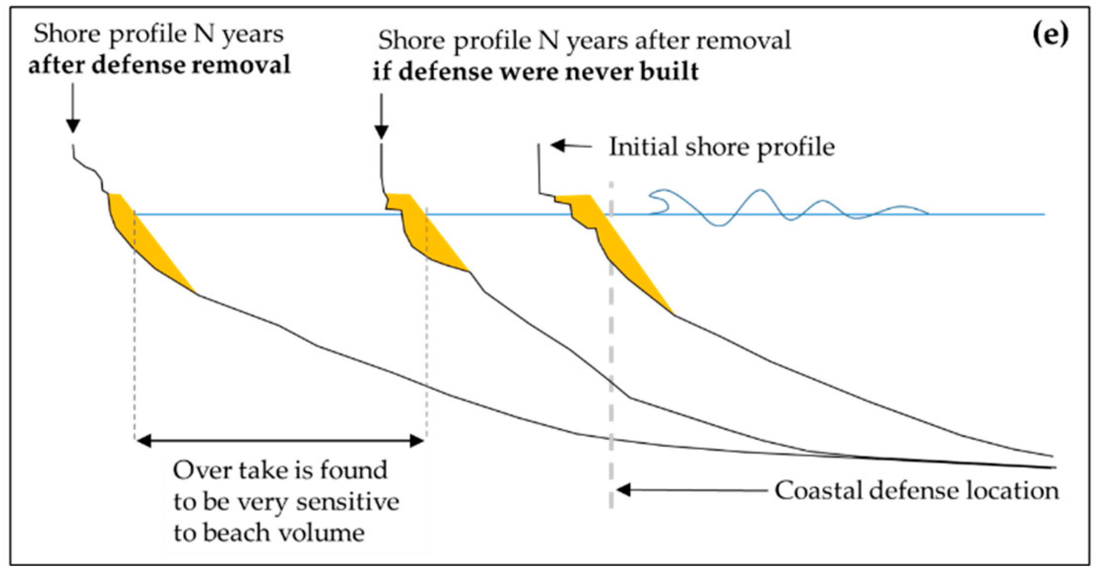
Illustration of the development and loss of a step in the shore platform profile due to the construction and removal of a vertical coast protection. Beach volume is represented as a yellow polygon and shore platform profile as a black solid line. The panels show an idealized beach and shore platform evolution; (a) initial beach and shore platform profile at the time of construction of the coastal defence; (b) after the construction of the defence, shore platform lowering (red arrows) seaward of the defence is larger than behind, and so a step develops; (c) when the defence is removed, the (steepened) shore platform previously behind the step is exposed to higher wave energy, inducing rapid shore platform and cliff retreat (the shore platform in front of the structure continues to erode at a low rate); (d) after a period of time the step is removed and a new quasi-equilibrium coupled beach and shore platform profile is reached; retreat rates then reduce and become more steady; (e) sensitivity analysis has shown that the ‘overtake’ (i.e., excess net shoreline retreat caused by this process) increases if beach volume decreases.
Figure 1.
Illustration of the development and loss of a step in the shore platform profile due to the construction and removal of a vertical coast protection. Beach volume is represented as a yellow polygon and shore platform profile as a black solid line. The panels show an idealized beach and shore platform evolution; (a) initial beach and shore platform profile at the time of construction of the coastal defence; (b) after the construction of the defence, shore platform lowering (red arrows) seaward of the defence is larger than behind, and so a step develops; (c) when the defence is removed, the (steepened) shore platform previously behind the step is exposed to higher wave energy, inducing rapid shore platform and cliff retreat (the shore platform in front of the structure continues to erode at a low rate); (d) after a period of time the step is removed and a new quasi-equilibrium coupled beach and shore platform profile is reached; retreat rates then reduce and become more steady; (e) sensitivity analysis has shown that the ‘overtake’ (i.e., excess net shoreline retreat caused by this process) increases if beach volume decreases.
![Jmse 06 00113 g001a]()
![Jmse 06 00113 g001b]()
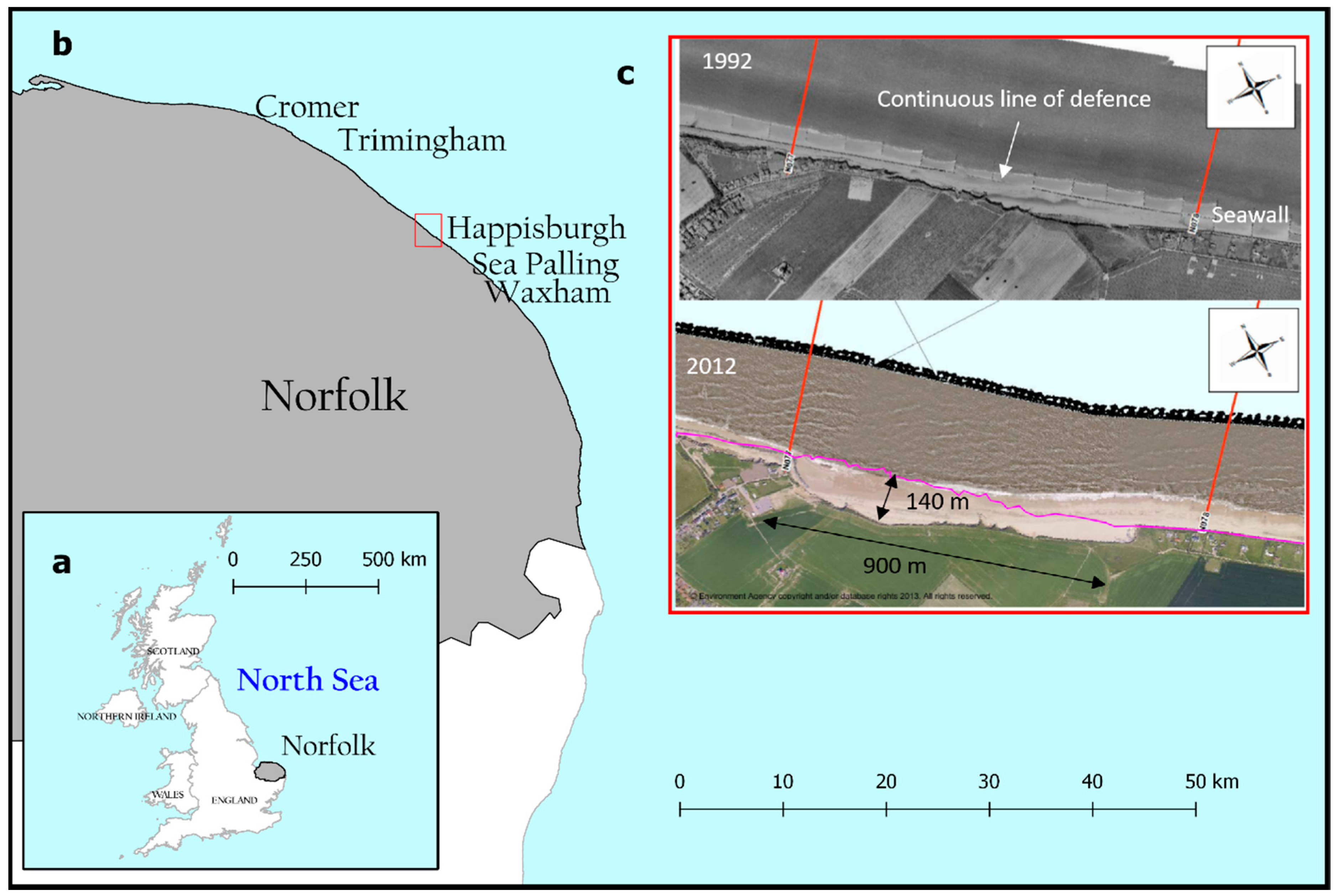
Figure 2.
Study location: (a) Happisburgh is located in county of Norfolk (grey polygon) on the east coast of England, the grey lines represent the administrative boundaries of the different UK regions; (b) study site location (red rectangle) and nearby locations mentioned on this manuscript; (c) aerial images of Happisburgh taken in 1992 and 2012 by the Environment Agency; showing the formation of an embayment. Red lines indicate the location of profile monitoring surveys, and the magenta line shows the approximate cliff toe position in 1992.
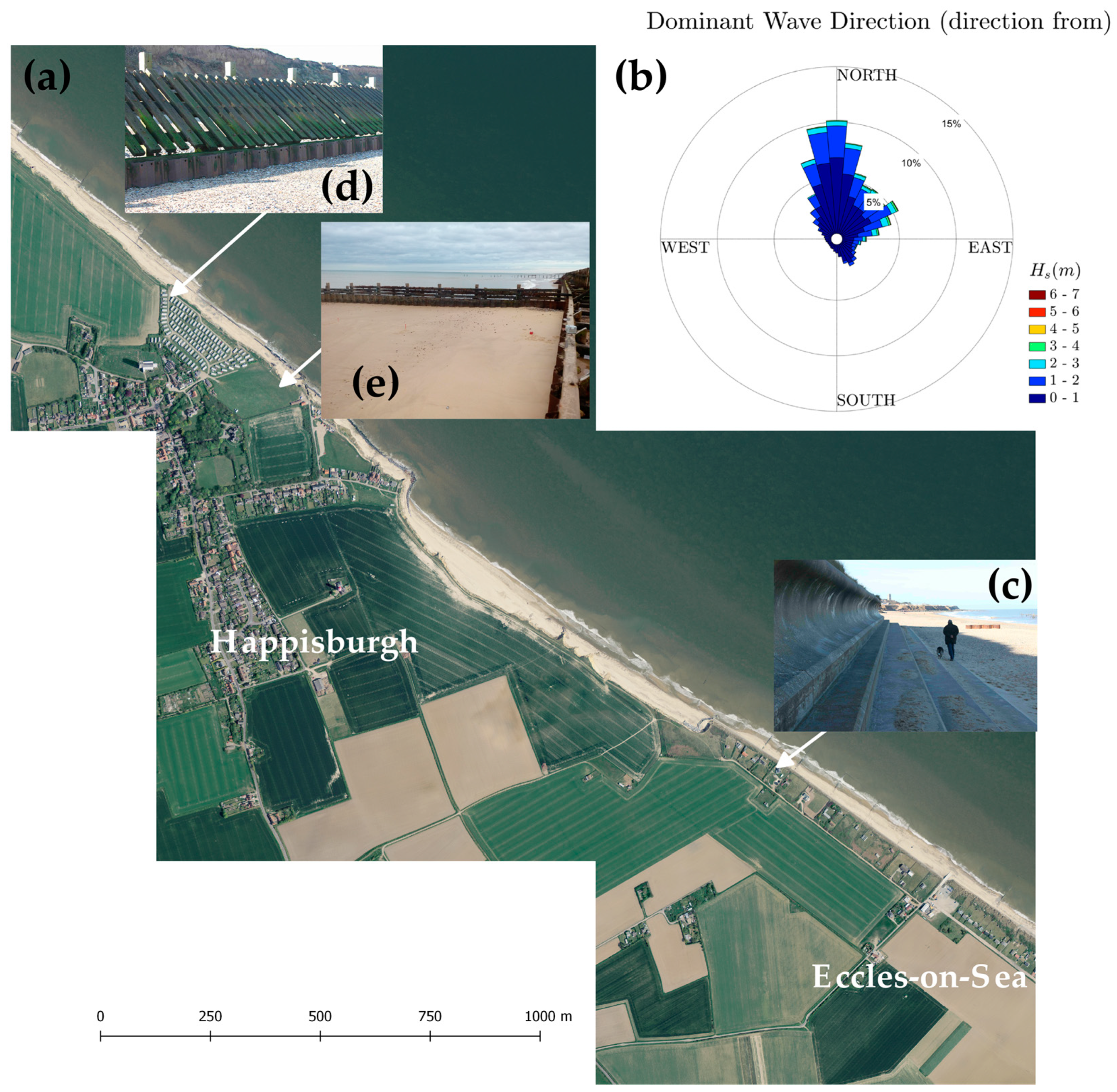
Figure 3.
Study site: (a) aerial view of the study region in 2010 showing the embayment (source EA, year 2010); (b) wave rose for Happisburgh created using downscaled data (1961–2016) from the UKCP09; (c) detail of the sea-wall protecting the low-lying coast of Eccles-on-Sea; (d) view of the wood revetment and sheet pile that is still in place northwest of Happisburgh (source Mike Walkden, year 2013); (e) detail of wooden groin used to slow down the alongshore sediment transport (source Andres Payo, 2017).
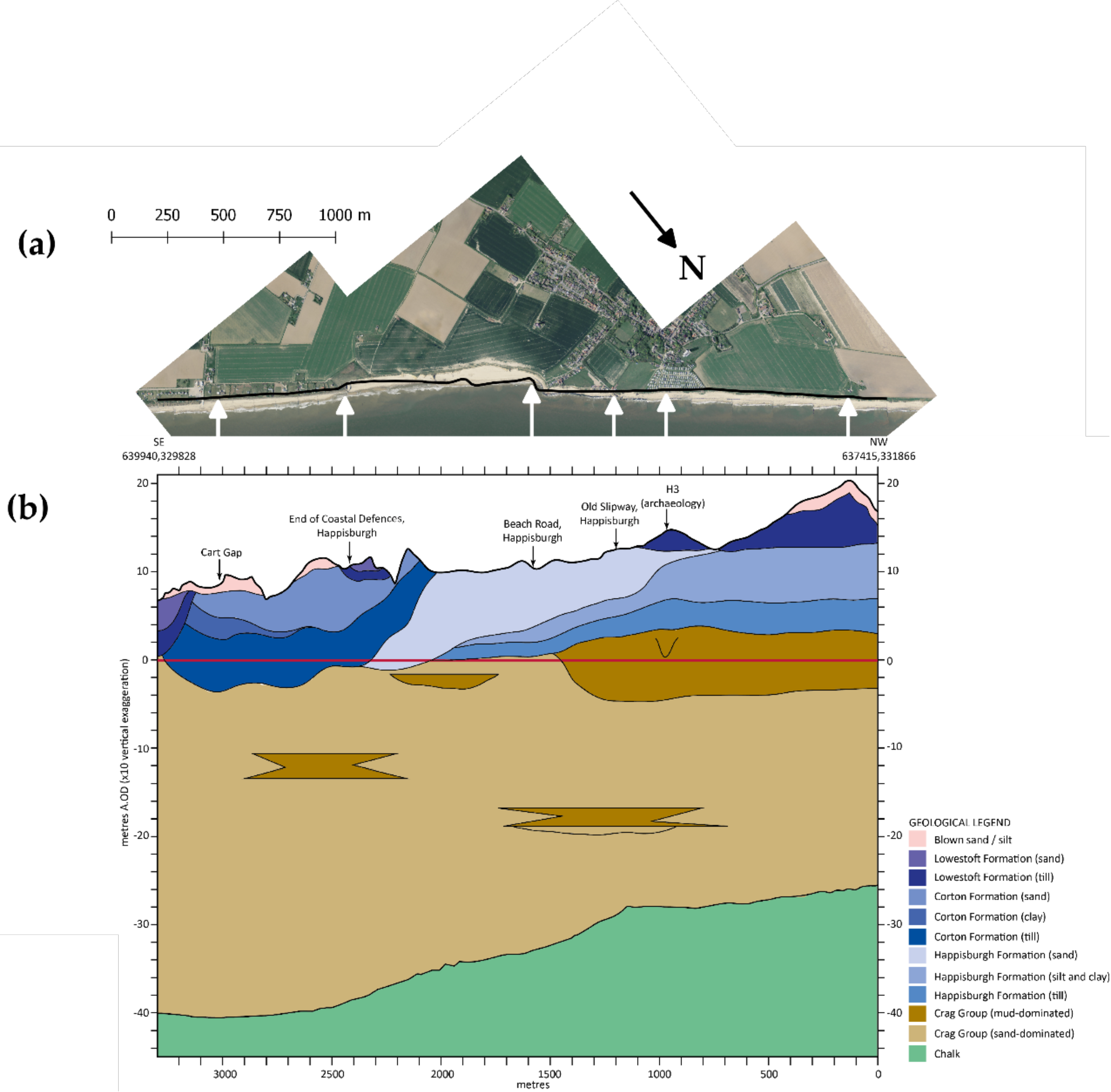
Figure 4.
Main geological units at the study site along the 1999 cliff top line: (a) cliff top line of year 1999 is shown as solid black line on top of year 2010 aerial photography of the study site; (b) main lithological units. Key landmarks along the cliff cross section are named in (b), approximate locations on (a) are indicated by white arrows. Across-shore distances are distances measured along the cliff top line (starting at the northern end) and vertical elevation are relative to Ordnance Datum (which is approximately at mean sea level for the study site). For clarity, the vertical scale has been exaggerated 10 times.
Figure 5.
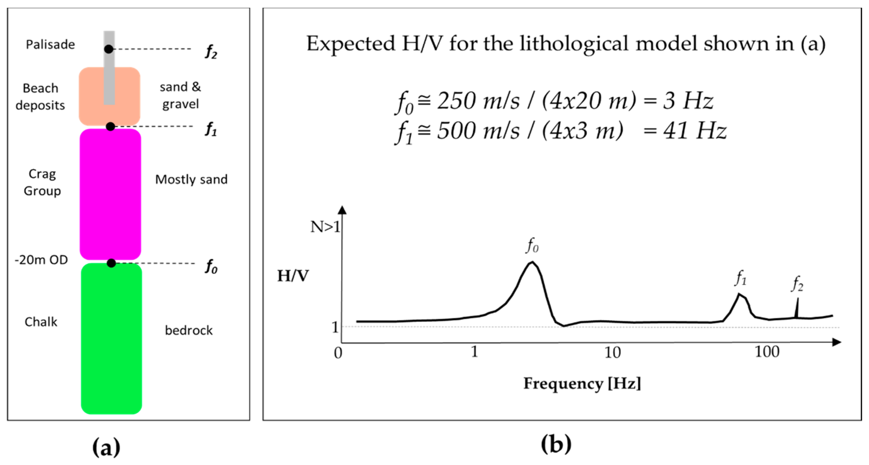
Expected spectral noise Horizontal to Vertical (H/V) ratio for the assumed lithological model on the beach at Happisburgh; (a) lithological model showing the main lithologies, their composition (i.e., sand, gravel, bedrock) and the expected peak frequencies; (b) expected H/V and approximated values of the lithological peaks f0 and f1. The f2 peak is an expected non-lithological signal (i.e., sharper than lithological peaks) resulting from the man-made coastal defence.
Figure 5.
Expected spectral noise Horizontal to Vertical (H/V) ratio for the assumed lithological model on the beach at Happisburgh; (a) lithological model showing the main lithologies, their composition (i.e., sand, gravel, bedrock) and the expected peak frequencies; (b) expected H/V and approximated values of the lithological peaks f0 and f1. The f2 peak is an expected non-lithological signal (i.e., sharper than lithological peaks) resulting from the man-made coastal defence.
Figure 6.
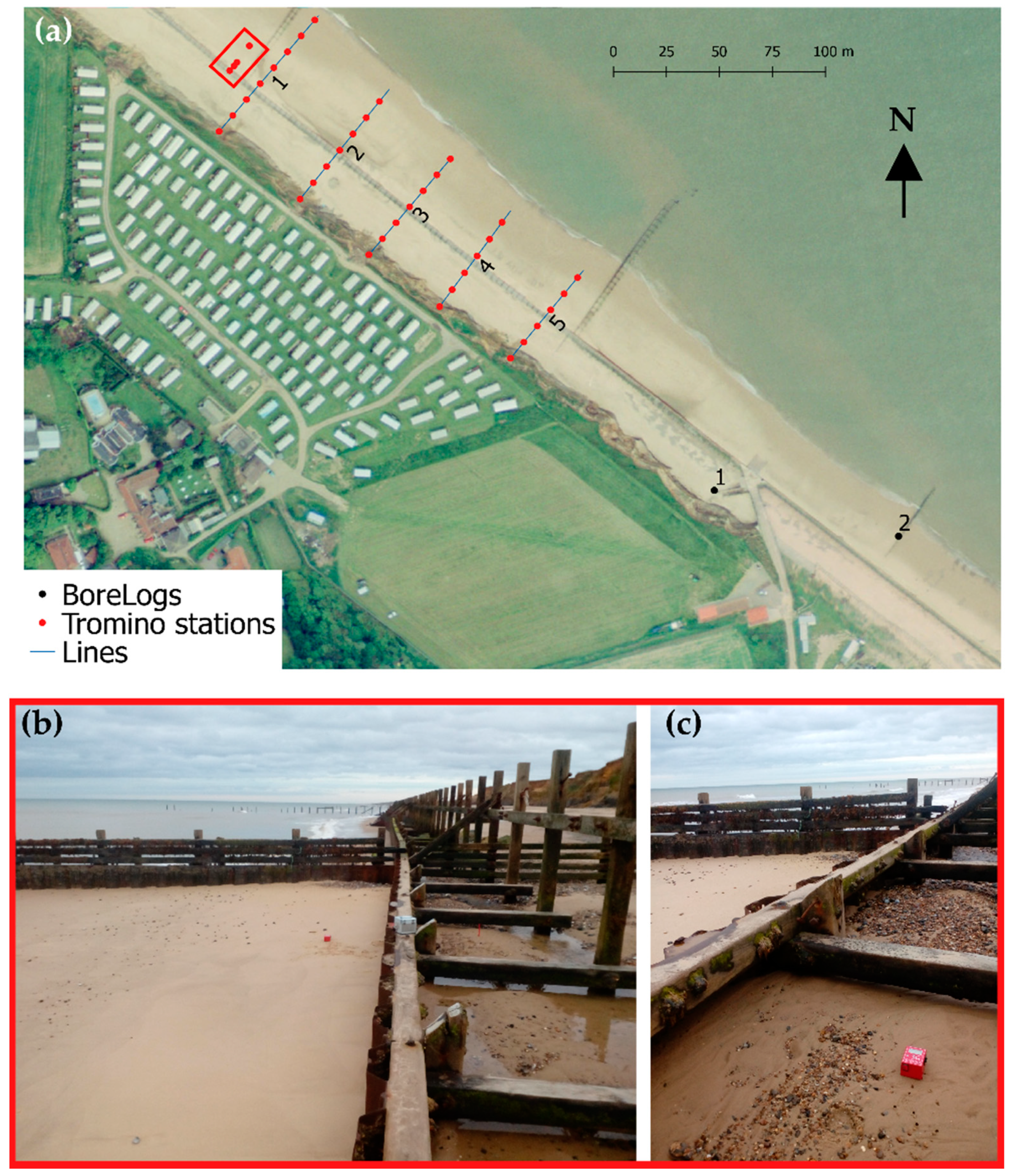
Passive seismic survey recorded locations; (a) 34 points along five lines (i.e., lines 1 to 5) were initially recorded covering the beach from the cliff toe to the seaward limit of the dry beach. Four additional points were recorded during the day, these are shown as points within a red rectangle; (b) detail of the extra station recorded immediately in front of the palisade and; (c) detail of extra station recorded immediately behind the palisade. Beach levels on stations shown in (a,c) were similar within ±10 cm.
Figure 6.
Passive seismic survey recorded locations; (a) 34 points along five lines (i.e., lines 1 to 5) were initially recorded covering the beach from the cliff toe to the seaward limit of the dry beach. Four additional points were recorded during the day, these are shown as points within a red rectangle; (b) detail of the extra station recorded immediately in front of the palisade and; (c) detail of extra station recorded immediately behind the palisade. Beach levels on stations shown in (a,c) were similar within ±10 cm.
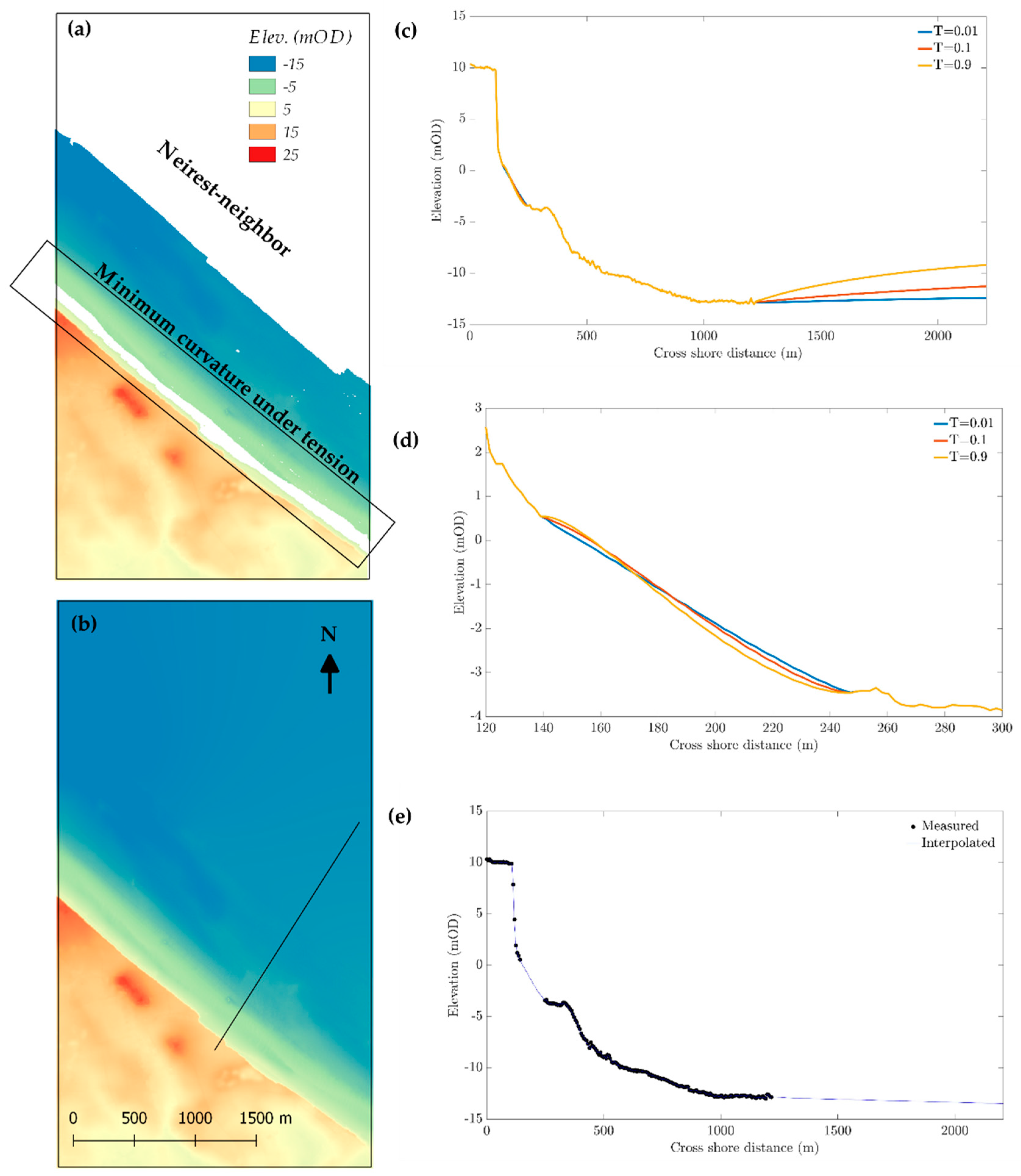
Figure 7.
DTM of study site: (a) EA-LIDAR inland topography year 1999 and EA-multibeam bathymetry year 2011 (white areas indicate data gaps); (b) interpolated DTM used in this work; (c) comparison of elevations along the transect shown by a solid black line in (b) using different tension parameter values (i.e., notice the unrealistic depth decrease seawards of ca. 1250 m cross-shore location); (d) detail of the upper shore-face interpolated bathymetries for different tension parameter values; (e) the final interpolated elevation along the same transect.
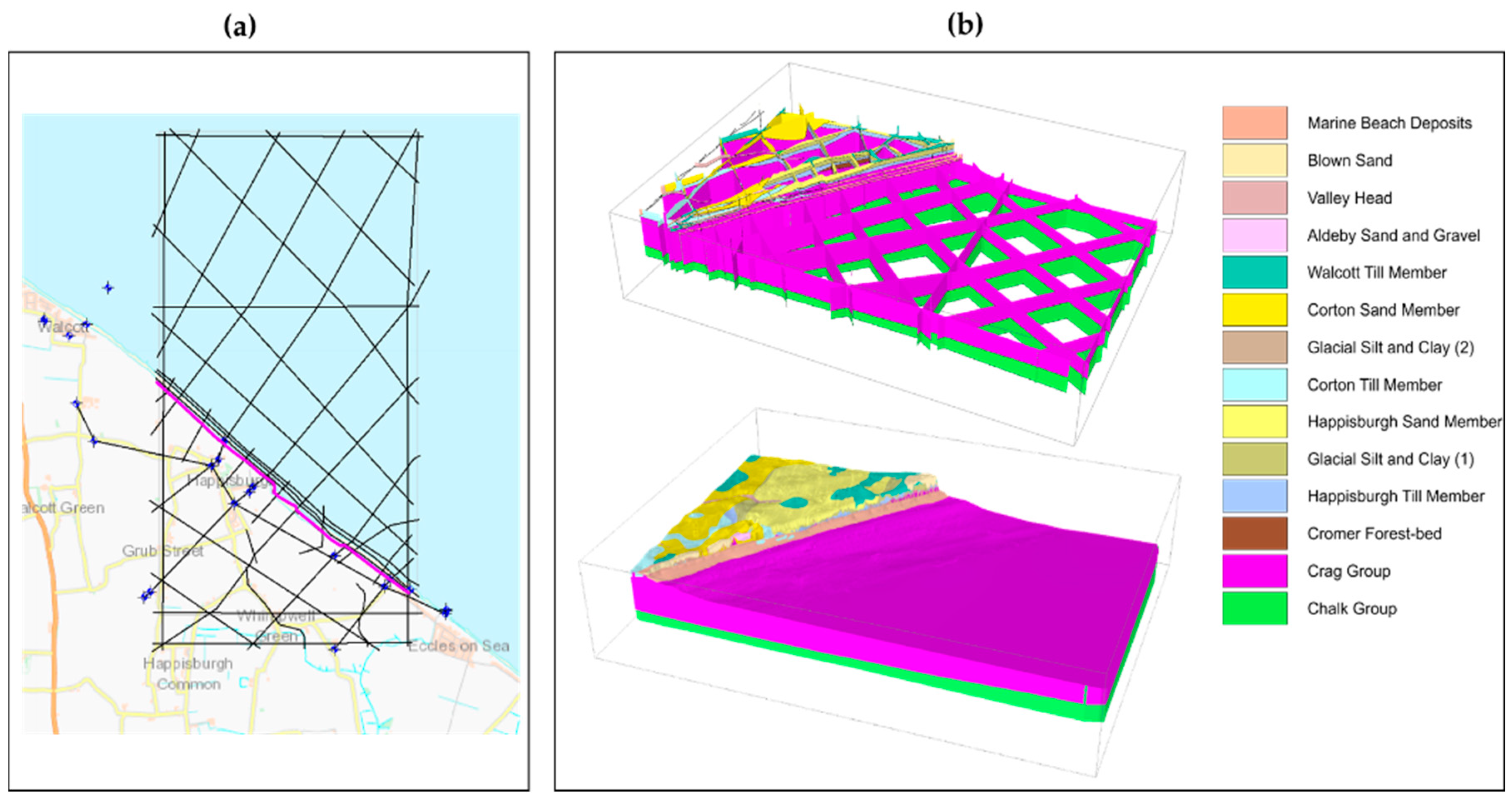
Figure 8.
Happisburgh 3D lithological model; (a) distribution of boreholes (blue circles) and cross-sections (black lines) used to construct the model, master coastal cross-section is highlighted in magenta; (b) upper panel shows all the cross sections with its interpreted geology and bottom panel shows the interpolated 3D lithological model.
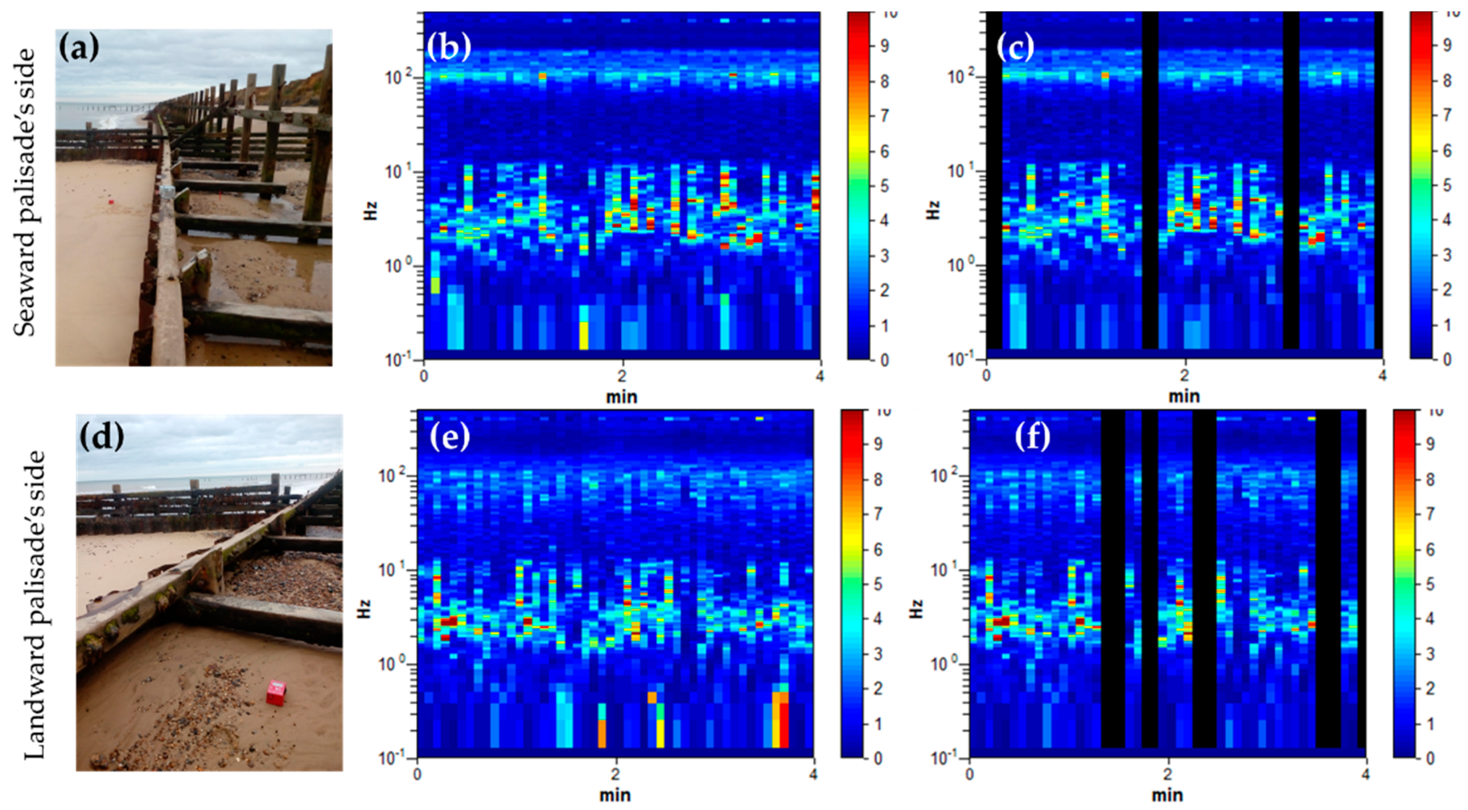
Figure 9.
Noise time history recorded and used to calculate the H/V spectra at both sides of the palisade: (a) location of the Tromino at the seaward side of the defence; (b) full record measured at the seaward side; (c) non-used noise data at the seaward side masked with black; (d) location of the Tromino at the landward side of the defence; (e) full record measured at the landward side; (f) non-used noise data at the landward side masked with black;.
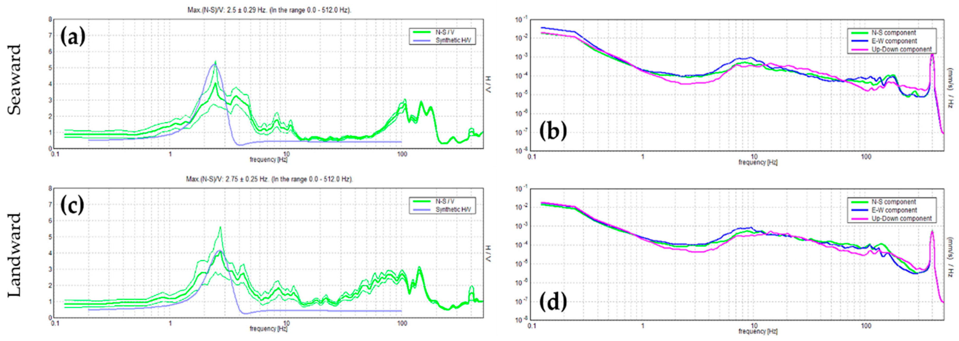
Figure 10.
N-S/V spectral ratio, synthetic N-S/V and single component spectra at the seaward and landward side of the palisade; (a) measured (green lines, where thick line is the average and thin lines are the standard deviation) and synthetic (blue line) N-S/V spectral ratio at the seaward side; (b) directional components spectra at the seaward side; (c) measured (green) and synthetic (blue) N-S/V spectral ratio at the landward side; (d) directional components spectra at the landward side.
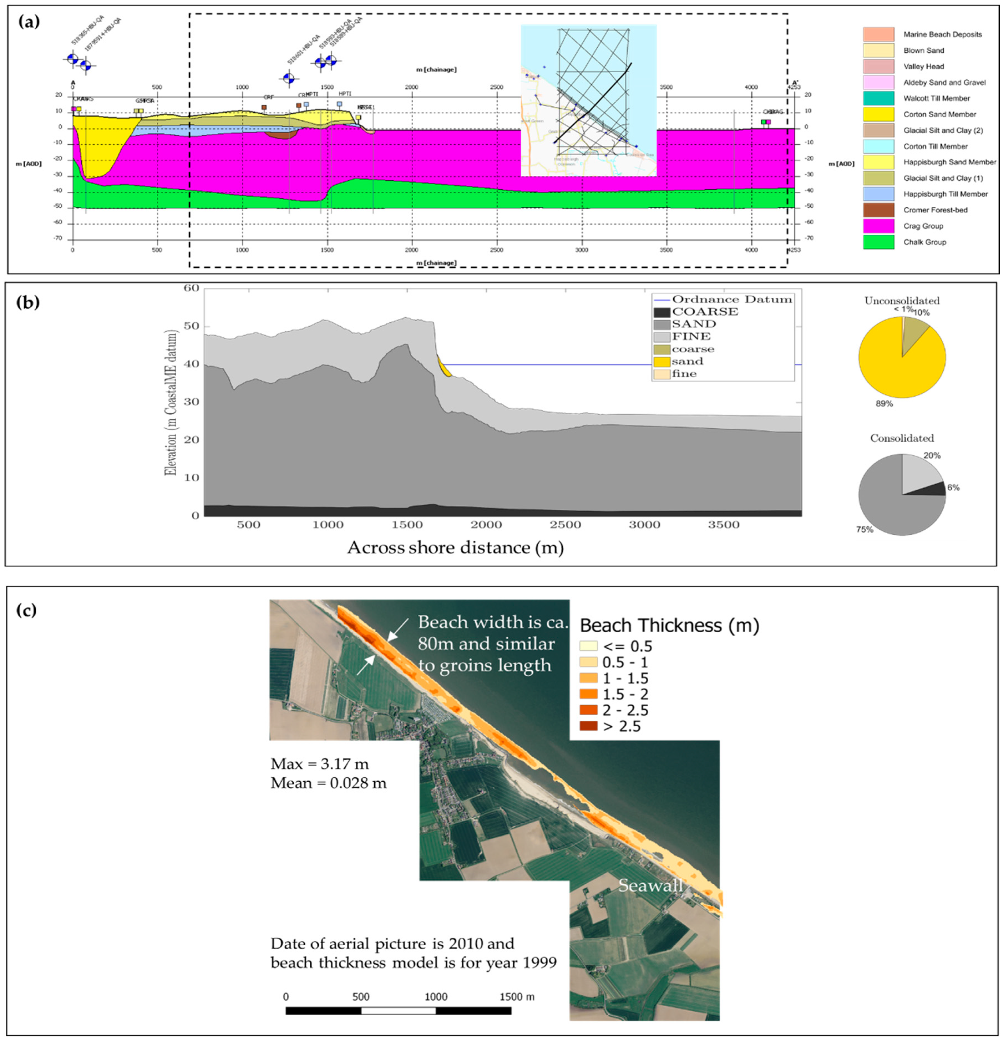
Figure 11.
Beach thickness at Happisburgh; (a) lithological model along a cross-section (section location shown as a thicker black line on small region map) showing the cliff and shore platform lithology; (b) combined profile elevation and percentage of different sediment sizes on consolidate and non-consolidated layers across a sub-domain of the lithological cross-section (sub-domain extension is indicated in panel (a) with a dashed rectangle). Total percentages of different sediment fractions shown as pie charts; (c) beach thickness along the Happisburgh coast.
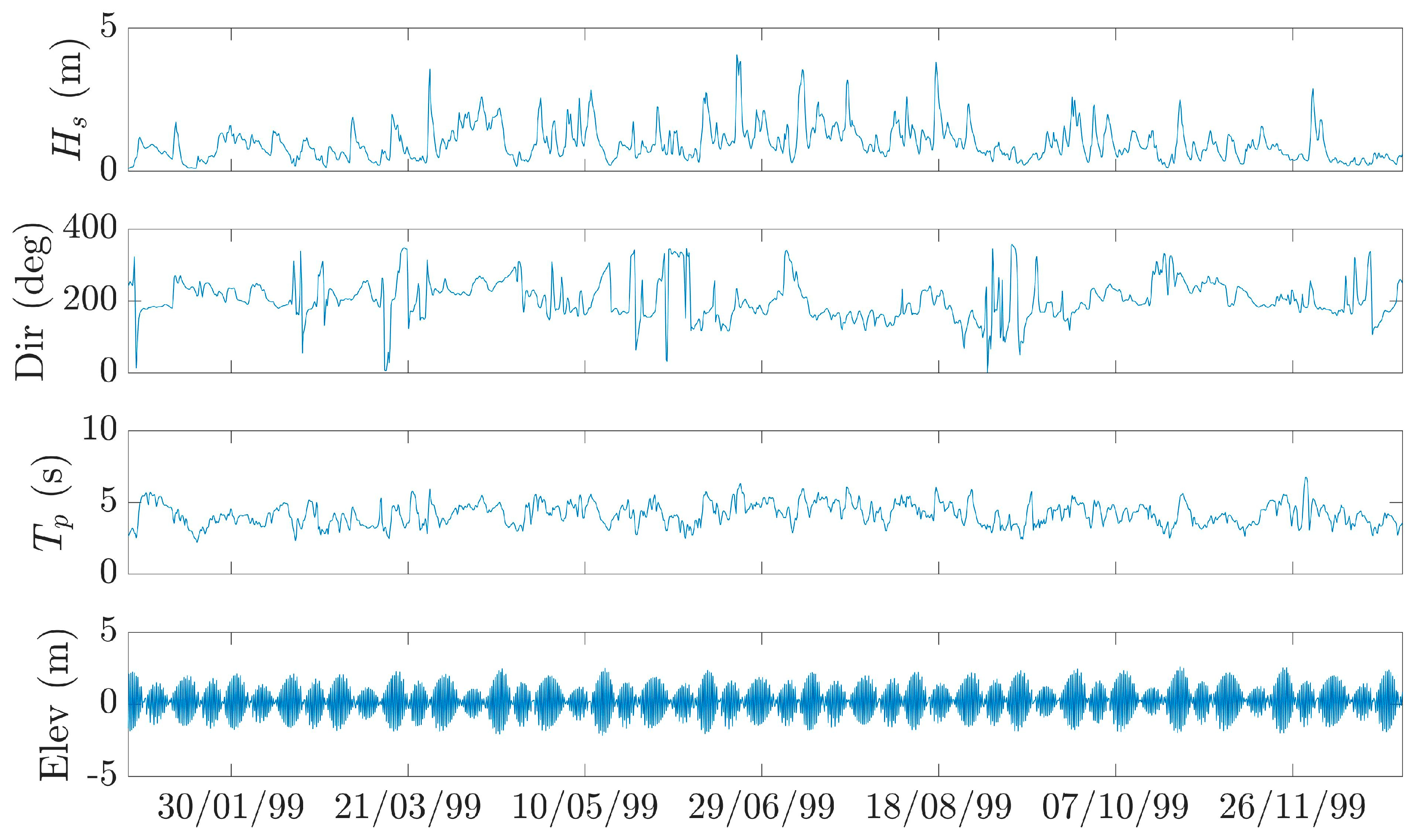
Figure 12.
Offshore wave and tidal elevation time series used as boundary conditions. The wave data is from the UKCP09 downscaled data at a point located 2.5 km offshore and 20 m depth of the study site. The elevation data are from the Cromer tide gauge station and referred to m above Newlyn datum.
Figure 12.
Offshore wave and tidal elevation time series used as boundary conditions. The wave data is from the UKCP09 downscaled data at a point located 2.5 km offshore and 20 m depth of the study site. The elevation data are from the Cromer tide gauge station and referred to m above Newlyn datum.
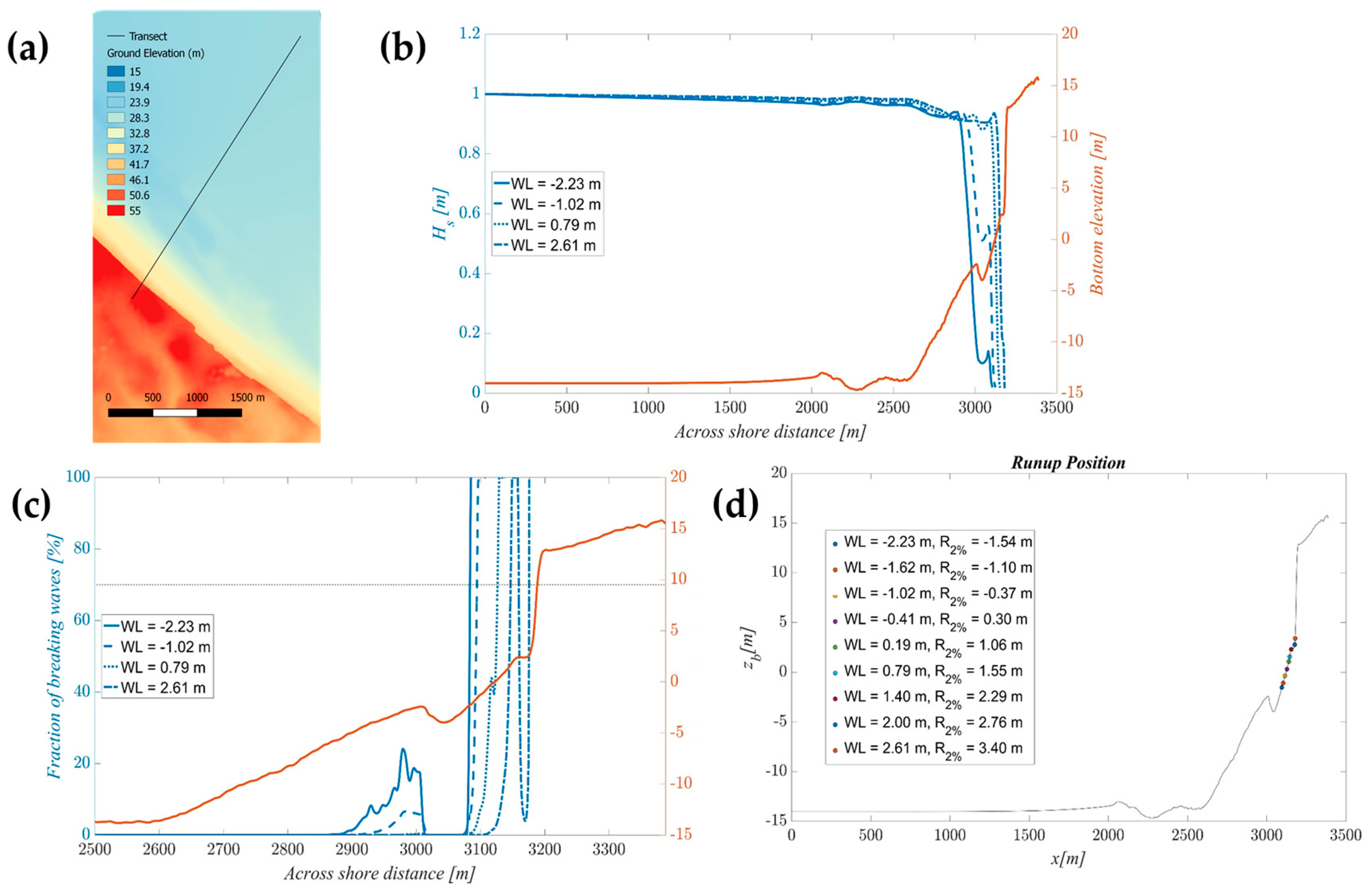
Figure 13.
CSHORE simulated wave propagation and run up along a representative Happisburgh transect; (a) location of the representative ca. 3.5 km long transect on the DEM of the study site; (b) significant wave height across-shore for different water levels along the representative transect; (c) percentage of waves breaking along the transect (the threshold of 70% used to estimate the surf zone width is represented as a dashed black line); (d) bottom profile elevation and wave run up values for each water level. The coloured circles represent the run up elevation intersection with the bottom profile.
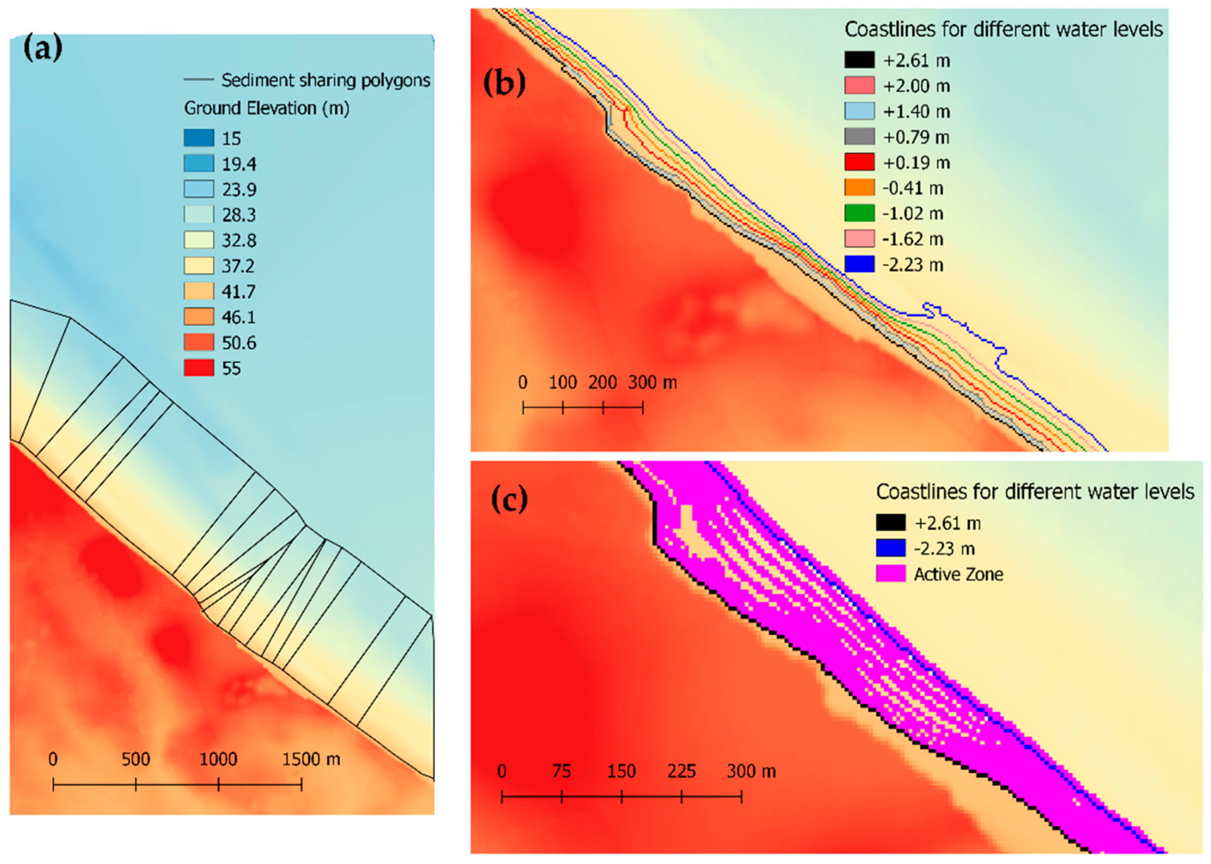
Figure 14.
Details of key modelling features over the full tidal range for the simulated year 1999; (a) shows the sediment sharing polygons that are automatically delineated at every time step. This figure shows the polygons for the shoreline delineated at the maximum water level (WL = +2.61 m); (b) delineated shoreline location at different water levels; (c) cells marked as active zones for all water levels shown in panel b. The shorelines for maximum and minimum water level are indicated for reference.
Figure 15.
Simulated beach volume accumulated changes. From top to bottom; eroded, deposited and net total sediment volume.
Figure 15.
Simulated beach volume accumulated changes. From top to bottom; eroded, deposited and net total sediment volume.
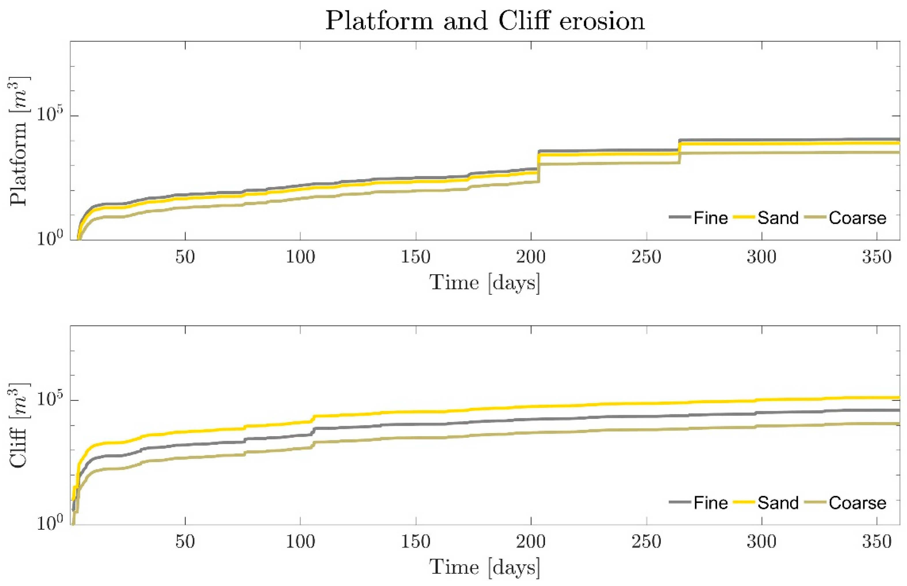
Figure 16.
Daily accumulated platform and cliff erosion sediment volume. All fine material eroded from the platform, cliff and beach becomes suspended sediment.
Figure 16.
Daily accumulated platform and cliff erosion sediment volume. All fine material eroded from the platform, cliff and beach becomes suspended sediment.
Figure 17.
Initial and final simulated beach thickness; (a) initial beach thickness derived from the lithological model; (b,c) details of the palisade in the northern side of the embayment and seawall on the southern side of the embayment respectively; (d–f) shows final beach thickness for different R values (indicated as [RPlatform, RCliff] (m9/4s2/3)); (g–i) shows the thickness difference between the final and initial beach thickness.
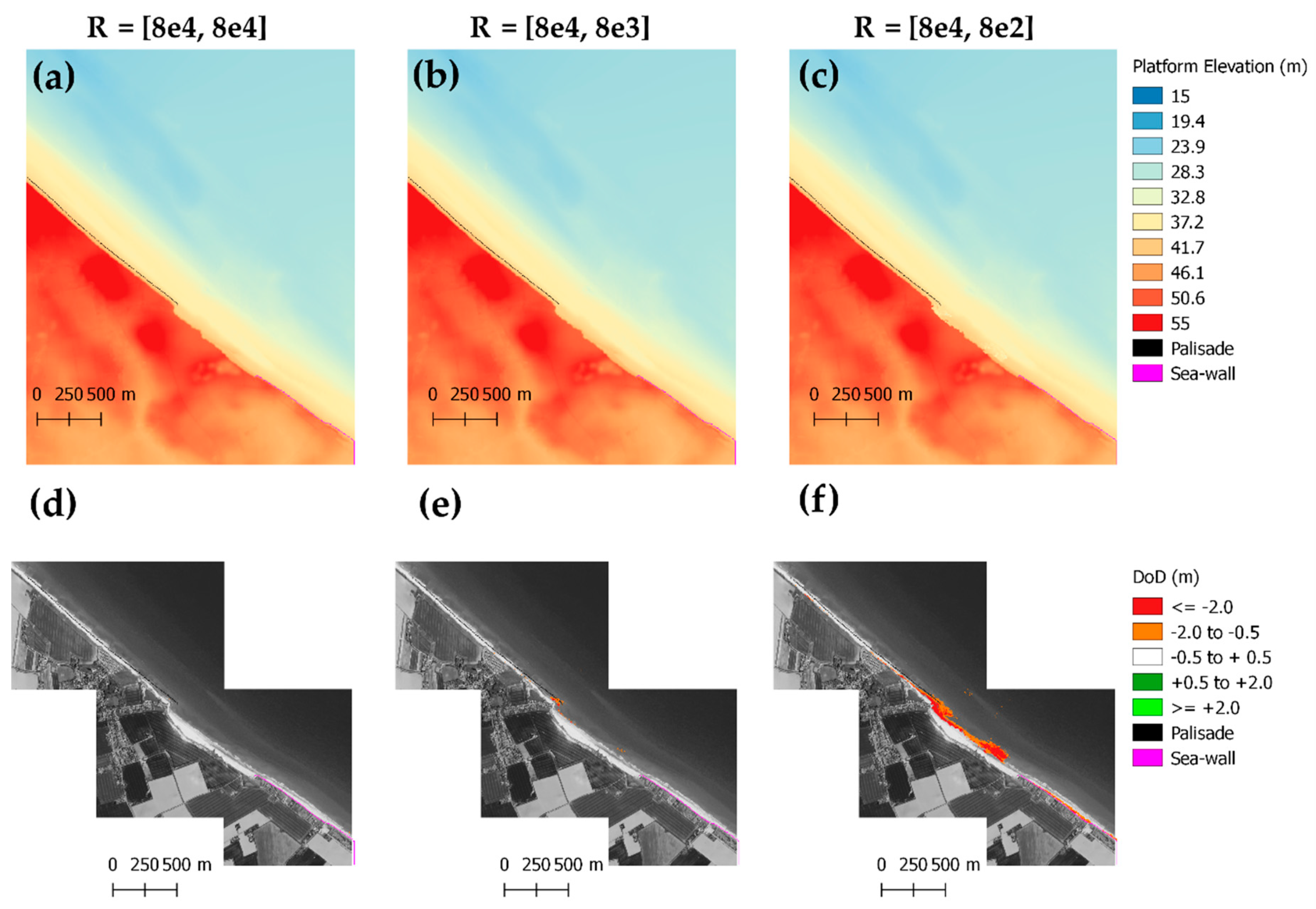
Figure 18.
Simulated final and net platform-elevation change; (a–c) final simulated platform elevation for different R-values (indicated as [RPlatform, RCliff] (m9/4s2/3)); (d–f) shows the digital elevation differences of platform elevation between the final and initial values.
Figure 18.
Simulated final and net platform-elevation change; (a–c) final simulated platform elevation for different R-values (indicated as [RPlatform, RCliff] (m9/4s2/3)); (d–f) shows the digital elevation differences of platform elevation between the final and initial values.
Table 1.
Component model, description and what element is implemented in CoastalME.
Table 1.
Component model, description and what element is implemented in CoastalME.
| Model | Method | Implementation in CoastalME |
|---|
| COVE | ‘one-line’ model designed to handle complex coastline geometries, with high platform curvature shorelines [29] | CoastalME as COVE, uses a local coordinate scheme (rather than global), and divide the coastline as a set of sediment sharing polygonal shapes (e.g., triangles and trapezoids). For each polygon, the potential alongshore sediment is calculated using CERC equation using polygon averaged breaking wave and sediment size properties. Actual alongshore sediment transport is constrained by unconsolidated sediment availability. |
| CSHORE | One-dimensional time-averaged near-shore profile model for predictions of wave height, water level, wave-induced steady currents, and beach profile evolution and stone structural damage progression [30]. | CoastalME propagates the wave properties by calling CSHORE hydrodynamic module along a number of cross-shore profiles. Wave properties between profiles are interpolated to provide polygon averaged values. |
| SCAPE | One line model which includes the beach and platform interactions. Its principal modules describe wave transformation, platform erosion, and a (one-line) beach [31,32]. | CostalME simulates beach and platform erosion as in SCAPE. The original horizontal SCAPE erosion is converted into its vertical component by applying a simple trigonometrical conversion (Equation (6) in [28]). |
Table 2.
CoastalME composition model inputs.
Table 2.
CoastalME composition model inputs.
| Input | Value |
|---|
| Required for a generic landscape evolution model | |
| Run duration | 360 days |
| Time step | 6 h |
| Wave heights, direction, period | UKCP09 hindcast data |
| Topo and bathymetric Digital Elevation Model | LiDAR year 1999 & Multibeam 2011 |
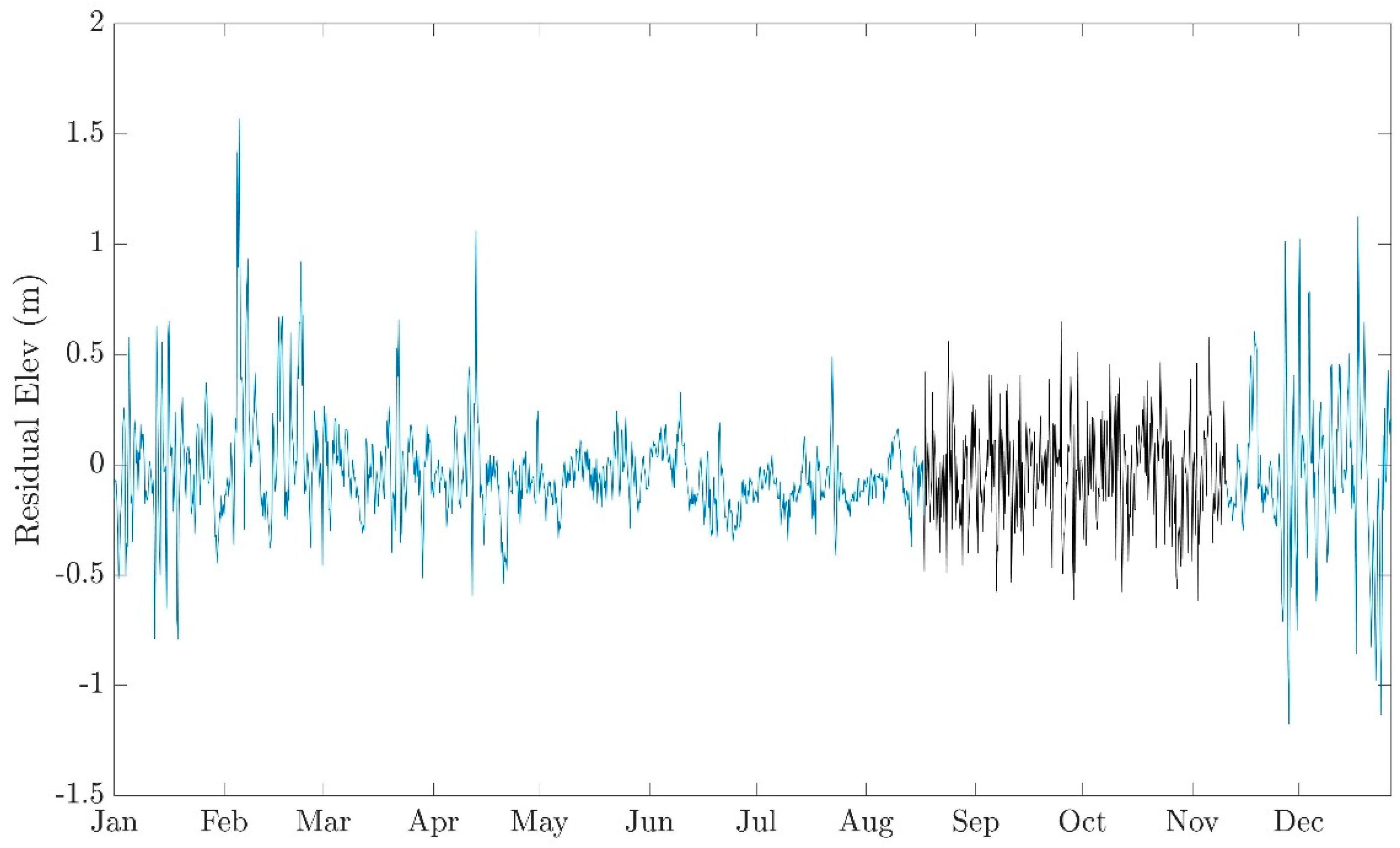
| Tides | Reconstruction of tidal signal using Cromer tide gauge data from 1999 to 2017 |
| Residual elevation | Difference of Cromer tide gauge elevation and tidal levels (gap filled assuming residuals follow a normal distribution) |
| CoastalME Datum | +40 m above basement level |
| Coarse, sand and fine sediment content | BGS thickness model |
| Coarse, sand and fine availability factor | 0.3; 0.7; 1.0 |
| Boundary conditions | Open boundaries (i.e., sediment at the boundaries is allotted to exit the grid but no external sediment inputs are assumed over the simulated period) |
| Required for COVE-sediment sharing module | |
| CERC coefficient | 0.79 |
| Length of normal profiles used to create the polygons | 800 m |
| Required for CSHORE-wave propagation module | |
| Breaker ratio parameter γ | 0.8 |
| Friction factor fb | 0.015 |
| Required for SCAPE-beach & platform interaction | |
| Rock strength and hydrodynamic constant, R | RPlatform = 8 × 10⁴ [m9/4s2/3]
RCliff = 8 × 10² [m9/4s2/3] |
| Beach volume & and beach thickness | Derived from BGS thickness model |
| Full list of parameters provided in Table S1 |
Table 3.
Total accumulated annual platform erosion, cliff collapse, beach erosion, beach deposition and suspended sediment.
Table 3.
Total accumulated annual platform erosion, cliff collapse, beach erosion, beach deposition and suspended sediment.
| Platform Erosion |
| Total potential platform erosion = 25,612.27 m3 |
| Total actual platform erosion = 22,584.25 m3 |
| Total fine actual platform erosion = 11,292.12 m3 |
| Total sand actual platform erosion = 7904.49 m3 |
| Total coarse actual platform erosion = 3387.64 m3 |
| Cliff Collapse |
| Total cliff collapse = 181,708.20 m3 |
| Total fine cliff collapse = 40,646.87 m3 |
| Total sand cliff collapse = 129,436.91 m3 |
| Total coarse cliff collapse = 11,624.42 m3 |
| Beach Erosion |
| Total potential beach erosion = 88,958.33 m3 |
| Total actual beach erosion = 6244.53 m3 |
| Total actual fine beach erosion = 133.40 m3 |
| Total actual sand beach erosion = 4774.00 m3 |
| Total actual coarse beach erosion = 1337.13 m3 |
| Beach Deposition |
| Total beach deposition = 17,376.80 m3 |
| Total sand beach deposition = 12,660.11 m3 |
| Total coarse beach deposition = 4716.69 m3 |
| Suspended Sediment |
| Suspended fine sediment = 1415.153 m3 |
| Simulation results for model setup as shown in Table 2 |
Table 4.
Initial and simulated changes of sediment volumes; total, beach and platform.
Table 4.
Initial and simulated changes of sediment volumes; total, beach and platform.
| | Initial (m3) | Change (m3) |
|---|
| Total | 392.559,461 | −252,343 |
| Beach (un consolidated) | 342,622 | −112,419 |
| Platform (consolidated) | 392,256.014 | −179,099 |
| Suspended sediment | 0 | +52,072 |
| Simulation results for model setup shown in Table 2 |

 ,
, 


