1. Introduction
The impact of mineral oil pollution is a widely spread source of environmental concern in various ecosystems [
1,
2]. The detection of the sea surface expression of oil using space-borne surveillance systems is an extensively studied subject [
3,
4,
5]. Oil floating on the surface of the ocean can be located, to some extent, with different types of remote sensing sensors—e.g., thermal infrared (AVHRR: Advanced Very High Resolution Radiometer [
6]), visible/near infrared (MODIS: Moderate Resolution Imaging Spectroradiometer [
7]), etc.—but generally, most attempts concentrate on using satellite-derived measurements from active microwave-imaging instruments (SAR: Synthetic Aperture Radars [
8,
9,
10]), e.g., RADARSAT [
11,
12].
Research projects using SAR measurements to study petrogenic oil slicks usually focus on understanding two major processes: (1) Identification of smoother regions observed at the sea surface with reduced radar backscattering signal, i.e., classification and segmentation for dark spot detection (e.g., [
13]); and (2) Differentiation of radar signature of mineral oil slicks from what is commonly referred to as “radar look-alikes” (e.g., [
14])—for instance, surface natural oil produced by plants or animals (i.e., biogenic oil films), atmospheric conditions (e.g., low wind and rain cells), oceanographic features (e.g., upwelling regions and internal gravitational waves), etc. [
15]. Apart from the scientific effort studying these two processes [
16], few investigations are directed at using remote sensing systems to differentiate the mineral oil-slick type—i.e., differences among types of anthropogenic oil slicks observed at the sea surface, for instance: oil slicks formed from heavy versus light oil [
17]; or oil slicks from production oil tests (i.e., oil released at the surface of the ocean in the process of evaluating new drilling wells) versus oily water (i.e., oil slicks from leakages occurring during the exploration or production phases) [
18].
The available literature covering the subject of identifying oil slicks at the surface of the ocean using space-borne surveillance systems, for the most part, does not address the petrogenic oil-slick category discrimination: telling apart the oil-slick sea surface expression in relation to their source, thus considering oil seeps (i.e., natural oil seepages from a hydrocarbon reservoirs) versus oil spills (i.e., mineral oil spillages from man-made activities) [
19,
20,
21,
22]. The seep-spill discrimination mostly regards two points of view: economic and environmental. While the former deals with the discovery of new oil exploration frontiers in finding the presence of active petroleum systems, the latter is capable of improving the relationship between the oil- and gas-related industry and environmental organizations (and society as a whole) by reducing any origin uncertainty about the oil slick source (i.e., naturally-occurring seeps versus man-made spills). A third point of view is the one of the remote sensing community, in which if a certain methodology is capable of discriminating oil from oil using microwave measurements acquired from space [
19,
20,
21,
22], it might be plausible to say that such methodology can also be applied to differentiate oil from look-alike features in SAR imagery. This framework scientifically strengthens the other two points of view.
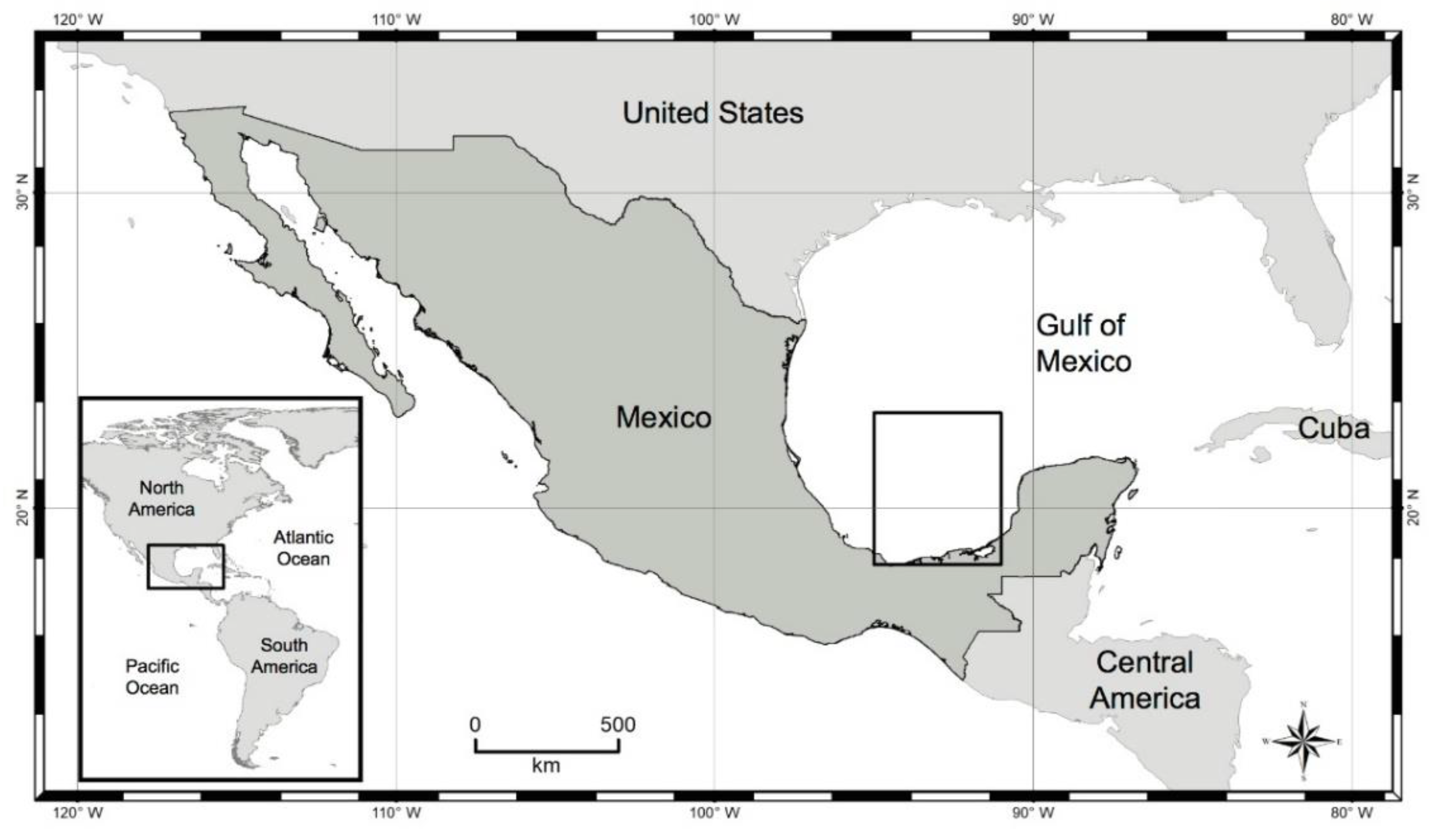
Notwithstanding the relative neglect of research projects on the use of satellite sensors for the discrimination of the oil-slick category, Carvalho [
19] showed it is feasible to use SAR-derived measurements for seep-spill discrimination—see also [
20,
21,
22]. These authors have used a series of Multivariate Data Analysis Techniques to devise a novel idea to discriminate the oil-slick category while studying seeps and spills observed on the surface of the ocean in the Gulf of Mexico off the Mexican coast in the Campeche Bay region (
Figure 1). They have proposed a simple Oil-Slick Discrimination Algorithm based on SAR backscatter signature, i.e., sigma-naught (σ
o), beta-naught (β
o), and gamma-naught (γ
o) [
23,
24,
25], along with the geometry, shape, and dimension of the oil slicks. Their best outcome is reached with optimal Overall Accuracies of approximately 70%, based on the oil slicks’ areas and perimeters.
We report on analyses to refine the ability to discriminate the petrogenic oil-slick category (seeps versus spills) proposed in our previous investigations [
19,
20,
21,
22]. Exploiting the same dataset, but with expanded Data Processing Segments, we extend our earlier studies onto a firmer basis. Based on our methodical data mining exercise, we seek to improve the seep-spill discrimination accuracy, as well as to answer three scientific questions:
Among the several Data Transformation Approaches we tested, which one provides the most accurate oil-slick category discrimination?
Is there a specific Attribute Selection Process that excels at choosing variables to discriminate seeps from spills?
Which combination of Oil-Slick Information Descriptors promotes the best discrimination between seeps and spills?
2. Methods
We developed a comprehensive Exploratory Data Analysis (EDA) to reveal hidden information contained in the satellite-derived measurements and to refine the analysis to discriminate slicks by category, as proposed in our earlier studies [
19,
20,
21,
22]. The design of our EDA focuses on a data-driven scheme to investigate possible ways to improve the seep-spill discrimination with the simplest possible analysis and the lowest satellite-imaging cost. The research strategy employed herein is a development of our previous investigations [
19,
20,
21,
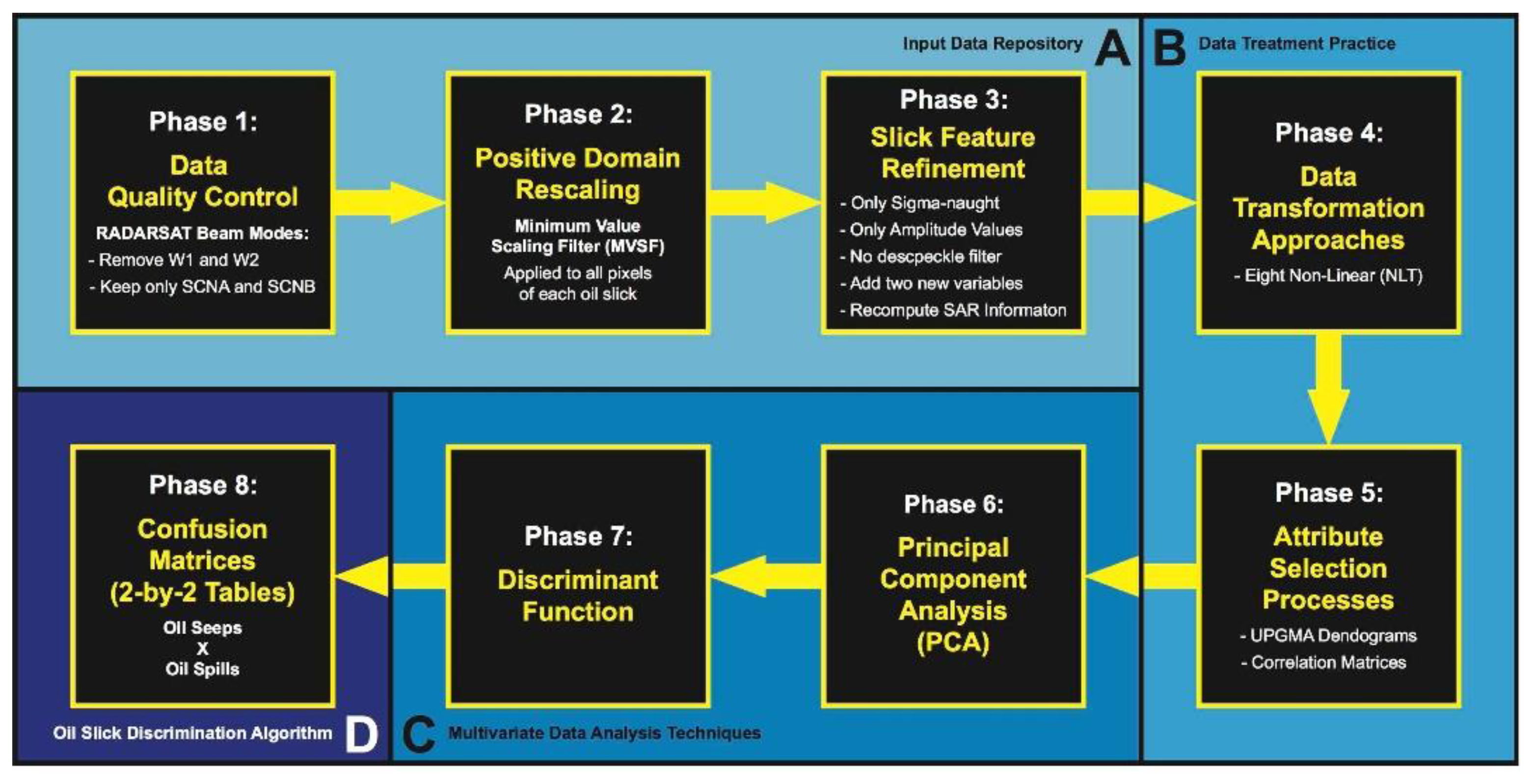
22], and consists of four distinct Data Processing Segments (i.e., A, B, C, and D in
Figure 2)—devised in eight individual Phases—separately described in detail and introduced in a complete manner easily enabling replicability of our data mining exercise. A summary of our EDA design is depicted in
Figure 2. While in-house Python codes are used to run the oil slick RADARSAT-2 related analyses (i.e., Phases 1–4), PAST (PAleontological STatistics: version 3.20, Oslo, Norway [
26]) is used in the implementation of Phases 5–8.
A multi-year dataset of RADARSAT-2 scenes imaged between 2008 and 2012 gave rise to the oil slick data archive analyzed in our earlier investigations [
19,
20,
21,
22]. This data archive consists of polygons representative of oil slicks that had been identified and field validated as seeps and spills by domain experts. For more information about this dataset, see [
19,
20,
21,
22]. The workable dataset explored herein is defined after fine-tuning this data archive along the 1st Data Processing Segment (
Figure 2A: Input Data Repository—Phases 1–3).
2.1. Phase 1: Data Quality Control
The initial oil slick data archive from our previous studies [
19,
20,
21,
22] is sorted by the satellite scene-imaging configuration (i.e., beam modes determining the acquisition swath width and ground resolution), thus establishing the amount of RADARSAT-2 imagery and the seeps and spills of our workable dataset.
2.2. Phase 2: Positive Domain Rescaling
The initially available oil slick data archive analyzed in our earlier investigations [
19,
20,
21,
22] had undergone a linear scaling action (Negative Values Scaling Filter: NVSF) that is comprised of a two-fold procedure applied to individual oil slicks: the subtraction of the minimum negative pixel value within each oil slick from every single pixel of such oil slick, followed by the addition of 1 to every single pixel—the minimum pixel value becomes 1. This brings all pixel values to the positive domain, which is a requirement of data normalization procedures that cannot be applied to negative values, e.g., log
10. The NSVF is applied at the pixel level, i.e., taking into account all pixels of each oil slick to provide a single measure representative of all pixels of such oil slick (see below:
Section 2.3.2). Nevertheless, previously, the NVSF was only applied to certain oil slicks: those having at least one negative pixel value—for instance, oil slicks that had spurious negative SAR backscatter signature caused by intrinsic multiplicative random granular speckle noise destructive imprecision in the range-dependent gain calculation [
27,
28].
Although we also conduct this filtering strategy, we apply it in the present research to all oil slicks. In essence, hereafter, for our purpose, the NVSF is referred to as Minimum Values Scaling Filter (MVSF), such that: PIXpos = (PIX-PIXmin) + 1, in which PIXpos corresponds to the new positive pixel value, PIX is the original pixel value, PIXmin is the minimum pixel value of all pixels of each oil slick. Therefore, this is a dissimilarity between our previous investigations and the current EDA: NVSF versus MVSF. The reason for applying the MVSF to all oil slicks is three-fold: (1) To avoid possible biases caused by gradient differences among oil slicks with and without NVSF; (2) To circumvent the application of despeckle filtering (e.g., Frost Filter: FFrost [
29]; see also Phase 3) that eventually would eliminate negative values, but would alter (e.g., smoothing) the SAR backscatter signature values—the lack of such filter is justifiable to preserve the data-driven design of our EDA; and (3) To exploit data transformations that do not accept negative values (see below: Phase 4).
2.3. Phase 3: Slick Feature Refinement
2.3.1. SAR Backscatter Signature
Previously, we explored twelve SAR backscatter signatures: SAR backscatter coefficients corresponding to the radar cross-section (RCS: σ) normalized by the unit area calculated in three different surface planes (i.e., σ
o, β
o, and γ
o [
30,
31,
32,
33,
34]) computed in four radiometric-calibrated image products—i.e., the amplitude (1st) of the received radar beam and its dimensionless physical quantity form that represents power expressed in dB (2nd), both with (3rd) and without (4th) despeckle filtering (FFrost: 3-by-3 window). However, herein we perform a simplification for a more controlled EDA solely using σ
o given in amplitude without despeckle filtering. As such, from this point onwards, unless otherwise stated, any reference to SAR backscatter signature synonymously refers to this simplification.
2.3.2. Oil-Slick Information Descriptors
As before [
19,
20,
21,
22], we start our research analyzing the same ten attributes describing the oil slicks’ geometry, shape, and dimension (these are collectively referred to as Size Information Descriptors) derived from two basic morphological features characterizing the oil slicks—i.e., area (Area) and perimeter (Per):
Analogously, we also exploit the same 36 basic descriptive statistics metrics experimentally explored to characterize the oil slicks’ SAR backscatter signature as in our previous investigations [
19,
20,
21,
22]. These metrics are calculated based on all pixels inside individual oil slick polygons:
Four central tendency measures: Average (AVG), Median (MED), Mode (MOD), and Mid-mean (MDM: mean of the values between the 2nd and 3rd interquartiles, i.e., it trims off 25% of both ends);
Six measures of dispersion: Range (RNG), Coefficient of Dispersion (COD: the subtraction of the 1st interquartile from the 3rd interquartile and the division by their sum), Standard Deviation (STD), Variance (VAR), Average Absolute Deviation (AAD: mean of the absolute difference of each value to the mean), and Median Absolute Deviation (MAD: median of the absolute difference of each value minus the median);
24 pair-values of Coefficients of Variation (COV: ratio between STD and AVG [
18], such that each of the six dispersion measures are individually divided by the four central tendencies);
The Minimum (MIN) and Maximum (MAX) pixel values of each oil slick.
Herein we introduce two new variables that describe the distribution patterns of the pixels within each oil slick: Skewness (SKW) and Kurtosis (KUR). As such, this collection of 38 basic descriptive statistics metrics characterizing the oil slick’s SAR backscatter signature is henceforth referred to as SAR Information Descriptors. Together, these two types of Oil-Slick Information Descriptors (i.e., Size and SAR) determine the initial number of variables (48) accounted in our workable dataset.
2.4. Phase 4: Data Transformation Approaches
In contrast with our previous investigations [
19,
20,
21,
22], which implemented only a single non-linear normalization (log
10) and one linear standardization (Ranging [
40]), we exploit several Non-Linear Transformations (NLTs [
41,
42,
43,
44]):
NLT.0: No Transformation (x);
NLT.1: Reciprocal (1/x);
NLT.2: Logarithm Base 10 (log10(x));
NLT.3: Napierian Logarithm (Ln(x));
NLT.4: Square Root (x1/2);
NLT.5: Square Power (x2);
NLT.6: Cube Root (x1/3);
NLT.7: Third Power (x3).
In which x corresponds to the actual value of each oil slick variable (i.e., Oil-Slick Information Descriptors—see Phase 3). Half of these (i.e., NLT.1, NLT.2, NLT.3, and NLT.4) do not accept negative values (x). To simplify our analyses, we do not perform linear standardizations.
2.5. Phase 5: Attribute Selection Processes
The processes of selecting relevant attributes deals with the complex matter of reducing dimensionality in the variable-hyperspace domain (see also Phase 6); this generally helps to elucidate the problem solution of numerical ecology assessments and to improve the performance of classification algorithms [
42,
45]. As such, another difference from our earlier studies is the number of explored attributes: before, we investigated 44 data sub-divisions with 502, 433, 423, 151, 141, 35, 10, and 2 variables [
19,
20,
21,
22]. Indeed, we considerably reduce these numbers with the SAR backscatter signature simplification (see Phase 3:
Section 2.3.1). Additionally, we start with 48 Oil-Slick Information Descriptors (see Phase 3:
Section 2.3.2) but use even fewer variables upon the completion of the Attribute Selection Processes (see below:
Section 2.5.1).
2.5.1. Unweighted Pair Group Method with Arithmetic Mean (UPGMA)
Two attribute selection strategies (i.e., R-mode) have been performed in our previous investigations [
19,
20,
21,
22]: UPGMA [
42,
43,
46] and CFS (Correlation-Based Feature Selection [
47,
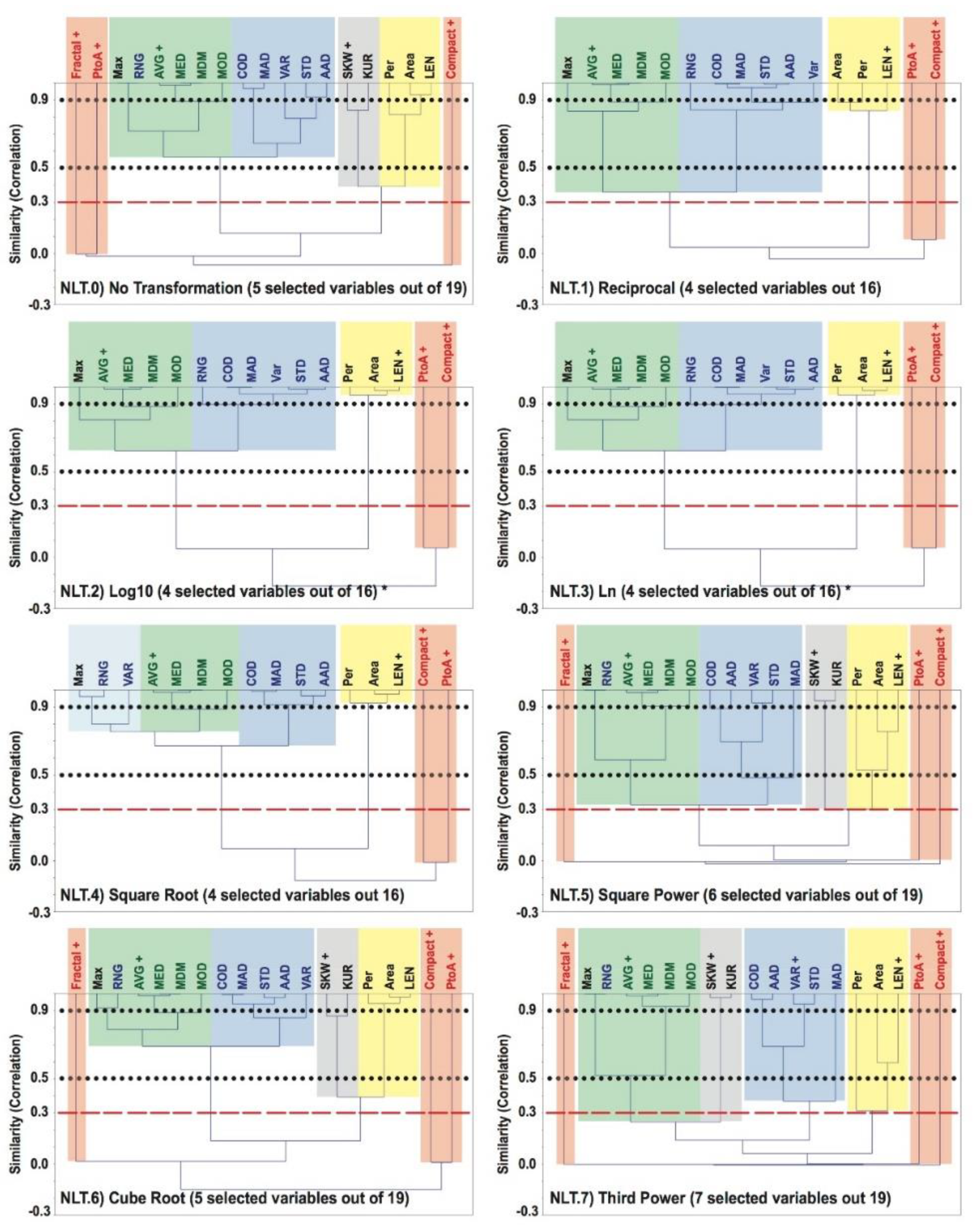
48]). Based on our earlier results, we only implement the former as it allows a user-defined strategy to select relevant variables: the choice of the similarity index (Pearson’s r correlation coefficient) used in the UPGMA dendrogram as cut-off to form groups of similar variables, i.e., phenon line [
49,
50]. See also [
19,
20,
21,
22] for further information about analyses and interpretations of rooted tree UPGMA dendrograms.
Moreover, an imperative distinction from our earlier investigations is that herein we are experimenting the use of a strict cut-off level, i.e., a fixed similarity value of 0.3, in relation to the previous fixed value of 0.5 and varying one ranging around 0.9 [
19,
20,
21,
22]. The selection of the 0.3 similarity cut-off is enlightened by the Bonferroni Adjustment as the level of minimum significance (
p value) for large datasets (
n > 100); below this there is no statistically significant correlation and variables are considered different from one another [
51].
2.5.2. Histograms and Correlation Matrices
Histograms and correlation matrices assist in the verification of residual inter-variable correlation and to help with the decision of which variables to select on the groups formed on the UPGMA analyses.
2.6. Phase 6: Principal Component Analysis (PCA)
PCAs reduce the large correlated variables set into a smaller set of uncorrelated hypothetical variables—Principal Components (PCs)—containing most of the relevant information of the initial larger set [
42,
43]. The rotation of the original axes to the new orthogonal coordinate system is implemented in the same manner as our earlier work: square symmetric correlation matrix and 1000 bootstraps [
52]. However, the approach to select relevant axes (i.e., PCs) is a departure from our earlier investigations. While, herein we use only the Kaiser Cut, i.e., Kaiser-Guttman criterion (eigenvalues > 1 [
53]), previously we explored several PC-selection practices, e.g., Jolliffe, Scree Plot (Knee/Elbow), and a combined strategy using the Scree Plot (broken stick) with Kaiser [
54,
55,
56,
57].
2.7. Phase 7: Discriminant Function
Discriminant Analysis differs from Clustering Analysis as it is not meant to determine to which group each object belongs [
43]. Instead, Discriminant Functions use a priori measured information (Oil-Slick Information Descriptors) and knowledge of the object’s (oil slick) group membership (seep or spill), to obtain the maximum discriminating power that minimizes the probability of erroneous discrimination: [DF(X) = (W
1X
1 + W
2X
2 + … + W
nX
n)−C
off]; in which DF(X) corresponds to the dependent variable (i.e., Discriminant Function); X
n to the independent variables (i.e., Oil-Slick Information Descriptor value); W
n to the independent variables’ weight; and C
off to the constant offset [
58,
59,
60,
61].
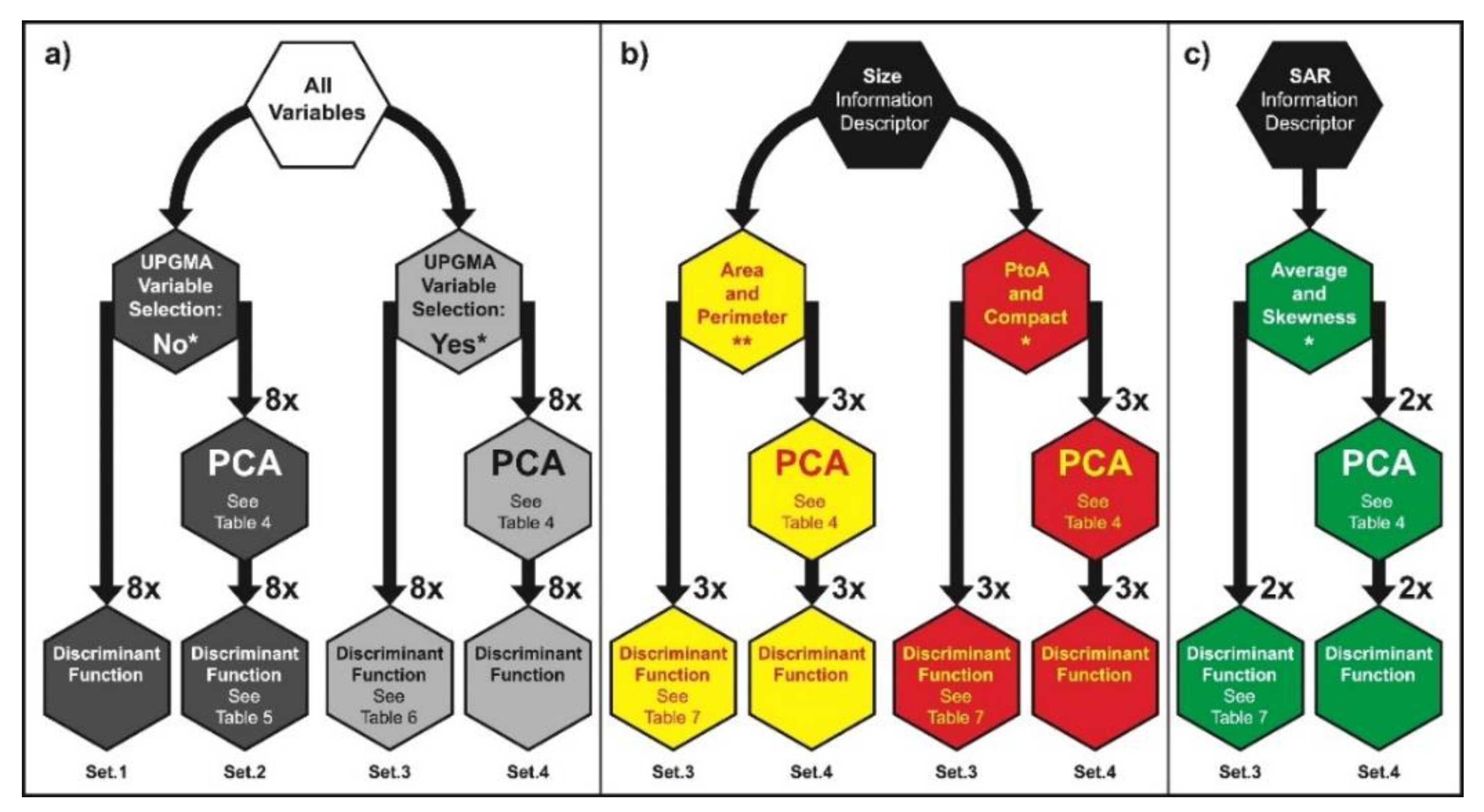
The use of uncorrelated attributes (selected PCs from Phase 6), or at least with the lowest possible degree of dependence (UPGMA selected variables from Phase 5), is a pressing need for Discriminant Functions [
62], and as such, this concerns a crucial development of the current EDA from our previous investigations [
19,
20,
21,
22]: herein, we are not only using the PCA scores (PCs) as input to the Discriminant Functions, we are also testing the use of UPGMA dendrogram selected variables (see Phase 5:
Section 2.5.1) without passing through the PCA.
2.8. Phase 8: Confusion Matrices (2-by-2 Tables)
The Oil-Slick Discrimination Algorithm accuracy is reported based on the Discriminant Function results by means of the complete understanding of adapted 2-by-2 Tables (Confusion Matrices: CMs). See also [
19,
20,
21,
22,
63,
64,
65] for information on how to analyze and to better interpret 2-by-2 Tables. The conjunct interpretation of five metrics [
66] is essential to fully evaluate the algorithm’s effectiveness.
Table 1 gives a picture of these metrics that are color-coded for clarity:
CM.1: Overall Accuracy (shown in Green);
CM.2: Producer’s Accuracy (i.e., Sensitivity and Specificity—shown in Yellow);
CM.2: Commission Error (i.e., False Negative and False Positive);
CM.3: User’s Accuracy (i.e., Positive and Negative Predictive Values—shown in Purple);
CM.3: Omission Error (i.e., Inverse of the Positive and Negative Predictive Values).
4. Conclusions
Our research addresses a gap in our scientific knowledge regarding the discrimination of the oil-slick category, i.e., sea surface expression of oil seeps versus oil spills observed in Campeche Bay (
Figure 1). We report on analyses to refine the ability of using SAR-derived measurements for this task, thus addressing expanded Data Processing Segments (A, B, C, and D in
Figure 2) as compared to our previous investigations [
19,
20,
21,
22]. A firmer basis to discriminate slicks by category has been established with the specific data-driven design of our Exploratory Data Analysis (EDA). An innovative strategy to select uncorrelated attributes based on the Bonferroni Adjustment (i.e., Pearson’s r correlation coefficient of 0.3 [
51]) has been successfully implemented using rooted tree dendrograms (Unweighted Pair Group Method with Arithmetic Mean: UPGMA—see
Figure 3). We investigate several Non-Linear Transformations (NLTs—see Phase 4: Data Transformation Approaches) and various strategies to select uncorrelated attributes: we tested more than 32 combinations of Data Transformation Approaches, i.e., eight NLTs versus four input dataset versions (see Set.1, Set.2, Set.3, and Set.4 in Phase 7: Discriminant Function—
Figure 4).
Based on our comprehensive approach to find a simple way to discriminate seeps from spills, we are able to answer the three scientific questions:
Our EDA also demonstrates that using simple and low-cost RADARSAT-2 beam modes (SCNA and SCNB), one can achieve useful seep-spill discrimination accuracies, thus supporting new products for the RADARSAT Constellation Mission (RCM): RADARSAT-2 Mode Selection for Maritime Surveillance (R2MS2).

 ,
, 


