Abstract
A three-dimensional numerical study of the hydrodynamic effect produced by a system of submerged breakwaters in a coastal area with a curvilinear shoreline is proposed. The three-dimensional model is based on an integral contravariant formulation of the Navier-Stokes equations in a time-dependent curvilinear coordinate system. The integral form of the contravariant Navier-Stokes equations is numerically integrated by a finite-volume shock-capturing scheme which uses Monotonic Upwind Scheme for Conservation Laws Total Variation Diminishing (MUSCL-TVD) reconstructions and an Harten Lax van Leer Riemann solver (HLL Riemann solver). The numerical model is used to verify whether the presence of a submerged coastal defence structure, in the coastal area with a curvilinear shoreline, is able to modify the wave induced circulation pattern and the hydrodynamic conditions from erosive to accretive.
1. Introduction
Submerged breakwaters are usually designed to defend the coastline from the erosion induced by breaking waves. The introduction of a system of submerged breakwaters separated by gaps produces two hydrodynamic effects: a local reduction of the water depth, which causes the wave to break earlier in deeper water, and a local variation of the mean water level that induces modifications in the nearshore currents. If correctly designed, the system of submerged breakwaters can induce an accretive circulation pattern, otherwise it can induce an erosive circulation pattern. In the accretive circulation pattern, the wave breaking over the structure produces a wave set-up in the lee of the barrier that is lower than the one in the gaps. Consequently, converging currents occur in the lee of the structure. On the contrary, in the erosive circulation pattern, diverging currents in the lee of the structure take place, because the wave set-up is greater than the one in the gaps in this zone. In the literature, the effectiveness of submerged breakwaters is usually evaluated using the wave transmission coefficient through formulae, i.e., by empirical formulae such as Van der Meer et al. [1], by experimental methods [2,3,4,5], or numerical models based on depth integrated motion equations [6,7,8,9,10,11,12,13,14,15,16]. In order to simulate the wave breaking energy dissipation, Tatlock et al. [17] used a vorticity transport equation, while in [15,16] the dispersive terms of the Boussinesq equations are switched off in the surf zone, so that these equations are reduced to nonlinear shallow water equations and are fully solved by shock-capturing schemes. A significant drawback of these models is the necessity to introduce a criterion to establish where and when to switch from one system of equations to the other. Furthermore, it must be underlined that the three-dimensional flow velocity fields cannot be adequately represented by these models. The three-dimensional simulation of wave induced free surface flows can be carried out by numerical models that integrate the three-dimensional Navier-Stokes equations in which the so-called sigma transformation is used. In such a framework, the vertical Cartesian coordinate is transformed in a vertical coordinate that moves with the free surface [18,19]. The adoption of shock-capturing numerical schemes in the σ-coordinate models allows the simulation of breaking waves [20,21,22,23,24]. As opposed to the Boussinesq-type models, no criterion has to be chosen in order to simulate the wave breaking phenomenon. In these σ-coordinates shock-capturing models, the motion equations are written in terms of Cartesian based conserved variables and are solved on a coordinate system that includes a time-varying vertical coordinate. The contravariant formulation of the motion equations allows the integration of these equations on boundary conforming curvilinear grids. In order to simulate hydrodynamic fields and wave breaking on domains that reproduce the complex geometries of the coastal regions, in this work, we adopt an integral contravariant form of the Navier-Stokes equations in a time dependent fully curvilinear coordinate system. The adopted integral contravariant form of the momentum equation is obtained by starting from the momentum time derivative of a fluid material volume and from the Leibniz integral rule for a volume which moves with a velocity that is different from the fluid velocity [25]. The integral contravariant form used in this study has general validity. In fact, as demonstrated in [26], by taking the limit as the volume approaches zero, this integral form is reduced to the complete differential formulation of the contravariant Navier-Stokes equations in a time dependent curvilinear coordinate system, obtained by Luo and Bewley [27]. The adopted integral form of the contravariant Navier-Stokes equations is numerically integrated by a finite-volume shock-capturing scheme which uses Monotonic Upwind Scheme for Conservation Laws Total Variation Diminishing (MUSCL-TVD) reconstructions and an Harten Lax van Leer Riemann solver (HLL Riemann solver). The numerical model obtained is used to simulate, in fully three-dimensional form, the effect on the wave fields and induced nearshore currents produced by the introduction of submerged breakwaters in a coastal area with a curvilinear shoreline. The paper is structured as follows. In Section 2, the integral and contravariant formulation of the motion equations in a system of time-varying curvilinear coordinates is briefly presented. In Section 3, the proposed three-dimensional model is applied to the study of the effects produced by a system of submerged breakwaters separated by gaps in a coastal area with a curvilinear shoreline. Conclusions are drawn in Section 4.
2. Governing Equations
The governing equations adopted in this paper are deduced by the momentum and continuity equations expressed in integral and contravariant form in a time-dependent curvilinear coordinate system proposed in [25].
where is the contravariant component of the fluid velocity; is the contravariant component of the velocity of the moving coordinate lines; is the water density; and are, respectively, the contravariant component of the external body forces for unit mass vector and the stress tensor. In the above equations is the time and are moving curvilinear coordinates obtained from the Cartesian coordinate system by a time-dependent transformation ), . Vectors and are, respectively, the covariant and contravariant base vectors of the curvilinear coordinate system; is the Jacobian of the transformation [28]. is the volume element in the transformed space and and indicate the contour surfaces of the volume on which is constant and which are located at the larger and at the smaller value of respectively. Here, the indexes , , and are cyclic.
Equations (1) and (2) represent the general integral form of the Navier-Stokes equations expressed in a time dependent curvilinear coordinate system. The complete derivation of these equations can be found in [25]. In [26] it has been demonstrated that, by taking the limit as the volume approaches zero, the integral Equations (1) and (2) are reduced to the complete differential form of the contravariant Navier-Stokes equations in a time dependent curvilinear coordinate system that have been proposed in the literature by Luo and Bewley [27].
In this paper, in order to simulate the fully dispersive wave processes and the wave breaking, we adopt the strategy proposed in [26] and obtain the following governing equations
where is the total water depth ; is the undisturbed water depth and is the free surface elevation with respect to the undisturbed water level; is the gravity acceleration; pressure is divided into a hydrostatic part, and a dynamic one, . The curvilinear coordinates are defined as
where and are the horizontal boundary conforming curvilinear coordinates and is the time varying vertical coordinate by which the irregular varying domain in the physical space is mapped into a regular fixed domain in the transformed space. , where indicates the vector product. and are spatial average values over volume elements defined in the form
Equations (3) and (4) are numerically integrated by a finite-volume shock-capturing scheme which uses MUSCL-TVD reconstructions and an HLL Riemann solver [25].
3. Results
The three-dimensional model presented has been validated in [24,25]. Here, this model is used to simulate, in fully three-dimensional form, the effect on the wave fields and on the induced nearshore currents produced by the introduction of submerged breakwaters in a coastal area with a curvilinear shoreline.
3.1. Wave Induced Currents in a Coastal Area with a Curvilinear Shoreline
In this subsection we numerically simulate a laboratory experiment [29] of wave propagation and induced nearshore currents in a basin with a curvilinear shoreline. The experiments of Hamm [29] were conducted in a 30 × 30 m basin in which the curvilinear shoreline was obtained by excavating (along the centreline) a rip channel in a plane sloping beach of . The basin had an axis of symmetry perpendicular to the wave propagation direction—consequently, in order to save computational time, we numerically reproduce only half of the experimental domain by means of a curvilinear boundary conforming grid that follows the curvilinear shoreline. A plan view of the curvilinear computational grid is shown in Figure 1a, where only one out of every five coordinate lines is visualised. In the same figure, the lines A-A’ and B-B’ are the traces of two cross-sections (one inside the rip channel, m, and one at the plane beach, m). A three-dimensional view of the bottom of the curvilinear computational grid is shown in Figure 1b. In this test, the input wave conditions are given by a monochromatic wave train with period s and height m.
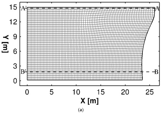
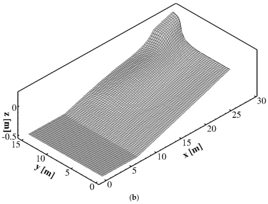
Figure 1.
(a): Plan view of the curvilinear computational grid (Only one out of every five coordinate lines is shown). (b): three-dimensional view of the bottom.
In Figure 2 we compare, along the two cross-sections, the wave heights obtained by the proposed model with the experimental results of Hamm [29]. From this figure, a good agreement can be noticed between the experimental and numerical results, for both the section placed in the sloping beach and the one placed in the rip channel.
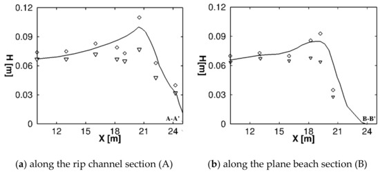
Figure 2.
Wave height comparison between the numerical results (solid line) obtained with the proposed model and the experimental data (diamonds represent the experimental data for significant wave height and gradients represent the experimental data for variance-based wave height ) from Hamm [29]
The wave induced nearshore current obtained by the proposed model is shown in Figure 3, where only one out of every four time-averaged (over 120 wave periods) flow velocity vectors is visualised. As can be seen in Figure 3, the differences in the wave elevation between the plane beach and rip channel drives an alongshore current that turns offshore producing the rip current at the rip channel position. This circulation pattern can be considered erosive, since it can produce a dragging of the sediments towards the offshore region.
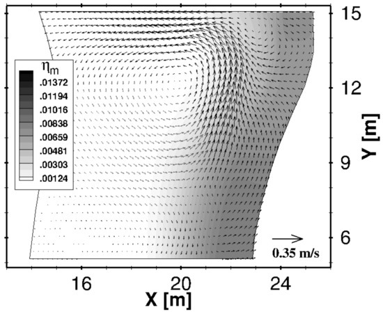
Figure 3.
Plan view detail of the time averaged (over 120 wave periods) velocity field. Only one out of every four vectors is shown.
3.2. The Effects of a System of Submerged Breakwaters in a Coastal Area with a Curvilinear Shoreline
The submerged breakwaters are among the most common works realised for the protection of the coastlines affected by erosion phenomena of different intensities. A group of submerged breakwaters separated by gaps protects the coastline against the erosive action of the wave motion as it induces the wave breaking. The energy associated with the incident wave motion is partially reflected offshore and partially dissipated by breaking over the barriers, thus weakening the erosional power of the waves passing over the breakwaters. Furthermore, submerged breakwaters separated by gaps are designed in such a way as to induce, immediately downstream of the breakwaters, gradients of the mean water level, producing circulation patterns that induce bottom accretion (accretive conditions) [30,31]. As experimentally demonstrated [32,33], the distance between the breakwaters and the coastline or the depth of the submerged breakwaters with respect to the undisturbed free surface level are parameters which must be chosen in such a way to favour the development of accretive circulations near the coastline, rather than erosive ones.
Figure 4 shows a schematisation of the hydrodynamic effects produced by a system of submerged breakwaters on the mean water level: Figure 4a refers to a cross-section in correspondence with the barriers; Figure 4b refers to a cross-section along the gap between the barriers. As shows in Figure 4a, close to the submerged breakwaters, due to the wave breaking there is an increase in the mean water level with respect to the still water level (wave set-up ). On the onshore side of the breakwater, the wave breaking stops because the waves enter the relatively deeper waters in the lee of the breakwater, then the wave (which is now characterised by a new height) restarts to shoal until it breaks near the coastline. At the coastline, the total set-up with respect to the still water level is given by the sum of the two successive wave set-ups (). As schematised in Figure 4b, between the barriers, the incident waves propagate without being directly affected by the presence of the barriers and break near the shoreline. Consequently, in the gap between the barriers, the waves set-up is lower than the one () that takes place over the barriers (). This difference in the mean water level drives a rip current in the gap that is directed offshore. Furthermore, in the protected area between the barriers and the shoreline, the modifications produced on the incident waves by the presence of the barriers induce nearshore circulations which can be summarised in two different circulation pattern types.
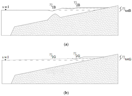
Figure 4.
Schematic cross-section and profile of the set-up; (a) section placed over the submerged breakwater (b) section placed in the gap between the barriers.
The first type is characterised by the fact that, near the shoreline, the mean water level in correspondence with the section placed between the barriers is higher than the one in correspondence with the section placed over the barriers (). This induces a secondary circulation with direction opposite the primary one and thus induces an accumulation of suspended sediments in the sheltered area and the advancement of the shoreline (accretive conditions). This type of circulation pattern is known as four-cell circulation (Figure 5a).
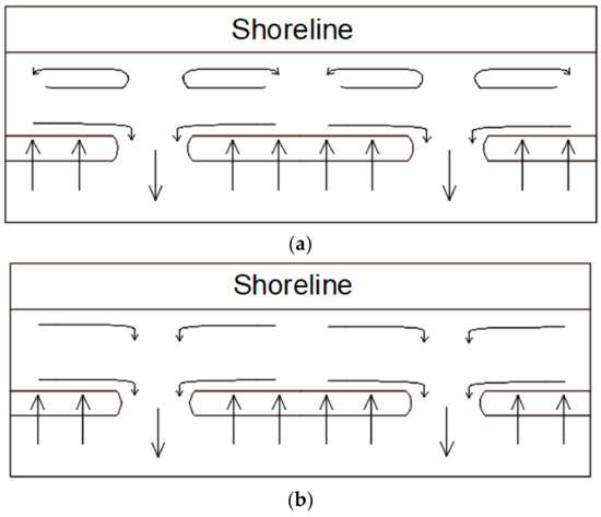
Figure 5.
(a) Accretive circulation pattern (b) Erosive circulation pattern.
The second type is characterised by the fact that, near the shoreline, the mean water level in correspondence with the section between the barriers is lower than the one in correspondence with the section placed over the barriers (). This induces a secondary circulation with the same direction as the primary one. This type of circulation pattern is known as two-cell circulation (Figure 5b). The two-cell circulation produces a dragging of the sediments towards the offshore region, thus favouring the erosion of the seabed at the coastline with possible shoreline regression (erosive conditions).
From a general point of view, in order to obtain accretive conditions, a system of submerged breakwaters separated by gaps has to produce a partial decrease of wave energy and wave height in the lee of the barriers such that the waves transmitted break closer to the shoreline than those at the gaps and with a smaller wave set-up . As shown by Ranasinghe et al. [30,31], for given wave characteristics (wave height and period), the main factors of a system of submerged breakwaters separated by gaps that can cause erosive or accretive conditions are: the water depth at the bar crest, ; the ratio between the length of the barrier and the gap width, ; the distance from shoreline to barrier, . All other factors being equal, as the water depth at the bar crest decreases, the wave height reduction of the transmitted waves increases. It can produce a wave set-up, , lower than the one produced by the waves passing through the gaps, (accretive conditions). Concerning the ratio between the length of the barrier and the gap width, , all other factors being equal, a reduction of increased the amount of water accumulated in the sheltered area. Consequently, near the shoreline, the wave set-up induced by the transmitted waves can be greater than the one produced by the waves passing through the gaps, (erosive conditions). On the contrary, as the distance from shoreline to barrier increases, all other factors being equal, the distance between the first and second wave breaking enhances, thus reducing the amount of water accumulated in the sheltered area. It can produce a wave set-up, , lower than the one in correspondence of the gaps, , (accretive conditions).
In this section, we verify whether the presence of a submerged coastal defence structure in the coastal area with curvilinear shoreline described in the previous section, is able to modify the wave induced circulation pattern and the hydrodynamic conditions from erosive to accretive. The coastal defence structure is made up of two submerged breakwaters, separated by a gap, similar to the ones used in the experimental test shown in Section 3.1: the barrier length is 3.6 m, the distance between the barriers is 1.8 m, and the average water depth at the bar crest is 2.67 cm. We use the same curvilinear computational grid as in the previous test and numerically simulate two different cases: in Case 1 the submerged breakwaters are positioned inside the surf-zone at an average distance from the shoreline (calculated from the crest of the barrier) that is approximatively 2 m whereas in Case 2, the same system of barriers is positioned at the beginning of the surf-zone, at an average distance from the shoreline that is approximatively 4 m.
3.3.1. Case 1
Figure 6a shows the bathymetry in presence of the two submerged breakwaters for the Case 1. A three-dimensional view of the bottom of the curvilinear computational grid is shown in Figure 6b. Figure 6c–d shows two significant cross-sections: one in the gap between the barriers () and another over the barrier (). The incident wave conditions are the same as the previous test: wave period and wave height .
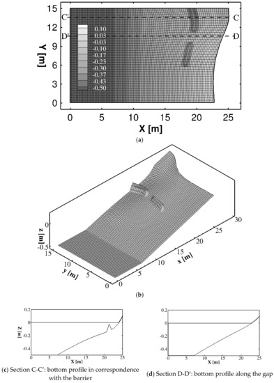
Figure 6.
Case 1: (a): Plan view of the curvilinear computational grid (Only one out of every five coordinate lines is shown). (b): three-dimensional view of the bottom. (c–d): bottom profiles in section C-C’ and D-D’.
Figure 7 shows a three-dimensional detail of an instantaneous wave field, in which the nearshore currents are fully developed. The figure shows that the presence of the barriers partially influences the coastal hydrodynamics: the waves that break over the barriers undergo a small reduction in the wave height with respect to those that propagate on the plane beach.
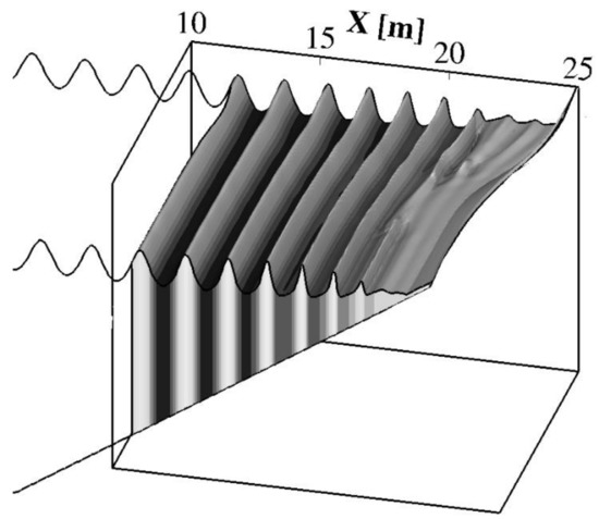
Figure 7.
Case 1: Three-dimensional view detail of an instantaneous wave field at the time when the breaking induced circulation is fully developed.
This difference in the wave height is shown in Figure 8a, where the wave height evolution along the two above mentioned sections is presented. Figure 8b shows the time-average (over 120 wave periods) of the cross-shore velocity components calculated near the bottom along the section in the gap between the barriers (section D-D’). In this figure, positive values represent offshore directed velocities.
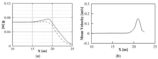
Figure 8.
Case 1: (a) Wave height comparison between section C-C’ (solid line) and section D-D’ (dashed line); (b) Time-averaged (over 120 wave periods) cross-shore velocity component along the section in the gap between the barriers (section D-D’).
Figure 9 shows a plan view of the time-averaged (over 120 wave periods) velocity field near the bottom in which the nearshore currents are fully developed. From this figure it is possible to notice the presence of a circulation pattern characterised by flow velocities that, in the entire lee zone, are directed from the centreline of the barrier to the gaps, where they return offshore. In fact, close to the shoreline, the wave set-up in the gaps is lower than the one in the lee of the barrier; this gradient in the mean water level drives diverging currents that characterise the above mentioned two-cell erosive circulation pattern. In this Case 1, the presence of the barriers does not significantly alter the surf-zone dynamics and consequently is not able to modify the hydrodynamic conditions from erosive to accretive.
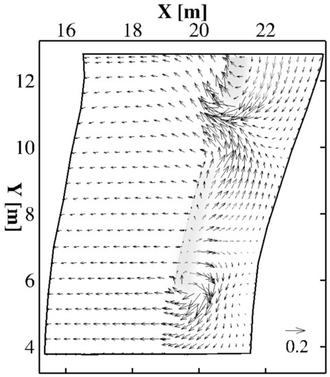
Figure 9.
Case 1: Plan view detail of the time averaged (over 120 wave periods) velocity field. Only one out of every four vectors is shown.
3.3.2. Case 2
Figure 10a shows the bathymetry in the presence of the two submerged breakwaters for Case 2. A three-dimensional view of the bottom of the curvilinear computational grid is shown in Figure 10b. Figure 10c–d shows two significant cross sections: one in the gap between the barriers () and another over the barrier (). The incident wave conditions are the same as the previous case. From Figure 10 it can be noticed that breakwaters are approximatively 2 m more offshore than Case 1.
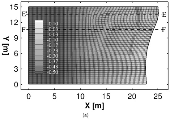
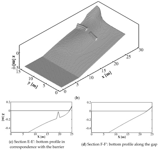
Figure 10.
Case 2: (a): Plan view of the curvilinear computational grid (Only one out of every five coordinate lines is shown). (b): three-dimensional view of the bottom. (c–d): bottom profiles in section C-C’ and D-D’.
Figure 11 shows a three-dimensional detail of an instantaneous wave field in which the nearshore currents are fully developed. The figure shows that, in this case, the presence of the barriers greatly influences the coastal hydrodynamics: the waves that break over the barriers undergo a significant reduction with respect to those that propagate on the plane beach—the wave that propagates in the gap between the barriers undergoes an increase in the wave height due to the presence of a rip current directed offshore.
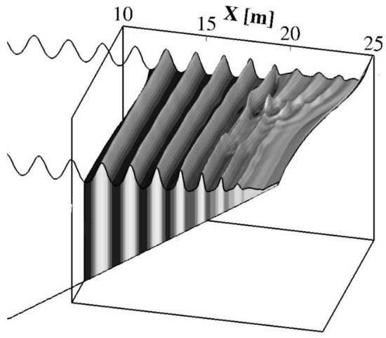
Figure 11.
Case 2 Three-dimensional view detail of an instantaneous wave field at the time when the breaking induced circulation is fully developed.
This difference in the wave height is shown in Figure 12a where the wave height evolution along the two above mentioned sections is presented. Figure 12b shows the time-averaged (over 120 wave periods) cross-shore velocity component calculated near the bottom along the section in the gap between the barriers (section F-F’). With respect to Case 1, the significant reduction in the wave height produced by the breakwaters induces a rip current significantly greater than in Case 1.
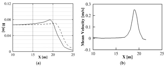
Figure 12.
Case 2: (a) Wave height comparison between section E-E’ (solid line) and section F-F’ (dashed line); (b) Time-averaged cross-shore (over 120 wave periods) velocity component along the section in the gap between the barriers (section F-F’).
Figure 13 shows the vertical time-averaged cross-shore (over 120 wave periods) velocity component respectively at and . As can be observed in Figure 13, the vertical structure of the mean horizontal flow under breaking waves is characterised by onshore directed velocities near the free surface and offshore directed velocities near the bottom (undertow). From these figures, it is possible to deduce that the proposed three-dimensional non-hydrostatic numerical model is able to represent the three-dimensional circulation that occurs, on the offshore side (Figure 13a) and onshore side (Figure 13b) of the submerged breakwater.
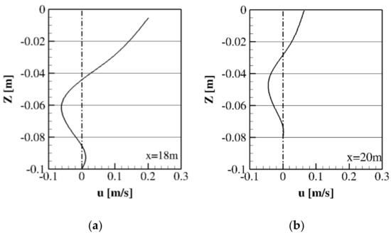
Figure 13.
Case 2: Vertical time-averaged (over 120 wave periods) cross-shore velocity profile (a) (b)
Figure 14 shows a plan view of the time-averaged (over 120 wave periods) velocity field near the bottom in which the nearshore currents are fully developed. From this figure, it is possible to notice the presence of a primary circulation characterised by onshore directed flow velocities over the barrier that return offshore at the gaps. In the same figure a secondary circulation it can be seen, opposite the primary one, that takes place near the shoreline. In fact, close to the shoreline, the wave set-up in the gaps is greater than the one in the lee of the barrier—this gradient in the mean water level drives converging currents that characterise the above mentioned four-cell accretive circulation pattern.
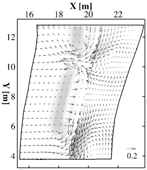
Figure 14.
Case 2: Plan view detail of the time averaged (over 120 wave periods) velocity field. Only one out of every four vectors is shown.
4. Conclusions
A three-dimensional numerical study of the hydrodynamic effects produced by a system of submerged breakwaters in a coastal area with a curvilinear shoreline has been proposed. The three-dimensional numerical model adopted in this paper is based on the integral contravariant formulation of the Navier-Stokes equations in a time-dependent curvilinear coordinate system proposed in [25]. The flow velocity fields and free surface elevation produced by the wave propagation over a system of submerged breakwaters separated by gaps have been simulated. The numerical results show that, for given wave conditions, the positioning of submerged breakwaters in the surf zone induced nearshore currents that can favour the sedimentation of the sediment in the lee of the barriers (accretive circulation pattern). On the contrary, for the same wave conditions, the positioning of the submerged breakwaters too close to the shoreline is not able to modify the circulation pattern from erosive to accretive.
Author Contributions
Conceptualization and methodology F.G. and G.C.; investigation F.P.
Funding
This research received no external funding.
Conflicts of Interest
The authors declare no conflict of interest.
References
- Van der Meer, J.W.; Briganti, R.; Zanuttigh, B.; Wang, B. Wave transmission and reflection at low-crested structures: Design formulae, oblique wave attack and spectral change. Coast. Eng. 2005, 52, 915–929. [Google Scholar] [CrossRef]
- Williams, H.E.; Briganti, R.; Romano, A.; Dodd, N. Experimental analysis of wave overtopping: A new small scale laboratory dataset for the assessment of uncertainty for smooth sloped and vertical coastal structures. J. Mar. Sci. Eng. 2019, 7, 217. [Google Scholar] [CrossRef]
- Van Doorslaer, K.; Romano, A.; De Rouck, J.; Kortenhaus, A. Impacts on a storm wall caused by non-breaking waves overtopping a smooth dike slope. Coast. Eng. 2017, 120, 93–111. [Google Scholar] [CrossRef]
- Romano, A.; Bellotti, G.; Briganti, R.; Franco, L. Uncertainties in the physical modelling of the wave overtopping over a rubble mound breakwater: The role of the seeding number and of the test duration. Coast. Eng. 2015, 103, 15–21. [Google Scholar] [CrossRef]
- Franco, L.; Geeraerts, J.; Briganti, R.; Willems, M.; Bellotti, G.; De Rouck, J. Prototype measurements and small-scale model tests of wave overtopping at shallow rubble-mound breakwaters: The Ostia-Rome yacht harbour case. Coast. Eng. 2009, 56, 154–165. [Google Scholar] [CrossRef]
- Cannata, G.; Lasaponara, F.; Gallerano, F. Non-linear Shallow Water Equations numerical integration on curvilinear boundary-conforming grids. WSEAS Trans. Fluid Mech. 2015, 10, 13–25. [Google Scholar]
- Cannata, G.; Petrelli, C.; Barsi, L.; Fratello, F.; Gallerano, F. A dam-break flood simulation model in curvilinear coordinates. WSEAS Trans. Fluid Mech. 2018, 13, 60–70. [Google Scholar]
- Lorenzoni, C.; Postacchini, M.; Brocchini, M.; Mancinelli, A. Experimental study of the short-term efficiency of different breakwater configurations on beach protection. J. Ocean Eng. Mar. Energy 2016, 2, 195–210. [Google Scholar] [CrossRef]
- Postacchini, M.; Russo, A.; Carniel, S.; Brocchini, M. Assessing the Hydro-Morphodynamic response of a beach protected by detached, impermeable, submerged breakwaters: A numerical approach. J. Coast. Res. 2016, 32, 590–602. [Google Scholar]
- Hsiao, S.C.; Liu, P.L.-F.; Hwung, H.H.; Woo, S.B. Nonlinear water waves over a three-dimensional porous bottom using Boussinesq-type model. Coast. Eng. J. 2005, 47, 231–253. [Google Scholar] [CrossRef]
- Pelinovsky, E.; Choi, B.H.; Talipova, T.; Woo, S.B.; Kim, D.C. Solitary wave transformation on the underwater step: Asymptotictheory and numerical experiments. Appl. Math. Comput. 2010, 217, 1704–1718. [Google Scholar] [CrossRef]
- Peregrine, D.H. Long waves on a beach. J. Fluid Mech. 1967, 27, 815–827. [Google Scholar] [CrossRef]
- Wei, G.; Kirby, J.T.; Grilli, S.T.; Subramanya, R. A fully nonlinear Boussinesq model for surface waves. Part 1. highly nonlinear unsteady waves. J. Fluid Mech. 1995, 294, 71–92. [Google Scholar] [CrossRef]
- Chen, Q.; Kirby, J.T.; Dalrymple, R.A.; Shi, F.; Thornton, E.B. Boussinesq modeling of longshore currents. J. Geophys. Res. 2003, 108, 26-1–26-18. [Google Scholar] [CrossRef]
- Gallerano, F.; Cannata, G.; De Gaudenzi, O.; Scarpone, S. Modeling bed evolution using weakly coupled phase-resolving wave model and wave-averaged sediment transport model. Coast. Eng. J. 2016, 58, 1650011-1–1650011-50. [Google Scholar] [CrossRef]
- Roeber, V.; Cheung, K.F. Boussinesq-type model for energetic breaking waves in fringing reef environments. Coast. Eng. 2012, 70, 1–20. [Google Scholar] [CrossRef]
- Tatlock, B.; Briganti, R.; Musumeci, R.E.; Brocchini, M. An assessment of the roller approach for wave breaking in a hybrid finite-volume finite-difference Boussinesq-type model for the surf-zone. Appl. Ocean Res. 2018, 73, 160–178. [Google Scholar] [CrossRef]
- Lin, P.; Li, C.W. A σ-coordinate three-dimensional numerical model for surface wave propagation. Int. J. Numer. Methods Fluids 2002, 38, 1045–1068. [Google Scholar] [CrossRef]
- Young, C.C.; Wu, C.H. A σ-coordinate non-hydrostatic model with embedded Boussinesq-type-like equations for modeling deep-water waves. Int. J. Numer. Methods Fluids 2010, 63, 1448–1470. [Google Scholar] [CrossRef]
- Cannata, G.; Petrelli, C.; Barsi, L.; Camilli, F.; Gallerano, F. 3D free surface flow simulations based on the integral form of the equations of motion. WSEAS Trans. Fluid Mech. 2017, 12, 166–175. [Google Scholar]
- Gallerano, F.; Cannata, G.; Lasaponara, F.; Petrelli, C. A new three-dimensional finite-volume non-hydrostatic shock-capturing model for free surface flow. J. Hydrodyn. 2017, 29, 552–566. [Google Scholar] [CrossRef]
- Bradford, S.F. Non-hydrostatic model for surf zone simulation. J. Waterw. Port Coast. Ocean Eng. 2011, 137, 163–174. [Google Scholar] [CrossRef]
- Ma, G.; Shi, F.; Kirby, J.T. Shock-capturing non-hydrostatic model for fully dispersive surface wave processes. Ocean Model. 2012, 43–44, 22–35. [Google Scholar] [CrossRef]
- Cannata, G.; Gallerano, F.; Palleschi, F.; Petrelli, C.; Barsi, L. Three-dimensional numerical simulation of the velocity fields induced by submerged breakwaters. Int. J. Mech. 2019, 13, 1–14. [Google Scholar]
- Cannata, G.; Petrelli, C.; Barsi, L.; Gallerano, F. Numerical integration of the contravariant integral form of the Navier–Stokes equations in time-dependent curvilinear coordinate systems for three-dimensional free surface flows. Contin. Mech. Thermodyn. 2019, 31, 491–519. [Google Scholar] [CrossRef]
- Palleschi, F.; Iele, B.; Gallerano, F. Integral contravariant form of the Navier-Stokes equations. WSEAS Trans. Fluid Mech. 2019, 14, 101–113. [Google Scholar]
- Luo, H.; Bewley, T.R. On the contravariant form of the Navier-Stokes equations in time-dependent curvilinear coordinate systems. J. Comput. Phys. 2004, 199, 355–375. [Google Scholar] [CrossRef]
- Aris, R. Vectors, Tensors, and the Basic Equations of Fluid Mechanics; Dover Publications: New York, NY, USA, 1989. [Google Scholar]
- Hamm, L. Directional nearshore wave propagation over a rip channel: An experiment. In Proceedings of the 23rd International Conference of Coastal Engineering, Venice, Italy, 4–9 October 1992; pp. 226–239. [Google Scholar]
- Ranasinghe, R.; Turner, I.L. Shoreline response to submerged structures: A review. Coast. Eng. 2006, 53, 65–79. [Google Scholar] [CrossRef]
- Ranasinghe, R.; Larson, M.; Savioli, J. Shoreline response to a single shore-parallel submerged breakwater. Coast. Eng. 2010, 57, 1006–1017. [Google Scholar] [CrossRef]
- Haller, M.C.; Dalrymple, R.A.; Svendsen, I.A. Experimental modeling of a rip current system. In Proceedings of the 1997 3rd International Symposium on Ocean Wave Measurement and Analysis, WAVES, Virginia Beach, VA, USA, 3–7 November 1997; pp. 750–764. [Google Scholar]
- Haller, M.C.; Dalrymple, R.A.; Svendsen, Ib.A. Experimental study of nearshore dynamics on a barred beach with rip channels. J. Geophysical Res. 2002, 107, 14-1–14-21. [Google Scholar] [CrossRef]


© 2019 by the authors. Licensee MDPI, Basel, Switzerland. This article is an open access article distributed under the terms and conditions of the Creative Commons Attribution (CC BY) license (http://creativecommons.org/licenses/by/4.0/).