Article

Analysis of Slope Failure Behaviour Based on Real-Time Measurement Using the x–MR Method

1
Citizens Safety Division, Yongin City, Gyeonggi-do 17019, Korea
2
Department of Regional Infrastructure Engineering, Kangwon National University, Chuncheon 24341, Korea
*
Author to whom correspondence should be addressed.
J. Mar. Sci. Eng. 2019, 7(10), 360; https://doi.org/10.3390/jmse7100360
Submission received: 7 August 2019 / Revised: 1 September 2019 / Accepted: 30 September 2019 / Published: 10 October 2019

Abstract

:
A real-scale slope failure model experiment is performed to analyze the movement behavior of the slope during failure, and the results are analyzed through the x–MR control chart method, along with inverse displacement and various analysis sections such as K-values. As a result, the portent of failure can be identified to be about 7.7–18.3 min prior to the final slope failure. As a result of the analyses of changes in the control limit in the various analyses sections, it is considered that the application of K = 3 to the x-MR control chart is effective. It is observed that using the x-MR control chart technique of the inverse displacement is useful for the early prediction of the anomalous behavior of a slope, through a more quick and objective judgment. Henceforth, it is necessary to establish clear techniques for prediction and analyses of slope failure through continuous research, and those results can be used as the basic data of a slope instrumentation management standard that can contribute to the mitigation of life and property damage caused by slope failure hazards.

1. Introduction

Economic losses and fatalities due to natural hazards, such as slope failure, have increased in number worldwide [1,2,3,4,5]. Recently, slope disasters, such as landslides and slope failures, caused by concentrated torrential rain and typhoons—due to climate change—have occurred in South Korea every year, resulting in massive damage to human life and property [6]. Since two-thirds of the total land in South Korea is mountainous areas, artificial development of the mountainous areas for industrialization and urbanization is inevitable. During this development process, stable slopes are destroyed, which then causes landslides. The scale of this damage also has been increasing simultaneously [7]. The instrumentation of landslide-prone slopes is essential to eventually issue early warning for landslides, to reduce casualties and property damage. To this end, designing a real-time sensing and safety investigation system through real-time monitoring is required. This requires the design and development of instruments and effective maintenance techniques for predicting slope movement and stability by applying various real-time instrumentation techniques [8].
Although many studies are underway to study procedures for reducing damage caused by landslides, it is still almost impossible to predict landslides [9], and there is yet no way to stop a slope from collapsing. Nevertheless, various studies on slope failure occurrence processes, landslide inducing factors, real-time monitoring, and landslide warning systems have contributed to the technical basis of early warning systems [10,11,12,13,14]. Lari et al. [15] proposed a probabilistic approach by expressing a landslide hazard as a function of landslide destructive power, which considers the displacement rate rather than the magnitude. Haneberg [16], Park et al. [17], Raia et al. [18], Lee and Park [19], and Zhang et al. [20] used the Monte Carlo (MC) simulation and treated soil properties in regional-scale applications using a probabilistic approach by selecting random variables from a given probability density function (PDF). Salciarini et al. [21] considered geostatistical methods for the spatial distribution of soil properties to enhance preceding approaches and used the point estimate method (PEM), which was computationally a more efficient method than an MC simulation. These probabilistic approaches were not aimed explicitly at spatial real-time early warning systems, however.
Working in South Korea, many academic and government-affiliated research institutes constantly have been studying landslide-related instrumentation techniques through the design of scientific management systems, such as the design of a real-time monitoring system in landslide-prone steep slopes. Since there are still few studies on the prediction of landslides through analyses of ground movement, by not predicting a landslide-prone area, research on analytical methods that can precisely predict landslide occurrence is paramount to mitigate casualties and economic losses due to landslides [22,23].
The control chart theory, first proposed by Shewhart [24], is an effective theory that statistically controls the variation in the process over time. It has been used as an essential tool for quality control in manufacturing processes and, recently, has been used widely throughout the slope instrumentation management industry, such as in the design of monitoring systems, sensors, etc. [25].
Particularly, in the field of slope instrumentation, Yoo [26] analyzed the utility of statistical control chart techniques by analyzing the measured data of real-time slope failure warning systems, through automated instrumentation systems, using the statistical analysis method (probabilistic analysis method) and the mathematical analysis method (deterministic analysis method). Kwon et al. [25] obtained hourly displacement data from the ground displacement instrumentation system, analyzed them using various statistical control techniques, and developed a slope instrumentation data analysis system based on these data analyses.
Additionally, Yoo et al. [27] emphasized the necessity to design a safety inspection system and develop control techniques to comprehend the occurrence of unexpected situations and ground movement in the landslide-prone slopes. Furthermore, he determined the possibility of slope failure prediction through statistical control techniques for real-time data obtained from surface displacement sensors for this purpose. Kim et al. [28] proposed a statistical analysis method that can analyze variation in the landslide-inducing factors, due to rainfall in the model slope, and reviewed the applicability of the early warning system by setting the management standard using the obtained analyses result.
Therefore, in this study, slope failure model tests are conducted through construction and cutting of the real-scale model slopes. The ground movement characteristics are assessed through a statistical control technique, using displacement data obtained from the experiment, which is of great significance in terms of instrumentation and maintenance of landslide-prone slopes.

2. x–MR Control Chart

The x–MR control chart technique, proposed by Shewhart [24], is a statistical management method for analyzing the state and maintaining the stability of the target control object for uniformity in quality. Since the calculation is relatively easy, and its application range is wide, it is used widely for process and quality control [29].
A control chart is a type of statistical quality control technique which is used to inspect and maintain the stability state of a process. It is a statistical method that can maintain the process in a controlled state by use of quality characteristics that indicate the state of the process, provide instant identification of the reasons for quality fluctuation, and take measures to solve the problems. The control chart is a statistical technique, in other words, which is able to set statistical control limit lines, upper, and lower control lines that can make rational decisions at both the top and bottom portions to determine dispersion caused by coincidence or anomaly. It is able to detect instantaneously the cause of an anomaly or coincidence during the process and promptly can detect the dispersion due to coincidence and anomaly by plotting the quality characteristic values (measured values, data) that represent the state of the process. The control chart in Figure 1 consists of the measured value, centerline, control limit line, etc. The control limit line is a criterion for deciding the anomalous state of the measured values.
Figure 1 shows a schematic diagram of the statistical control method, in which the data obtained from the control target object is on the Y-axis and time is on the X-axis. The control chart is symmetric about the mean μ and the degree of dispersion σ, where μ is the mean of the normally distributed data and σ is the standard deviation [30].
Here, the basic concept of the control chart is to evaluate quality control by using the probabilistic method for μ and σ. The control limits, viz. UCL (Upper Control Limit) and LCL (Lower Control Limit), of ±3σ are set with respect to the centerline and, when a point deviates beyond the control limit lines, the data obtained from the process is decided to be an anomaly condition [31].
The control limit line is a baseline that is set for making simple decisions regarding the anomaly condition and the probability distribution of data to be within the range of μ − 3σ ≤ x ≤ μ + 3σ is approximately 99.73%.
The x–MR control chart, used in this study, is a method to analyze the individual control chart (x) that represents individual data of the measured values and the moving range (MR) control chart simultaneously. Seen in Figure 2, the analysis interval (K), upon which the control limit depends, is set. Then, the moving range (MR), indicating the difference between the maximum value (xmax) and the minimum value (xmin) within the interval, is marked on the control chart.

3. Real Scale Slope Failure Simulation

3.1. Real Scale Slope Construction for Slope Failure Simulation

During this study, the displacement data obtained from the cutting process on a real scale model slope were analyzed using an x–MR control chart. The field experiments were performed three times for the reliability of the experimental data. The model slope construction processes of the real scale slope failure simulation are discussed in the following paragraphs.
Soil samples for the model experiment were obtained from natural slopes located in Chuncheon city. Weathered soil is a type of soil formed by weathering of parent rocks due to various causes. It is evenly distributed throughout South Korea and it is considered to be suitable to depict characteristics of the general slope.
The weathered soil, used in this study, was classified as SW according to the Unified Soil Classification System (USCS), therefore, the particle size distribution was well-graded sand, had a dry density ( ρ d ) of 17.58 kN/m3 and fines content of 11.4% (refer to Table 1). The optimum water content (wopt), obtained through a TP (Test Pit, in-situ density test) and compaction tests, was used during construction so the constructed model slope resembled the ground surface conditions.
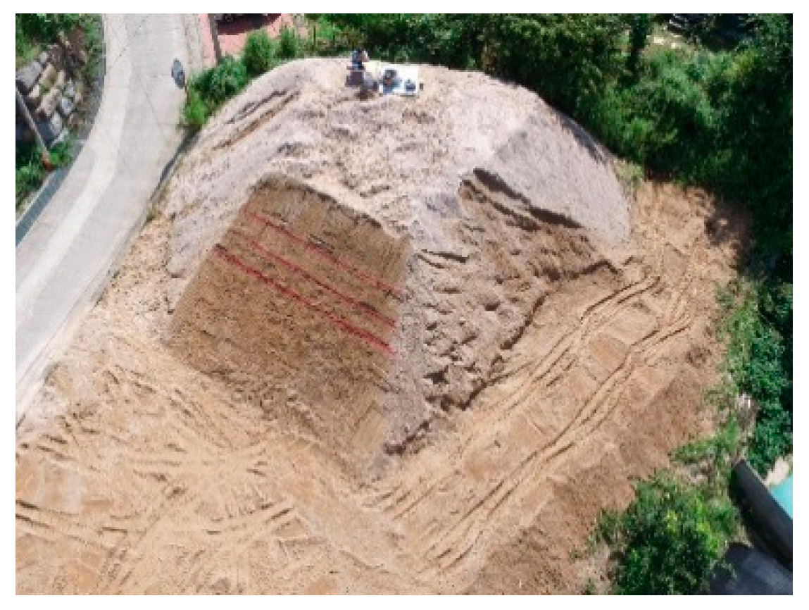
The model slope reflects the results of the preliminary study through numerical analysis (limit equilibrium analysis). The cross-section of the model slope, as in Figure 3, had a 5.0 m height, and the cutting processes were carried out in three steps. During the model slope construction process, the soil was deposited under free-fall conditions using the bucket of a backhoe to depict deposition and sedimentation of soil due to weathering effects. Lastly, no additional load, such as compaction, was applied to the upper portion of the slope so the prevailing slope conditions could be depicted in which only the self-weight of the soil acts. (refer to Figure 4). Subsequent to completing construction of the model slope, cutting sections (step 1–step 3) were labeled according to the slope cutting plan.

3.2. Slope Failure Simulation by Slope Cutting

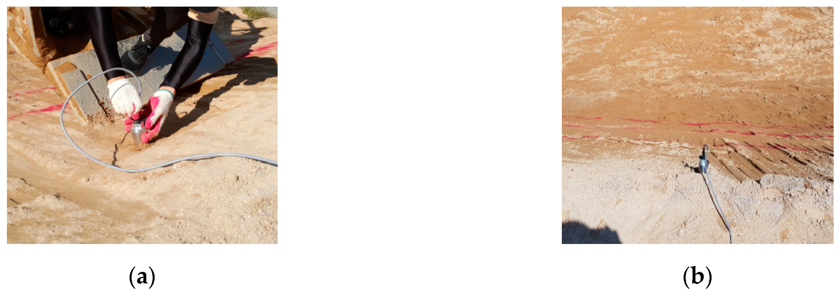
During this study, the slope behavior, (slope failure), was simulated artificially by cutting the soil mass from the toe of the model slope in a stepwise manner so the cutting edge was vertical. To inspect the slope movement, subsurface strain gauges were installed at a position 50 cm apart (refer to Figure 5). The subsurface strain gauge, used in this study, was in the form of a pipe with a diameter of 10 mm and consisting of a strain sensor attached at the central part of the pipe, which was capable of sensing the bending deformation occurring in the pipe during the slope movement. The strain sensors were connected to the data logger, where the measured data were automatically saved at an interval of one second.
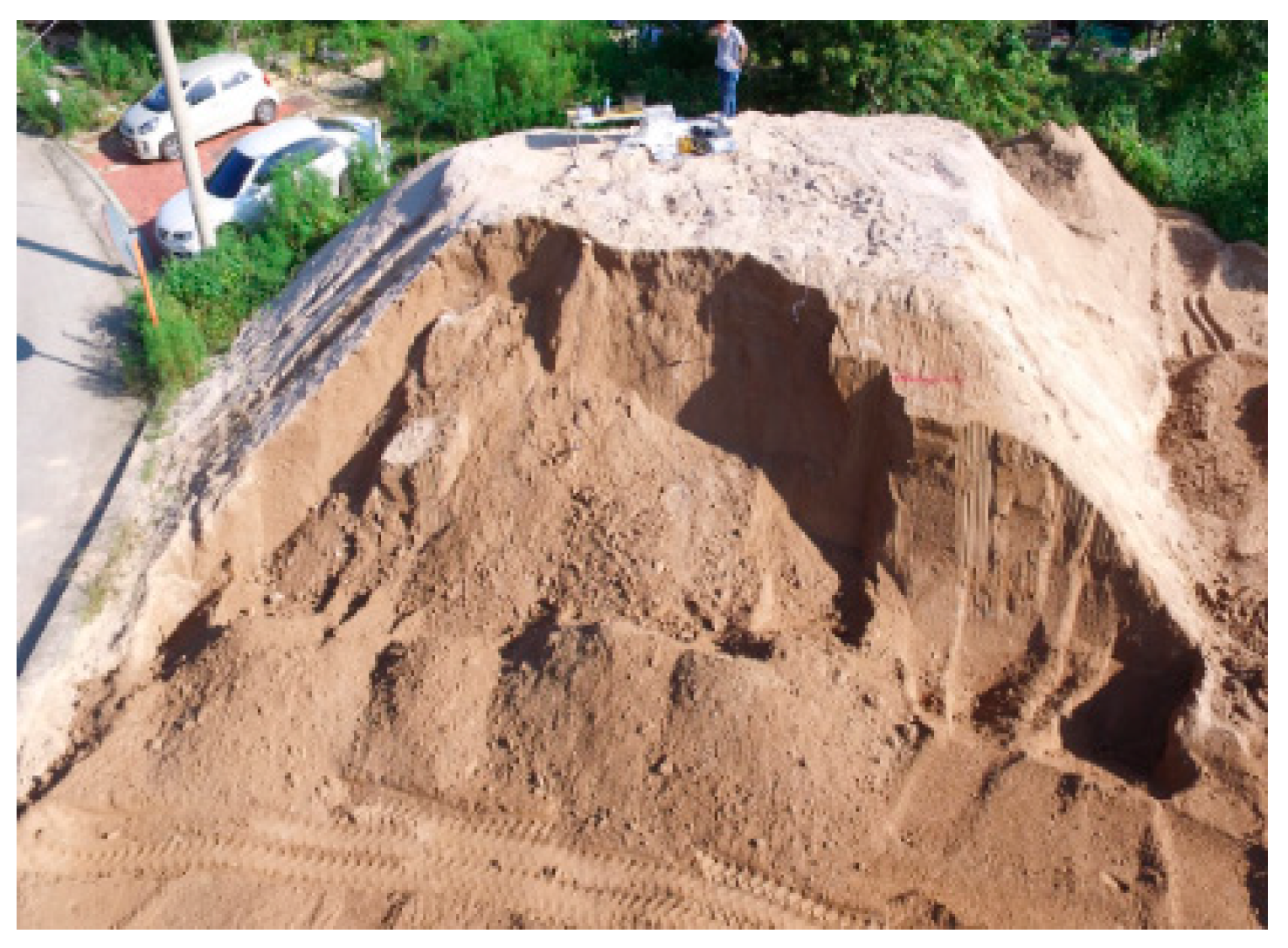
Artificial cutting of the model slope surface using a backhoe is shown in Figure 6, and the slope failure that occurred after the cutting is shown in Figure 7.
During the stepwise cutting process, cutting was carried out according to the planned section, maintaining waiting time. A total time of 20 min, cutting and waiting time combined, was applied and the same backhoe was used during slope construction and the cutting process.

4. Analysis of Experimental Results

4.1. Analysis of the Behaviour of Slope Failure

Considering all three cases, we could confirm the failure point by comparing the obtained data and the experimental results. Figure 8 shows the ground displacement characteristics for each case of the slope cutting (Supplementary Materials).
In case 1, the onset of a small ground displacement until 13 min, a uniform increase in displacement until 38 min, and a rapid displacement rate until 43 min after the start of the experiment were observed. Thereafter, the rate of increase of displacement was reduced somewhat, and the slope failure finally occurred at about 49.5 min after the start of the experiment.
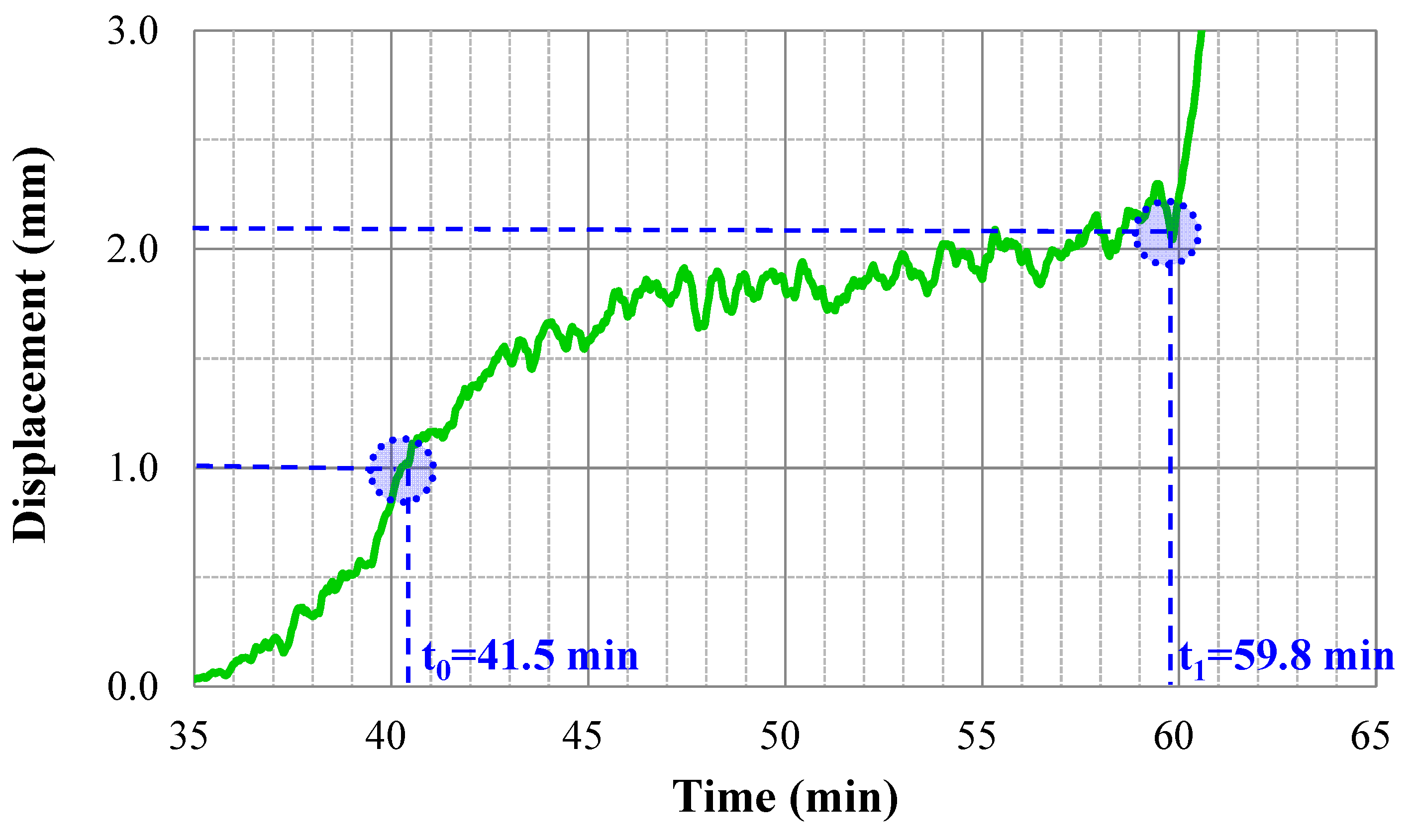
Case 2 showed irregular movement continuously from the start of the experiment and sudden failure occurred at about 35.0 min. The displacement rate was accelerated rapidly up to about 43.0 min, and since then, there was no progress in ground movement. Finally, the slope failure occurred at about 59.8 min of elapsed time.
Seen in case 3, the ground motion was not observed from the outset of the experiment, but slight motion was monitored at about 14.0 min, and the constant increase rate of displacement was monitored until about 48 min. The displacement rate accelerated rapidly up to about 52.0 min. Thereafter, gradual displacement continued, and sudden failure occurred at about 54.7 min.
Continuous ground displacement was monitored from the outset of the experiment to the final slope failure, which indicates progressive slope failure in all cases.
The Japanese Steep Slope Measurement Control Criterion, which is frequently used in local practice, suggests that the management standard value of the maintenance phase is more than 1 mm/day (Ministry of Public Safety and Security (2016)). Therefore, the value of the acquired data that was less than 1 mm was considered to be abnormal and, also, an insignificant signal caused, due to electrical noise, was not used for the analysis.
As a result, it can be verified that cases 1 and 2, showing a progressive failure tendency that included displacement of 1 mm or more, could detect the slope failure beforehand, whereas it can be concluded that prediction of slope failure was not possible in case 3.

4.2. x–MR Control Chart Analysis

During this study, the displacement data obtained from case 1 and case 2, in which prediction of slope failure was possible, were used to perform an x–MR control chart.
Regarding case 1, the data used in the x–MR control chart were displacement data of 7.7 min total time from 41.8 to 49.5 min, until the final collapse occurred (refer to Figure 9). Similarly, the measured data for a total time of 18.3 min, from 41.5–59.8 min, until the final collapse occurred was selected in case 2 (refer to Figure 10).
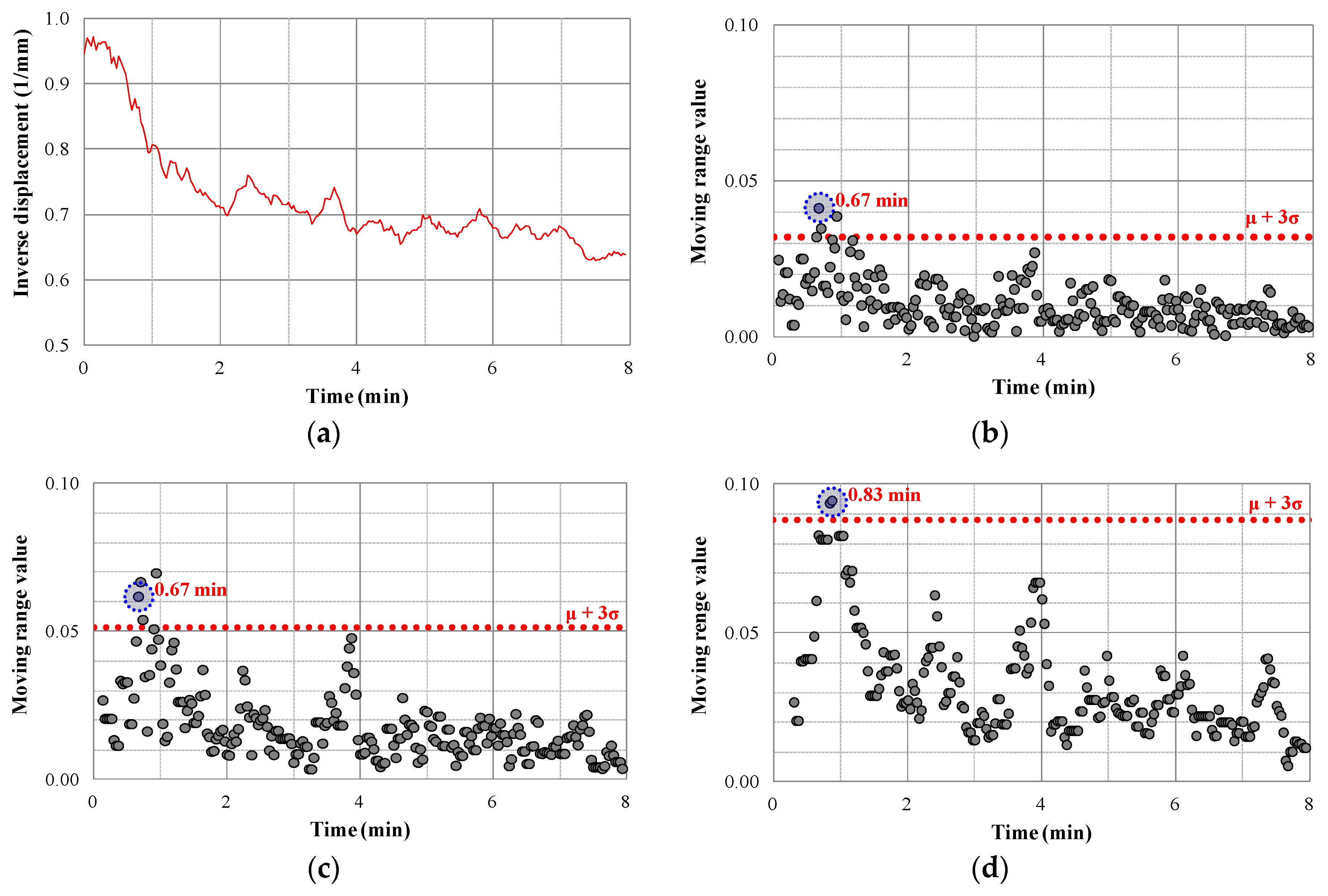
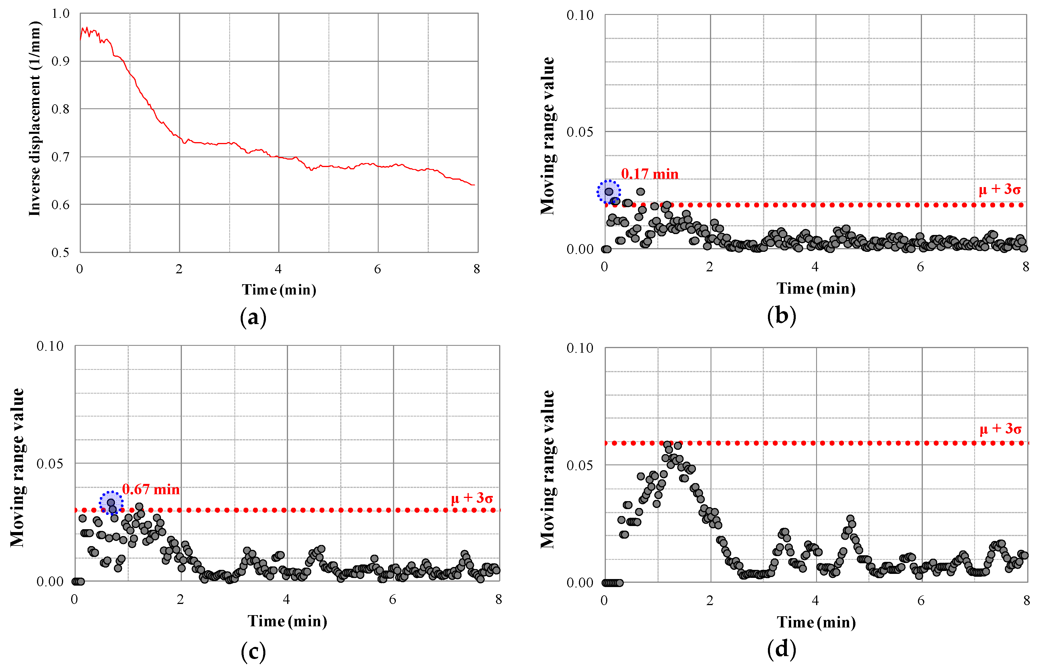
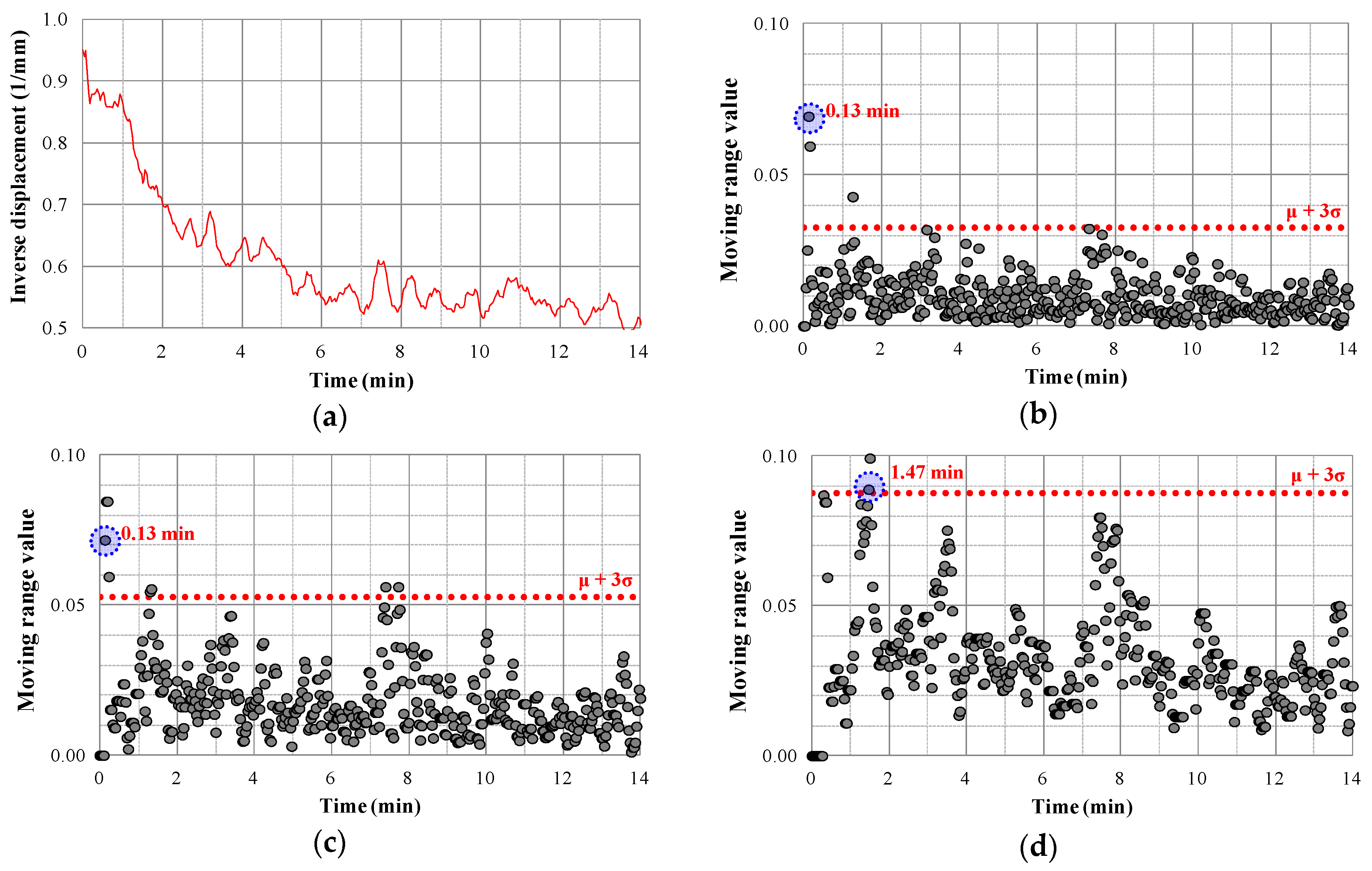
Voight [32] suggested a method of estimating the slope failure time using the slope displacement and displacement velocity data transformed into inverse form over time. Park et al. [33] obtained the ground displacement data through field model tests and analyzed slope movement characteristics by using inverse displacement over time. Fukuzono et. al. [34] observed the inverse rate of movement of the extensometer and proposed a method for predicting the time point of slope failure by using the variation of displacement over time. Tamate et. al. [35] used the method of Fukuzono et. al. [34] for predicting the slope failure by the use of shear strain rate. Thus, the reciprocal of displacement, (inverse displacement), has been used for the prediction of slope failure in this study. Figure 11 and Figure 12 and Figure 13 and Figure 14 show the x–MR control charts of time-varying inverse displacement and varying k-values using 10-points and 30-points moving average, for data from the start of the experiment to slope failure, for case 1 and case 2, respectively.
Considering all cases (excluding moving average = 30, K = 10 of case 1, refer to Figure 12d), the moving average is confirmed to exceed the μ + 3σ control limit from t0, time point from which significant displacement data were obtained, to t1, time point of the final failure. It is considered that the degree of risk of slope failure can be evaluated sufficiently depending on whether meaningful data is obtained or not.
When the anomalous state is analyzed for the interval excluding the moving average, it is confirmed that the risk can be evaluated after 0.10–0.67 min for K = 3, 0.05–0.67 min for K = 5, and 0.07–1.47 min for K = 10. Although the timing of risk assessment is not significantly different depending on the analysis interval, it is deemed reasonable to apply K = 3 considering the urgency of failure at the steep slope.
Since the analysis results of this study are obtained from two field experiments, it is expected to be able to be used in the evacuation management standard based on additional field experiments and slope failure case data, if a reliable moving average and analysis interval (K) can be selected.

4.3. Proposal for Slope Instrumentation Standards

Presently, there are lots of difficulties in applying a single ultimate standard for various field conditions in South Korea, thus the standard published in 1996 by the Commission of Slope Stability in Japan is being practiced still [36]. Although relevant standards and instrumentation management standards presented and proposed by various research and development projects in the field of slope failure suggest an analysis of displacement rate and maximum (cumulative) displacement, it is infeasible to apply these values in the actual field. Therefore, in this study, a slope instrumentation standard is suggested through the analysis of the results using a statistical control chart technique.
Generally, a slope management standard is a method of recognizing the slope behavior by the amount of displacement and issuing early warning of slope failure by analyzing the actual movement. During this study, we tried to set a standard for evacuation management in steep slope failure by studying the criteria for prediction of steep slope failure and analyzing the displacement data measured for steep slope failure cases.
The slope instrumentation standard is classified into a total of three categories. The displacement section of less than 1mm, which has an insignificant value, is the normal phase, the displacement section of more than 1mm is the anomalous phase, and then the slope failure phase (refer to Table 2). The normal phase is deemed to be safe through the control chart analysis, the anomalous phase is deemed to be unsafe, and the time of progression from the anomalous phase to the slope failure phase is found to be about 7.7–18.3 min. Since the failure phase is a crucial situation, evacuation of local residents near the slope should be completed before the failure phase is reached.
Since the evacuation of local residents should proceed within 7.7–18.3 min after the risk detection, it is necessary to establish a strategy to induce evacuation of local residents through temporal and spatial considerations, as well as determine the propagation method of this information. The slope instrumentation standard, proposed in this study, is based on the analysis of limited experimental data, however. Although the limitation is distinct, the reliability of the evacuation management standard can be improved through continuous experiments, and numerical analysis, which easily can consider various slope conditions.

5. Conclusions

During this study, real scale slope failure simulation experiments were performed to analyze the movement characteristics during slope failure and the results were analyzed through the x–MR control charts based on inverse displacement and K values. The conclusions of this study are as follows:
(1)
As a result of the real scale slope failure model test, the final slope failure was confirmed in all the cases. However, the slope failure was predictable in cases 1 and 2 beforehand, in which the progressive failure that included displacement exceeding 1 mm was observed. However, in case 3, the pre-prediction was not possible prior to the slope failure.
(2)
Based on evaluation of the slope failure for various moving ranges (K) through an x–MR control chart on significant displacement data, it is concluded that applying K = 3 is effective.
(3)
The x–MR control approach of inverse displacement can be applied to make quick and objective decisions about slope failure behavior and for predicting slope failure.
(4)
It is considered that the analysis method of slope failure proposed through this study can increase the efficiency of the disaster management policy implementation for local government officials by providing more reliable risk assessment results, along with the steep slope failure prediction, early warning system, landslide information system, etc.
Henceforth, it is necessary to establish clear techniques for prediction and analysis of slope failure through continuous research. Those results can be used as the basic data for a slope measurement management standard, which can contribute to mitigation of life and property damage caused by the slope failure hazards.

Supplementary Materials

The following are available online at https://www.mdpi.com/2077-1312/7/10/360/s1.

Author Contributions

Conceptualization, Y.K.; Data curation, S.P., B.T. and J.J.; Formal analysis, S.P. and Y.K.; Funding acquisition, Y.K.; Investigation, Y.K.; Methodology, S.P. and B.T.; Project administration, Y.K.; Resources, B.T., J.J., S.L. and S.C.; Software, S.P., H.L., J.J., S.L. and S.C.; Supervision, Y.K.; Validation, S.P., H.L. and Y.K.; Writing—original draft, H.L.; Writing—review & editing, B.T. and S.L.

Funding

This work was supported by Korea Institute of Planning and Evaluation for Technology in Food, Agriculture, Forestry and Fisheries (IPET).

Acknowledgments

This work was supported by Korea Institute of Planning and Evaluation for Technology in Food, Agriculture, Forestry and Fisheries (IPET) through Advanced Production Technology Development Program, funded by Ministry of Agriculture, Food and Rural Affairs (MAFRA) (116114-03).

Conflicts of Interest

The authors declare no conflicts of interest.

References

  1. Barredo, J.I. Normalised flood losses in Europe: 1970–2006. Nat. Hazards Earth Syst. Sci. 2009, 9, 97–104. [Google Scholar] [CrossRef]
  2. European Environment Agency. Mapping the Impacts of Natural Hazards and Technological Accidents in Europe. An Overview of the Last Decade; European Environment Agency: København, Denmark, 2010; ISBN 9789292131685. [Google Scholar]
  3. EM-DAT. The OFDA/CRED International Disaster Database; Université Catholique de Louvain: Brussels, Belgium; Available online: http://www.emdat.be/ (accessed on 6 August 2019).
  4. Alfieri, L.; Salamon, P.; Pappenberger, F.; Wetterhall, F.; Thielen, J. Operational early warning systems for water-related hazards in Europe. Environ. Sci. Policy 2012, 21, 35–49. [Google Scholar] [CrossRef]
  5. Piciullo, L.; Calvello, M.; Cepeda, J.M. Territorial early warning systems for rainfall-induced landslides. Earth-Sci. Rev. 2018, 179, 228–247. [Google Scholar] [CrossRef]
  6. Eun-Chul, S.; Kim, J.-I. Stability Analysis of Geocell Reinforced Slope During Rainfall. J. Korean Geosynth. Soc. 2017, 16, 33–41. [Google Scholar]
  7. Han, J.-G.; Hong, K.-K.; Lee, J.-Y.; Jung, S.-K. Application Evaluation of Countermeasure Method using Analysis of Failure Causes for Reinforced Slope. J. Korean Geosynth. Soc. 2011, 10, 9–18. [Google Scholar]
  8. Korea Institute of Geoscience and Mineral Resources. Development of an Integrated Early Detection System of Landslides Based on a Real-Time Monitoring; Research Institute Report: Gyeonggi-do, Korea, 2014. (In Korean) [Google Scholar]
  9. Wieczorek, G.; Snyder, J. Monitoring slope movements. Geol. Monit. 2009, 245–271. Available online: http://www.science.earthjay.com/instruction/chemeketa/2015_spring/GEO144/lectures/lecture_07/GEO144_lecture_7_Wieczorek_Snyder_2009_overview_monitoring_slope_movements.pdf (accessed on 2 July 2019).
  10. Keefer, D.K.; Wilson, R.C.; Mark, R.K.; Brabb, E.E.; Brown, W.M.; Ellen, S.D.; Harp, E.L.; Weiczorek, G.F.; Alger, C.S.; Zazkin, R.S. Real-Time Landslide Warning During Hearvy Rainfall. Science 1987, 238, 921–925. [Google Scholar] [CrossRef]
  11. Wilson, R.C. The Rise and Fall of a Debris-Flow Warning System for the San Francisco Bay Region, California. In Landslide Hazard and Risk; John Wiley & Sons: Hoboken, NJ, USA, 2012; pp. 493–516. ISBN 9780471486633. [Google Scholar]
  12. Godt, J.W.; Baum, R.L.; Chleborad, A.F. Rainfall characteristics for shallow landsliding in Seattle, Washington, USA. Earth Surf. Process. Landf. 2006, 31, 97–110. [Google Scholar] [CrossRef]
  13. Chleborad, A.F.; Baum, R.L.; Godt, J.W.; Powers, P.S. A prototype system for forecasting landslides in the Seattle, Washington, area. GSA Rev. Eng. Geol. 2008, 20, 103–120. [Google Scholar]
  14. Baum, R.L.; Godt, J.W. Early warning of rainfall-induced shallow landslides and debris flows in the USA. Landslides 2010, 7, 259–272. [Google Scholar] [CrossRef]
  15. Lari, S.; Frattini, P.; Crosta, G.B. A probabilistic approach for landslide hazard analysis. Eng. Geol. 2014, 182, 3–14. [Google Scholar] [CrossRef] [Green Version]
  16. Haneberg, W.C. A rational probabilistic method for spatially distributed landslide hazard assessment. Environ. Eng. Geosci. 2004, 10, 27–43. [Google Scholar] [CrossRef]
  17. Park, H.J.; Lee, J.H.; Woo, I. Assessment of rainfall-induced shallow landslide susceptibility using a GIS-based probabilistic approach. Eng. Geol. 2013, 161, 1–15. [Google Scholar] [CrossRef]
  18. Raia, S.; Alvioli, M.; Rossi, M.; Baum, R.L.; Godt, J.W.; Guzzetti, F. Improving predictive power of physically based rainfall-induced shallow landslide models: A probabilistic approach. Geosci. Model Dev. 2014, 7, 495–514. [Google Scholar] [CrossRef]
  19. Lee, J.H.; Park, H.J. Assessment of shallow landslide susceptibility using the transient infiltration flow model and GIS-based probabilistic approach. Landslides 2016, 13, 885–903. [Google Scholar] [CrossRef]
  20. Zhang, S.; Zhao, L.; Delgado-Tellez, R.; Bao, H. A physics-based probabilistic forecasting model for rainfall-induced shallow landslides at regional scale. Nat. Hazards Earth Syst. Sci. 2018, 18, 969–982. [Google Scholar] [CrossRef] [Green Version]
  21. Salciarini, D.; Fanelli, G.; Tamagnini, C. A probabilistic model for rainfall—Induced shallow landslide prediction at the regional scale. Landslides 2017, 14, 1731–1746. [Google Scholar] [CrossRef]
  22. Park, S.; Min, Y.; Kang, M.; Jung, H.; Sami, G.; Kim, Y. Slope Failure Prediction through the Analysis of Surface Ground Deformation on Field Model Experiment. J. Korean Geosynth. Soc. 2017, 16, 1–10. [Google Scholar]
  23. Sung-yong, P.; Hee-don, J.; Young-ju, K.; Yong-seong, K. A study on Behavior of Slope Failure Using Field Excavation Experiment. J. Korean Soc. Agric. Eng. 2017, 59, 101–108. (In Korean) [Google Scholar]
  24. Shewhart, W.A. Some Applications of Statistical Methods to the Analysis of Physical and Engineering Data. Bell Syst. Tech. J. 1924, 3, 43–87. [Google Scholar] [CrossRef]
  25. Kwon, O.; Baek, Y.; Seo, Y.S. Development of slope displacement data analysis system using control chart theory. In Proceedings of the Conference of the Korean Society of Engineering Geology, Cheongju, Korea, 6–7 November 2008; pp. 137–143. [Google Scholar]
  26. Yoo, B. A Study of Failure Analysis Methods Based on Real-Time Monitoring Data for Landslide Warning System. Ph.D. Dissertation, Graduate School Kumoh National Institute of Technology, Gumi, Korea, 2006. (In Korean). [Google Scholar]
  27. Yoo, B.S.; Park, Y.D.; Lee, K.S.; Chang, K.T. Failure Prediction and Analysis of Prone-landslide with x-MR Control Chart. In Proceedings of the 35th Korean Society of Civil Engineers Conference, Gangwon-do, Korea, 21–23 October 2009; Volume 10, pp. 1779–1802. (In Korean). [Google Scholar]
  28. Kim, S.B. Unstable Soil Behavior Detecting Methods in Flume Test Using Applied Statistical Analysis; Chungbuk National University: Cheongju, Korea, 2014. (In Korean) [Google Scholar]
  29. Koutras, M.V.; Bersimis, S.; Maravelakis, P.E. Statistical process control using shewhart control charts with supplementary runs rules. Methodol. Comput. Appl. Probab. 2007, 9, 207–224. [Google Scholar] [CrossRef]
  30. Yun, H.S.; Song, K.K.; Shin, Y.W.; Kim, C.Y.; Choo, S.Y.; Seo, S.S. Application of x-MR control chart on monitoring displacement for prediction of abnormal ground behaviour in tunnelling. J. Korean Tunn. Undergr. Space Assoc. 2014, 16, 445–458. [Google Scholar] [CrossRef]
  31. Yim, S.; Seo, Y.-S. A New Method for the Analysis of Measured Displacements during Tunnelling using Control Charts. J. Eng. Geol. 2009, 19, 261–268. [Google Scholar]
  32. Voight, B. A method for prediction of volcanic eruptions. Nature 1988, 332, 125–130. [Google Scholar] [CrossRef]
  33. Park, S.; Chang, D. Prediction of Slope Failure Using Control Chart Method. J. Korean Geosynth. Soc. 2018, 17, 9–18. [Google Scholar]
  34. Fukuzono, T. A Method to Predict the Time of Slope Failure Caused by Rainfall Using the Inverse Number of Velocity of Surface Displacement. Landslides 1985, 22, 8–13. [Google Scholar] [CrossRef]
  35. Tamate, S.; Hori, T.; Mikuni, C.; Suemasa, N. Experimental analyses on detection of potential risk of slope failure by monitoring of shear strain in the shallow section. In Proceedings of the 18th International Conference on Soil Mechanics and Geotechnical Engineering, Paris, France, 2–6 September 2013; pp. 1901–1904. [Google Scholar]
  36. Lee, J.D. The R&D Research on Construction of Monitoring Management System for Evacuation Inhabitant in Steep Slope Site and Development of Monitoring Specification; Disaster and Safety Management Institute: Sejong-si, Korea , May 2015. (In Korean) [Google Scholar]
Figure 1. A Schematic Diagram of x–MR Control Chart Method.
Jmse 07 00360 g001
Figure 2. x–MR control chart; (a) Calculation of Rxi at i = 1 (b) Calculation of Rxi at i = 2.
Jmse 07 00360 g002
Figure 3. Cross-section diagram of the model slope.
Jmse 07 00360 g003
Figure 4. Construction of the model slope.
Jmse 07 00360 g004
Figure 5. Installation of a sensor: (a) Penetration of the sensor into the model slope; (b) Connection of the sensor through a wire.
Jmse 07 00360 g005
Figure 6. Slope cutting by a backhoe.
Jmse 07 00360 g006
Figure 7. Slope failure after cutting.
Jmse 07 00360 g007
Figure 8. Displacement over time during slope cutting experiment of the model slope.
Jmse 07 00360 g008
Figure 9. Displacements from 41.8 to 49.5 min (case 1).
Jmse 07 00360 g009
Figure 10. Displacements from 41.5 to 59.8 min (case 2).
Jmse 07 00360 g010
Figure 11. x–MR control chart method for displacement data of case 1 (moving average = 10 points): (a) Inverse displacement data (moving average = 10 points); (b) Moving range (K = 3); (c) Moving range (K = 5); (d) Moving range (K = 10).
Jmse 07 00360 g011
Figure 12. x–MR control chart method for displacement data of case 1 (moving average = 30 points): (a) Inverse displacement (moving average = 30 points); (b) Moving range (K = 3); (c) Moving range (K = 5); (d) Moving range (K = 10).
Jmse 07 00360 g012
Figure 13. x–MR control chart method for displacement data of case 2 (moving average = 10 points): (a) Inverse displacement (moving average = 10 points); (b) Moving range (K = 3); (c) Moving range (K = 5); (d) Moving range (K = 10).
Jmse 07 00360 g013
Figure 14. x–MR control chart for displacement data of case 2 (moving average = 30 points): (a) Inverse displacement (moving average = 30 points); (b) Moving range (K = 3); (c) Moving range (K = 5); (d) Moving range (K = 10).
Jmse 07 00360 g014
Table 1. Properties of the weathered soil used in the study.
USCS ρ d (kN/m3) ρ d m a x (kN/m3)wopt (%)Sand (%)Silt (%)Clay (%)D50 (mm)
SW17.5818.8913.356.19.81.60.85
Table 2. Slope instrumentation management standard.
StepDisplacement (s) (mm)Time (t0) (min)Control LimitPhase
10 < s < 1.0-SafeNormal Phase
21.0 < s < 1.50.1UnsafeAnomalous Phase
3s > 1.5 7.7-Failure Phase