A Model for Intact and Damage Stability Evaluation of CNG Ships during the Concept Design Stage

Abstract

To face the design of a new ship concept, the evaluation of multiple feasible solutions concerning several aspects of naval architecture and marine engineering is necessary. Compressed natural gas technologies are in continuous development; therefore, there are no available databases for existing ships to use as a basis for the design process of a new unit. In this sense, the adoption of a modern multi-attribute decision-based method can help the designer for the study of a completely new ship prototype. A database of compressed natural gas ships was generated starting from a baseline hull, varying six hull-form parameters by means of the design of experiment technique. Between the attributes involved in the concept design process, stability is for sure one of the most relevant topics, both for intact and damaged cases. This work describes two approaches to identify the compliance of a ship with the intact stability regulations based on the ship main geometrical quantities. Moreover, a metamodel based on the maximum floodable length concept (damage stability) allows determining the main internal subdivision of the ship. The metamodel outcomes were compared with results from direct calculations on a ship external to the database, highlighting the adequate accuracy given by the developed methods.

1. Introduction

The design process of a ship is a complex issue that faces many aspects of naval architecture and marine engineering, varying from hull-form development to ship’s production. Among the phases of the ship design, the concept one is of utmost importance. In fact, through this design stage, the main decisions have to be taken that will influence the whole ship design process and also techno-economic success of the ship in its lifetime. It is therefore necessary to adopt a modern design approach starting from the first feasibility studies, involving multi-attribute decision-making (MADM) strategies [1]. To this end, it should be possible to evaluate the ship’s primary attributes through mathematical metamodels in terms of the ship’s main geometrical parameters. This fact is even more crucial in the case of a completely new ship prototype such as a Compressed Natural Gas (CNG) ship [2]. The continuous technological improvement in the pressure vessel containment systems makes the CNG ship design even more complicated. The existing CNG ships have been designed and built with outdated pressure vessel technologies that led to the design of high block coefficient ($C_B$) units with a low economical design speed [3,4]. Explorative studies highlight that adoption of a modern and lighter containment system would lead to more slender ships sailing at higher speeds [5]. However, no indication is given on how the new types of pressure vessels (PV) would influence the definition of new CNG ship concepts. Therefore, no database of existing CNG ships is available for the generation of the metamodels needed for a robust MADM design process. Thus, it is essential to build a ship’s database starting from a baseline ship. The database is the starting point for the development of the metamodels. In the present study, the focus was on ship stability requirements, being these among the most important attributes to evaluate from the concept design stage. In the literature, simple models can be found to estimate critical values for the vertical centre of gravity position [6]. Here, intact stability requirements were considered to build a metamodel suitable to predict quickly and accurately the stability characteristics of a large number of ships during a MADM process by means of multiple linear regression (MLR) technique directly on the righting arm curves. To this end, multiple options have been tested and compared with each other. Besides, working on the same database, a model to determine also damage stability issues has been developed, adopting the maximum floodable length concept and allowing to evaluate preliminary subdivision. In this paper, the methods adopted to develop the metamodels for intact and damage stability are described, together with the determination of the database. Finally, to evaluate the reliability of the proposed method, a comparison is provided between the developed models and direct calculations on a ship external from the database.

2. CNG Ships

Natural gas is the most environmentally-friendly solution, among hydrocarbons sources, for energy production. Therefore, it is reasonable to suppose that natural gas production will grow in the next decades, requiring more flexibility for resource exploitation [7]. To this end, marine transportation of the natural gas also will have a higher impact on the market [8]. Between the possible technologies for natural gas transportation at sea, compressed natural gas technology is starting to be economically attractive for marine transportation of natural gas for long-medium distances and large gas volumes [9,10]. The CNG solution is attractive because it does not require the presence of costly on-shore infrastructures such as liquefaction and regasification plants, but only two single mooring points for loading and offloading [11]. CNG is then a flexible option for gas transportation, which is giving even more importance to the ship design. Specifically, due to the continuous improvements in the PV’s materials and technologies, the ship design process has to deal with totally new units without any existing reference.

Because of the absence of existing comparable designs, some assumptions have to be made concerning the kind of CNG ship that is desired to be analysed. As mentioned, the technologies used for the PV influence greatly the CNG ship design. Modern technologies combining composites and steel structures or using composite only, allow reducing the weight of the containment system, leading to more slender hull forms compared to first CNG ship prototypes [12]. Another distinctive characteristic of CNG units is the presence of a flat bottom part in the bow to allow the connection of the submerged turret loading (STL) for the gas loading operation [13]. The selection of the propulsion system is also changing the ship shape, as highlighted in a previous study comparing twin-skeg solution with single-skeg ones [14].

Independently of the shape of the vessel or the propulsion choice, a CNG ship has to fulfil a dedicated set of regulations. This study focused on the intact and damage stability requirements that are hereafter described in detail.

2.1. Intact Stability Requirements

During the ship design, the stability of a ship shall fulfil the rules issued by international bodies. The stability criteria have to be met in different loading conditions in order to assure a minimum level of safety. Therefore, during the concept design, these criteria are essential to select, among all possible design alternatives, only the feasible ones, rejecting all the generated solutions where at least one criterion is not satisfied. The CNG ships’ intact stability is subject to Intact Stability Code (ISC) [15], which states well-known requirements on the metacentric height, on the righting arm curve $GZ$ shape, and on the ship’s dynamic stability. In detail, the following criteria shall be met regarding $GZ$ shape:

I1.

The area under $GZ$ curve up to 30 deg shall be at least 0.055 m rad.

I2.

The area under $GZ$ curve up to $min({\varphi }_f,40\mathrm{deg})$ shall be at least 0.090 m rad.

I3.

The area under $GZ$ curve from 30 deg to $min({\varphi }_f,40\mathrm{deg})$ shall be at least 0.030 m rad.

I4.

The righting lever $GZ$ shall be at least 0.2 m at an angle of heel equal to or greater than 30 deg.

I5.

The maximum righting lever shall occur at an angle of heel not less than 25 deg.

Here, ${\varphi }_f$ is the downflooding angle. Moreover, the metacentric height shall be at least 0.15 m, but this criterion was never proven to be critical for CNG ships; therefore, in this work, it is not considered. Finally, the weather criterion requirements shall be met. In detail, considering a ship subject to a steady wind heeling lever $l_{w1}$, rolling due to waves to an angle ${\varphi }_1$ and subject to a wind gust heeling lever $l_{w2}=1.5l_{w1}$, the following criteria shall be met:

W1.

The equilibrium angle under the effect of $l_{w1}$ should not exceed $min(0.8{\varphi }_{ds},16\mathrm{deg})$.

W2.

With reference to Figure 1, the area b shall be equal to or greater than area a.

Here, ${\varphi }_{ds}$ is the angle at deck submersion, ${\varphi }_2=min({\varphi }_f,{\varphi }_c,50\mathrm{deg})$ and ${\varphi }_c$ is the angle which vanish positive stability under the $l_{w2}$ heeling lever.

Therefore, to directly check the intact stability criteria, the $GZ$ curve and the area under the $GZ$ curve have to be estimated with sufficient accuracy since the concept design phase. It is worth noticing that, in such a phase, the hull forms are not defined in order to rapidly test multiple design alternatives while taking under control the computational load. Hence, metamodels based on statistics have to be adopted.

2.2. Damage Stability Requirements

Concerning damage stability, the problem is even more complex. CNG ships are subject to International Gas Code (IGC) [16], which defines the subdivision standards and the damaged stability criteria. In addition to this document, the class societies [17,18] also issued special requirements for CNG ships, which in some cases are even more conservative compared to IGC. All these rules have an impact on the ship subdivision, requiring in the cargo holds area a double bottom and a double hull: 760 mm for ABS, and $min(B/15,2\mathrm{m})$ for DNV-GL. Moreover, they define a minimum distance among subsequent PVs’ rows and between vessels and bulkheads/sides. Finally, a cofferdam is required between two cargo holds and between cargo holds areas and the other spaces. Namely, for each bulkhead, an entire row of pressure vessels is lost, leading to a reduction of ship capacity due to the watertight subdivision.

Besides, the IGC states that the ship, subject to the standard damages (

Table 1. Standard damage definition according to IGC code.

Damage Type	Extent (m)
	Longitudinal	Transverse	Vertical
Side	$min\left(\frac{1}{3}{L}^{2/3},14.5\right)$	$min\left(\frac{1}{5}B,11.5\right)$	no limitations
Bottom (x < 0.7 L)	$min\left(\frac{1}{3}{L}^{2/3},14.5\right)$	$min\left(\frac{1}{6}B,5.0\right)$	$min\left(\frac{1}{15}B,2.0\right)$
Bottom (elsewhere)	$min\left(\frac{1}{3}{L}^{2/3},14.5\right)$	$min\left(\frac{1}{6}B,10.0\right)$	$min\left(\frac{1}{15}B,2.0\right)$

) applied elsewhere or to any smaller damage with more severe consequences, is capable of surviving with sufficient residual stability. In detail, the following requirements shall be met at the final stage of flooding:

D1.

The $GZ$ curve shall have a minimum positive range of 20 deg.

D2.

The maximum residual lever within the 20 deg positive range shall be at least 0.1 m.

D3.

The area under $GZ$ curve within the 20 deg positive range shall be at least 0.0175 m rad.

The 20${}^{\circ }$ positive range can be measured from any angle commencing between the position equilibrium and the angle of 25${}^{\circ }$ or 30${}^{\circ }$ if the deck is not submerged. In addition, the rules the IGC code defines some requirements on the intermediate stages of flooding. Namely, it is required not to submerge any unprotected opening and not to exceed a 30${}^{\circ }$ heel angle. Furthermore, the residual stability at intermediate stages should not be significantly lower than the one required at the final stage. However, this last requirement is quite vague since it is not specified wha “significantly” means in terms of quantities. In the present study, only the criteria at final stage were taken into account.

In IGC code, it is also stated that a transversal bulkhead can be considered effective only if it has a distance from the contiguous ones greater than standard damage length. Hence, the cofferdams between cargo holds shall be neglected in damage stability calculations.

Thus, the CNG damaged stability requirements thus far described can be considered analogous to a deterministic rule with one/two subsequent flooded compartments. Therefore, to perform a preliminary allocation of the transverse bulkheads during concept design, it is possible to recover from SOLAS 90 the concept of floodable length adapting it to the current rule framework.

3. Materials and Methods

For the determination of a model suitable to predict the stability issues in the concept design stage, it is essential to find a method able to associate the stability attributes to the ship main dimensions. A database should be defined to obtain a design space in which the attributes can be determined. Specifically, the stability characteristics are related to the righting arm of the vessels. Therefore, for all the database individuals, the $GZ$ curves should be determined. It has been decided to reproduce the $GZ$ curves instead of the $KN$ curves for intact stability, in such a way to have inside the database the $KG$ variations necessary to evaluate a compact model for damage stability according to floodable lengths. On the obtained data, it is proposed to apply the MLR technique to identify a response surface suitable to predict the stability criteria in an early design stage, both in intact and in damage conditions.

3.1. Response Surface Methodology

In the engineering field, design of experiments (DOE) has been frequently used to reduce the number of experiments that need to be executed, resulting in a lower effort for experimentation and calculation work [19]. Response surface methodology (RSM) also quantifies the relationship between the controllable input parameters and the obtained response surface. The design procedure of RSM is as follows:

• Design a series of experiments for adequate and reliable measurement of the analysed response.
• Develop a mathematical model of the response surface with the best fitting.
• Represent the direct and interactive effects of process parameters through two- or three-dimensional plots.

Hereafter, the main steps of the procedure are described, starting from the database creation up to the definition of the mathematical models adopted for intact and damage stability cases.

3.1.1. CNG Ships Database

The first step needed for the creation of a mathematical metamodel is the creation of a database of ships. As mentioned, there is no available database of existing CNG ships. Then, it is necessary to create, starting from a baseline ship, a set of ships by systematically varying predetermined geometrical parameters submitted to given constraints. The constraints identify the design space for the investigation. The complexity of a ship leads to the possibility of changing many geometric parameters. These changes increase the number of individuals to generate inside the database to adequately cover the design space. To reduce the number of ships, some assumptions concerning the parameters and the methods that should be used to generate the database are mandatory. The main parameters to change for the study should be the ones having the highest impact on the ship attributes of interests. However, since the database is also oriented to be a basis for a complete study on the CNG ship type, the variations have to include also parameters needed to describe other relevant quantities for other ship’s attributes. In this sense, the main variables chosen for the database creation are $L/B$, $B/T$, $C_B$, $LCB$, $D/T$ and $KG/T$, where L is the ship length, B the ship breadth, T the ship design draught, $C_B$ the block coefficient, $LCB$ the longitudinal position of the centre of buoyancy (expressed in %L from midship, positive forward), D the ship depth and $KG$ the vertical position of the centre of gravity.

The first four parameters are general ones, related to the main dimensions and geometry of the hull-form, which can generally be used for the determination of other attributes linked with propulsion or motions [20]. $D/T$ and $KG/T$ are specific parameters for stability. All the variables vary between a minimum and a maximum, as reported in

Table 2. Design variables variation range.

Variable	${\mathit{C}}_{\mathit{B}}$	$\mathbf{LCB}$	$\mathit{L}/\mathit{B}$	$\mathit{B}/\mathit{T}$	$\mathit{D}/\mathit{T}$	$\mathbf{KG}/\mathit{T}$
ID	${\mathit{x}}_1$	${\mathit{x}}_2$	${\mathit{x}}_3$	${\mathit{x}}_4$	${\mathit{x}}_5$	${\mathit{x}}_6$
minimum	0.65	−3.00	6.0	4.0	2.0	1.5
medium	0.70	−2.25	6.5	4.5	3.0	2.0
maximum	0.75	−1.50	7.0	5.0	4.0	2.5

. The ranges were selected based on of previous studies [11,12,13,14], where specific ranges of geometrical coefficients were identified for the development of other metamodels (e.g., seakeeping, station-keeping, propulsion and internal layout). To maintain compliance with the other models, the same ranges were applied for the common variables. The specific stability variables ranges ($D/T$ and $KG/T$) were selected to investigate all the possible feasible solutions.

To optimise the number of individuals necessary to adequately describe the database, design of experiment techniques can be adopted [21]. For the selected case, a central composite face centred (CCF) space has been chosen, varying the seven design variables. This solution provide designs for the vertices and centre of the faces of an hypercube [22,23]. This choice allows covering the space between the extreme values of the variables, giving the possibility to fit regressions valid in almost all the internal space of the design hypercube. By selecting three levels for each variable, it is then possible to fit a quadratic model for the regressions; that means considering all the variables combinations up to the second order. Based on this scheme, for the database construction, a total of 45 ships was reproduced.

Table 3. CNG ships main characteristics.

	Non-Dimensional Variables						Main Dimensions
Ship ID	${\mathit{C}}_{\mathit{B}}$	$\mathbf{LCB}$	$\mathit{L}/\mathit{B}$	$\mathit{B}/\mathit{T}$	$\mathit{D}/\mathit{T}$	$\mathbf{KG}/\mathit{T}$	∇	$\mathbf{LCB}$	B	T	D	$\mathbf{KG}$
	-	$\%\mathit{L}$	-	-	-	-	m${}^3$	m	m	m	m	m
01	0.65	−3.00	6.0	4.0	2.0	1.5	36,111	94.00	33.33	8.33	16.67	12.50
02	0.65	−3.00	6.0	4.0	4.0	2.5	36,111	94.00	33.33	8.33	33.33	20.83
03	0.65	−3.00	6.0	5.0	2.0	2.5	28,889	94.00	33.33	6.67	13.33	16.67
04	0.65	−3.00	6.0	5.0	4.0	1.5	28,889	94.00	33.33	6.67	26.67	10.00
05	0.65	−3.00	7.0	4.0	2.0	2.5	26,531	94.00	28.57	7.14	14.29	17.86
06	0.65	−3.00	7.0	4.0	4.0	1.5	26,531	94.00	28.57	7.14	28.57	10.71
07	0.65	−3.00	7.0	5.0	2.0	1.5	21,224	94.00	28.57	5.71	11.43	8.57
08	0.65	−3.00	7.0	5.0	4.0	2.5	21,224	94.00	28.57	5.71	22.86	14.29
09	0.65	−1.50	6.0	4.0	2.0	2.5	36,111	97.00	33.33	8.33	16.67	20.83
10	0.65	−1.50	6.0	4.0	4.0	1.5	36,111	97.00	33.33	8.33	33.33	12.50
11	0.65	−1.50	6.0	5.0	2.0	1.5	28,889	97.00	33.33	6.67	13.33	10.00
12	0.65	−1.50	6.0	5.0	4.0	2.5	28,889	97.00	33.33	6.67	26.67	16.67
13	0.65	−1.50	7.0	4.0	2.0	1.5	26,531	97.00	28.57	7.14	14.29	10.71
14	0.65	−1.50	7.0	4.0	4.0	2.5	26,531	97.00	28.57	7.14	28.57	17.86
15	0.65	−1.50	7.0	5.0	2.0	2.5	21,224	97.00	28.57	5.71	11.43	14.29
16	0.65	−1.50	7.0	5.0	4.0	1.5	21,224	97.00	28.57	5.71	22.86	8.57
17	0.75	−3.00	6.0	4.0	2.0	2.5	41,667	94.00	33.33	8.33	16.67	20.83
18	0.75	−3.00	6.0	4.0	4.0	1.5	41,667	94.00	33.33	8.33	33.33	12.50
19	0.75	−3.00	6.0	5.0	2.0	1.5	33,333	94.00	33.33	6.67	13.33	10.00
20	0.75	−3.00	6.0	5.0	4.0	2.5	33,333	94.00	33.33	6.67	26.67	16.67
21	0.75	−3.00	7.0	4.0	2.0	1.5	30,612	94.00	28.57	7.14	14.29	10.71
22	0.75	−3.00	7.0	4.0	4.0	2.5	30,612	94.00	28.57	7.14	28.57	17.86
23	0.75	−3.00	7.0	5.0	2.0	2.5	24,490	94.00	28.57	5.71	11.43	14.29
24	0.75	−3.00	7.0	5.0	4.0	1.5	24,490	94.00	28.57	5.71	22.86	8.57
25	0.75	−1.50	6.0	4.0	2.0	1.5	41,667	97.00	33.33	8.33	16.67	12.50
26	0.75	−1.50	6.0	4.0	4.0	2.5	41,667	97.00	33.33	8.33	33.33	20.83
27	0.75	−1.50	6.0	5.0	2.0	2.5	33,333	97.00	33.33	6.67	13.33	16.67
28	0.75	−1.50	6.0	5.0	4.0	1.5	33,333	97.00	33.33	6.67	26.67	10.00
29	0.75	−1.50	7.0	4.0	2.0	2.5	30,612	97.00	28.57	7.14	14.29	17.86
30	0.75	−1.50	7.0	4.0	4.0	1.5	30,612	97.00	28.57	7.14	28.57	10.71
31	0.75	−1.50	7.0	5.0	2.0	1.5	24,490	97.00	28.57	5.71	11.43	8.57
32	0.75	−1.50	7.0	5.0	4.0	2.5	24,490	97.00	28.57	5.71	22.86	14.29
33	0.65	−2.25	6.5	4.5	3.0	2.0	27,350	95.50	30.77	6.84	20.51	13.68
34	0.75	−2.25	6.5	4.5	3.0	2.0	31,558	95.50	30.77	6.84	20.51	13.68
35	0.70	−3.00	6.5	4.5	3.0	2.0	29,454	94.00	30.77	6.84	20.51	13.68
36	0.70	−1.50	6.5	4.5	3.0	2.0	29,454	97.00	30.77	6.84	20.51	13.68
37	0.70	−2.25	6.0	4.5	3.0	2.0	34,568	95.50	33.33	7.41	22.22	14.81
38	0.70	−2.25	7.0	4.5	3.0	2.0	25,397	95.50	28.57	6.35	19.05	12.70
39	0.70	−2.25	6.5	4.0	3.0	2.0	33,136	95.50	30.77	7.69	23.08	15.38
40	0.70	−2.25	6.5	5.0	3.0	2.0	26,509	95.50	30.77	6.15	18.46	12.31
41	0.70	−2.25	6.5	4.5	2.0	2.0	29,454	95.50	30.77	6.84	13.68	13.68
42	0.70	−2.25	6.5	4.5	4.0	2.0	29,454	95.50	30.77	6.84	27.35	13.68
43	0.70	−2.25	6.5	4.5	3.0	1.5	29,454	95.50	30.77	6.84	20.51	10.26
44	0.70	−2.25	6.5	4.5	3.0	2.5	29,454	95.50	30.77	6.84	20.51	17.09
45	0.70	−2.25	6.5	4.5	3.0	2.0	29,454	95.50	30.77	6.84	20.51	13.68

collects the characteristics of each individual. The main dimensions of the ships were chosen to start from a baseline hull representative of the hypercube centre. All vessels were generated with a reference length of 200 m.

On the created database, dedicated calculations were performed using self developed codes [24] to determine the $GZ$ curves per each population member. Besides, per each ship, damage stability calculations have been performed, leading to the determination of the geometric floodable lengths $GFL$, checking the compliance with D1, D2 and D3 criteria. Some examples are given in Figure 2, reporting six hull-forms representing the principal variations inside the database together with the calculated $GZ$ and $GFL$ curves. It can be immediately noticed that the population includes also fully unstable ships having a fully negative $GZ$ curve, e.g. CNG 22. This is due to the combination between the geometrical variables and the $KG/T$, which, for some combinations, leads to negative $GM$ for the individual. It was selected to not discard these hulls, since the presence of unstable ships is necessary to determine the feasibility range of the design space. Thus, in a multi-criteria decision based design (DBD) process, the ships having parameters leading to a negative $GZ$ will be discarded from the selection process.

3.1.2. Multiple Linear Regressions

When all the considered variables of the problem can be considered as measurable, a response surface can be identified with the following expression:

$$y=f\left(x_1,x_2,x_3,\cdots ,x_n\right)$$

(1)

where y is the output of the system and $x_i$ are the n variables of action, also called factors. Under the assumption that the independent variables are continuous and controllable by experiments with negligible errors, a suitable approximation for the true functional relationship between independent variables and the response surface has to be found. Having used a CCF scheme for the database generation, it is possible to use a complete second-order model for the RSM, using the following general regression model:

$$y={\beta }_{r_{0,0}}+\sum _{i=1}^n{\beta }_{r_{i,0}}{x}_i+\sum _{i=1}^{n-1}\sum _{j=i+1}^n{\beta }_{r_{i,j}}{x}_i{x}_j+\sum _{i=1}^n{\beta }_{r_{i,i}}{x}_i^2+{\epsilon }_r$$

(2)

where ${\beta }_{r_{i,j}}$ are unknown parameters and ${\epsilon }_r$ is the regression error. There are several methods to evaluate the unknown parameters; however, in the case of simple models, it is convenient to use a least square method. To this end, Equation (2) can be rewritten in matrix form:

$$\mathbf{Y}=\mathbf{bX}+{\mathit{\epsilon }}_{\mathit{r}}$$

(3)

where $\mathbf{Y}$ is defined to be the matrix of measured values and $\mathbf{X}$ to be the matrix of independent variables. $\mathbf{X}$ includes the design variables and their combinations up to second order, considering them as additional independent variables. The matrices $\mathbf{b}$ and ${\mathit{\epsilon }}_{\mathit{r}}$ consist of the regression coefficients and errors, respectively. Using the matrix formulation, the solution which defines the coefficients of the model according to least square method [25], has the following form:

$$\mathbf{b}={\left({\mathbf{X}}^T\mathbf{X}\right)}^{-1}{\mathbf{X}}^T\mathbf{Y}$$

(4)

where ${\mathbf{X}}^T$ is the transpose of matrix $\mathbf{X}$ and ${\left({\mathbf{X}}^T\mathbf{X}\right)}^{-1}$ is the inverse of matrix ${\mathbf{X}}^T\mathbf{X}$.

In this study, the regressions have been performed using a stepwise selection process [26]. At each step, all the variables are individually changed of status, meaning variables not included in the model are included, and variables inside the model are discarded. The variable whose status change (in or out of the model) is decreasing at most the sum of squared errors (SSE) value is detected and its status is flipped. If it was inside the model it is removed and vice versa. The process continues automatically until there is no variable changing the SSE over a given threshold. The process works both starting with no variables in the initial model (forward mode) or with all variables (backward mode). Here, backward mode was applied. Moreover, to keep the same kind of threshold value throughout the study, all variables, dependent ($\mathbf{x}$) and independent ($\mathbf{y}$), were normalised in $\left[-1,1\right]$ prior to starting the regression procedure. Under these assumption, the threshold was set to 0.06. The quality of the obtained regressions was assessed by means of the determination coefficient $R^2$ and the adjusted determination coefficient $R_{adj}^2$ defined as:

$$\begin{array}{c}{R}^2=1-\frac{SSE}{S{S}_{tot}}\end{array}$$

(5)

$$\begin{array}{c}{R}_{adj}^2=1-\left(1-R^2\right)\frac{N-1}{N-p-1}\end{array}$$

(6)

where N is the number of point to fit, p is the number of variables included in the regression (after the stepwise procedure) and

$$\begin{array}{c}\hfill SSE=\sum _{i=1}^N{\left(y_i-y_i^{*}\right)}^2\end{array}$$

(7)

$$\begin{array}{c}\hfill S{S}_{tot}=\sum _{i=1}^N{\left(y_i-\overline{y}\right)}^2\end{array}$$

(8)

being $y_i$ the data point to fit, $\overline{y}$ the data point mean value and $y_i^{*}$ the fitted values coming from the regression.

3.2. Intact Stability Models

To apply the MLR technique for the intact stability assessment of a CNG in a concept design stage, it is necessary to determine which kind of model has to be implemented. A mentioned, the intention is to provide regressions capable of reproducing the $GZ$ curves of the vessels inside the database. To this end, more than one strategy can be adopted to fit the curves. Here, it is proposed to fit $GZ$ with a single polynomial regression or with dedicated regressions for specific heeling angles.

3.2.1. Polynomial Regressions

As first approach, a polynomial regression can be adopted to reproduce the $GZ$ curves. In fact, in several studies [27,28,29], $GZ$ is considered in dynamic models by means of polynomial approximations. Therefore, being this study oriented to a concept design stage, a polynomial approximation can be considered enough accurate, being it used also in more complex and advanced applications. Specifically, it was decided to adopt a fifth-order polynomial form as follows:

$$GZ\left(\varphi \right)=\sum _{i=1}^5{A}_i{\varphi }^i$$

(9)

where $A_i$ are the coefficient of the polynomial form. It can be observed that, according to Equation (9), the intercept term $A_0$ was set to 0, being the $GZ$ curves for intact condition crossing the origin. To perform a regression on non-dimensional terms, it was decided to adopt the following formulation:

$$\frac{GZ\left(\varphi \right)}{KG}=\sum _{i=1}^5{A}_{p_i}{\varphi }^i$$

(10)

where $GZ$ is divided by the vertical position of the centre of gravity $KG$. Thanks to the regression model of Equation (10), it is possible to fit all $GZ/KG$ of the individuals of the CNG population with this model, obtaining a set of $A_{p_i}$ coefficients per each individual. Then, using a model derived from Equation (2), it is possible to perform the regression of the $A_i$ according to the following formulation:

$$A_{p_i}=C_{p_{0,0}}+\sum _{j=1}^6{C}_{p_{j,0}}{x}_j+\sum _{j=1}^5\sum _{k=j+1}^6{C}_{p_{j,k}}{x}_j{x}_k+\sum _{j=1}^6{C}_{p_{j,j}}{x}_j^2$$

(11)

where the $x_i$ variables are making reference to Table 2 but are normalised in $\left[-1,1\right]$, and $A_{p_i}$ values were also normalised in $\left[-1,1\right]$ prior to starting the regression process with the following formulation:

$$A_{p_i}^{\prime }=2\frac{A_{p_i}-min{A}_{p_i}}{max{A}_{p_i}}-1$$

(12)

3.2.2. Angle-Based Regressions

Another strategy to fit the $GZ$ curves is given by the adoption of dedicated regressions per specific heeling angles. In this case, the $GZ/KG$ values at a specific angle $\overline{\varphi }$ have to be normalised between $\left[-1,1\right]$ according to:

$$G{Z}^{\prime }\left(\overline{\varphi }\right)=2\frac{\frac{GZ\left(\overline{\varphi }\right)}{KG}-min\frac{GZ\left(\overline{\varphi }\right)}{KG}}{max\frac{GZ\left(\overline{\varphi }\right)}{KG}}-1$$

(13)

Then, using again a model derived from Equation (2), the regressions can be performed using:

$$G{Z}^{\prime }\left(\overline{\varphi }\right)=C_{a_{0,0}}+\sum _{j=1}^6{C}_{a_{j,0}}{x}_j+\sum _{j=1}^5\sum _{k=j+1}^6{C}_{a_{j,k}}{x}_j{x}_k+\sum _{j=1}^6{C}_{a_{j,j}}{x}_j^2$$

(14)

where, also in this case, the $x_i$ variables are referred to Table 2 and normalised in $\left[-1,1\right]$.

3.3. Damage Stability Model

As mentioned, the damage stability assessment and the preliminary positioning of the main watertight bulkheads for a CNG ship can be performed by evaluating a model to determine the floodable lengths.

For a CNG ship, the floodable length is no longer defined as the maximum length, centred in a longitudinal position, which drives to the submission of margin line but as the maximum length that can be flooded while fulfilling the damage stability criteria D1, D2 and D3. Hence, the geometric floodable lengths $GFL$ can be evaluated for all ships inside the database assuming a unitary permeability, per each of the standard 21 design sections ranging between the aft and the fore perpendiculars. To give a more general expression, it was decided to use $GFL/L$ for the regression, normalising the obtained values in $\left[-1,1\right]$ according to:

$$GF{L}^{\prime }\left(\overline{x}\right)=2\frac{\frac{GFL}{L}\left(\overline{x}\right)-min\frac{GFL}{L}\left(\overline{x}\right)}{max\frac{GFL}{L}\left(\overline{x}\right)}-1$$

(15)

where $\overline{x}$ is one of the 21 stations.

In case one of the ships is not satisfying one of the analysed damage criteria (D1, D2 or D3), the associated $GFL$ (and consequently $GF{L}^{\prime }$) is negative. This has no physic sense. However, by automatically setting the negative $GFL$ to 0, there is the risk of decreasing the quality of the regression. A set of preliminary calculations confirmed this trend. Thus, it was decided to keep the negative values for the unstable ships in order to obtain a regression with a higher determination factor. Under these assumptions, the regression form derived from Equation (2) can be used:

$$GF{L}^{\prime }\left(\overline{x}\right)=C_{f_{0,0}}+\sum _{j=1}^6{C}_{f_{j,0}}{x}_j+\sum _{j=1}^5\sum _{k=j+1}^6{C}_{f_{j,k}}{x}_j{x}_k+\sum _{j=1}^6{C}_{f_{j,j}}{x}_j^2$$

(16)

4. Results

Applying the procedure reported in Section 3.1.2 to the CNG ship database, a set of regression coefficients was determined for the intact stability models and the damaged stability ones. In the present section, the results are presented in tabular and graphical forms.

4.1. Polynomial Regressions

As first, the $GZ$ curves fitting by means of polynomial regression model is presented. The original values of the $GZ$ curves were considered in a range of $\left[0,50\right]$ degrees, being this part of the righting arm curves the more significant for the intact stability criteria determination. As already described, the polynomial regression procedure requires two analysis steps: first, the $GZ$ curves have to be fitted with the non-dimensional polynomial form of Equation (10), and then a dedicated regression has to be performed on the polynomial coefficients (Equation (11)).

During the first regression steps, the $A_{p_i}$ coefficients are determined per each individual of the population; the quality of the $GZ/KG$ curve regressions are reported in

Table 4. Initial fitting of $GZ$ curves with polynomial function.

Ship	${\mathit{R}}^2$	${\mathit{R}}_{\mathbf{adj}}^2$	$\mathit{SSE}$	Ship	${\mathit{R}}^2$	${\mathit{R}}_{\mathbf{adj}}^2$	$\mathit{SSE}$	Ship	${\mathit{R}}^2$	${\mathit{R}}_{\mathbf{adj}}^2$	$\mathit{SSE}$
01	0.9994	0.9989	1.79 × ${10}^{-5}$	16	0.9999	0.9998	1.61 × ${10}^{-5}$	31	0.9981	0.9966	1.76 × ${10}^{-4}$
02	0.9999	0.9999	6.84 × ${10}^{-7}$	17	0.9998	0.9997	8.56 × ${10}^{-6}$	32	0.9978	0.9960	8.93 × ${10}^{-6}$
03	0.9989	0.9980	4.85 × ${10}^{-5}$	18	0.9999	0.9999	2.82 × ${10}^{-6}$	33	0.9992	0.9986	6.69 × ${10}^{-6}$
04	0.9999	0.9999	1.57 × ${10}^{-5}$	19	0.9980	0.9964	1.84 × ${10}^{-4}$	34	0.9990	0.9981	9.27 × ${10}^{-6}$
05	0.9999	0.9998	6.14 × ${10}^{-6}$	20	0.9975	0.9955	8.99 × ${10}^{-6}$	35	0.9990	0.9982	8.26 × ${10}^{-6}$
06	0.9999	0.9999	2.00 × ${10}^{-6}$	21	0.9985	0.9992	2.27 × ${10}^{-5}$	36	0.9991	0.9984	7.79 × ${10}^{-6}$
07	0.9985	0.9974	1.35 × ${10}^{-4}$	22	0.9999	0.9999	4.40 × ${10}^{-4}$	37	0.9992	0.9985	7.07 × ${10}^{-6}$
08	0.9986	0.9975	5.83 × ${10}^{-6}$	23	0.9986	0.9975	6.34 × ${10}^{-5}$	38	0.9991	0.9985	7.16 × ${10}^{-6}$
09	0.9999	0.9997	6.31 × ${10}^{-6}$	24	0.9999	0.9998	2.64 × ${10}^{-5}$	39	0.9971	0.9947	1.26 × ${10}^{-6}$
10	0.9999	0.9999	1.90 × ${10}^{-6}$	25	0.9992	0.9985	2.35 × ${10}^{-5}$	40	0.9991	0.9984	2.36 × ${10}^{-5}$
11	0.9986	0.9974	1.36 × ${10}^{-4}$	26	0.9999	0.9999	8.63 × ${10}^{-7}$	41	0.9985	0.9973	2.90 × ${10}^{-5}$
12	0.9987	0.9976	5.46 × ${10}^{-6}$	27	0.9986	0.9975	6.44 × ${10}^{-5}$	42	0.9995	0.9990	4.44 × ${10}^{-6}$
13	0.9994	0.9990	1.66 × ${10}^{-5}$	28	0.9999	0.9998	2.40 × ${10}^{-5}$	43	0.9999	0.9998	1.15 × ${10}^{-5}$
14	0.9999	0.9999	7.33 × ${10}^{-7}$	29	0.9998	0.9997	8.37 × ${10}^{-6}$	44	0.9992	0.9986	5.23 × ${10}^{-6}$
15	0.9989	0.9981	4.66 × ${10}^{-5}$	30	0.9999	0.9999	2.59 × ${10}^{-6}$	45	0.9991	0.9983	8.14 × ${10}^{-6}$

. It can be observed that the determination values for the regressions are above 0.995 per each individual of the database, stating a good quality for the initial model.

On the base of the so-obtained polynomial coefficients, dedicated regressions were carried out for the $A_{p_i}^{\prime }$ values as a function of the $x_i$ variables. The obtained coefficients are reported in

Table 5. Regression coefficients for polynomial model.

	${\mathit{A}}_{{\mathit{p}}_1}^{\prime }$	${\mathit{A}}_{{\mathit{p}}_2}^{\prime }$	${\mathit{A}}_{{\mathit{p}}_3}^{\prime }$	${\mathit{A}}_{{\mathit{p}}_4}^{\prime }$	${\mathit{A}}_{{\mathit{p}}_5}^{\prime }$
$C_{p_{0,0}}$	−0.5648	0.5350	−0.4498	0.2797	−0.2990
$C_{p_{1,0}}$	0.0697	−0.0553	0.0266	0.0612	−0.0653
$C_{p_{2,0}}$	0.0000	0.0000	0.0000	0.0000	0.0216
$C_{p_{3,0}}$	0.0000	0.0000	0.0000	0.0000	0.0000
$C_{p_{4,0}}$	−0.1467	0.2676	−0.4371	0.4791	0.3069
$C_{p_{5,0}}$	−0.3999	0.3354	−0.2276	0.1369	−0.0129
$C_{p_{6,0}}$	−0.2397	0.1850	−0.0992	0.0647	−0.5695
$C_{p_{1,2}}$	0.0000	0.0000	0.0000	0.0000	0.0000
$C_{p_{1,3}}$	0.0000	0.0000	0.0000	0.0000	0.0000
$C_{p_{1,4}}$	−0.0196	0.0286	−0.0455	0.0776	−0.0214
$C_{p_{1,5}}$	0.0000	0.0000	0.0212	−0.0274	0.0000
$C_{p_{1,6}}$	0.0000	0.0000	0.0000	0.0000	0.0155
$C_{p_{2,3}}$	0.0000	0.0000	0.0000	0.0000	0.0000
$C_{p_{2,4}}$	0.0000	0.0000	0.0000	0.0000	0.0060
$C_{p_{2,5}}$	0.0000	0.0000	0.0000	0.0000	0.0000
$C_{p_{2,6}}$	0.0000	0.0000	0.0000	0.0000	−0.0063
$C_{p_{3,4}}$	0.0000	0.0000	0.0000	0.0000	0.0000
$C_{p_{3,5}}$	0.0000	0.0000	0.0000	0.0000	0.0000
$C_{p_{3,6}}$	0.0000	0.0000	0.0000	0.0000	0.0000
$C_{p_{4,5}}$	0.0529	−0.0952	0.1517	−0.1934	0.0347
$C_{p_{4,6}}$	0.0368	−0.0674	0.1099	−0.1209	−0.0756
$C_{p_{5,6}}$	0.0967	−0.0817	0.0560	−0.0346	0.0000
$C_{p_{1,1}}$	0.0000	0.0000	0.0000	0.0000	0.0000
$C_{p_{2,2}}$	0.0000	0.0000	0.0000	0.0000	0.0000
$C_{p_{3,3}}$	0.0000	0.0000	0.0000	0.0000	0.0000
$C_{p_{4,4}}$	−0.1531	0.1476	−0.1510	0.1241	0.0000
$C_{p_{5,5}}$	0.5939	−0.5022	0.3786	−0.2820	0.0344
$C_{p_{6,6}}$	0.0000	0.0000	0.0000	0.0000	0.1437
$R^2$	0.9900	0.9914	0.9908	0.9847	0.9996
$R_{adj}^2$	0.9871	0.9888	0.9878	0.9796	0.9994
$SSE$	0.1080	0.0832	0.0978	0.1702	0.0063
min	−0.0031	−4.442 ×${10}^{-6}$	−6.463 ×${10}^{-6}$	−9.513 ×${10}^{-7}$	3.753 × ${10}^{-10}$
max	0.0175	1.907 × ${10}^{-4}$	3.415 × ${10}^{-5}$	2.946 × ${10}^{-8}$	7.982 × ${10}^{-9}$

, where also the determination coefficients are present, showing a good correlation between the fitted model and the original data. In fact, the $R_{adj}^2$ values are all above 0.970, which is a good correlation level for a model to use at the conceptual design stage. Moreover, Table 5 presents the minimum and maximum values of the $A_{p_i}$ to evaluate the final values of the $G{Z}^{\prime }$ curves. Besides the tabular values, Figure 3 shows the calculated $G{Z}^{\prime *}$ values (means the initial population of non-dimensional $GZ$ normalised in $\left[-1,1\right]$) against the estimated $G{Z}^{\prime }$, together with the determination factor $R^2$ obtained comparing the initial and the estimated curve per each ship of the database. From the first plot, it can be seen that the fitted data represent quite well the initial population, however, analysing in detail the $R^2$ values, it can be noticed that the reproduction of the $G{Z}^{\prime }$ curve is not good for six individuals (Ship IDs 2, 8, 14, 22, 26 and 32) where the determination factor value is under 0.970 and in two cases also under 0.900. These ships are representative of particular combination of $B/T$, $D/T$ and $KG/T$ that lead to an unstable condition with fully negative $GZ$ curves across the investigated heeling angles. For all other ships, the final determination coefficients remains above 0.980.

4.2. Angle-Based Regressions

The second proposed model for intact stability is making reference to dedicated regression made for specific heeling angle across the $GZ$ curves. The regressions were performed for heeling angles $\overline{\varphi }$ from 5 to 50 degrees in steps of 5 degrees according to the model described in Equation (14). In this way, 10 regressions were obtained. The regression coefficients $C_{a_{i,j}}$ are reported in

Table 6. Regression coefficients for angle-based model.

	5 deg	10 deg	15 deg	20 deg	25 deg	30 deg	35 deg	40 deg	45 deg	50 deg
$C_{a_{0,0}}$	−0.2829	−0.2749	−0.2673	−0.2599	−0.2501	−0.2476	−0.2237	−0.1845	−0.1401	−0.1019
$C_{a_{0,1}}$	−0.0512	−0.0435	−0.0343	−0.0250	−0.0176	−0.0139	−0.0123	−0.0116	−0.0114	−0.0116
$C_{a_{0,2}}$	0.0177	0.0157	0.0138	0.0119	0.0105	0.0098	0.0091	0.0083	0.0073	0.0000
$C_{a_{0,3}}$	0.0000	0.0000	0.0000	0.0000	0.0000	0.0000	0.0000	0.0000	0.0000	0.0000
$C_{a_{0,4}}$	0.3730	0.3736	0.3741	0.3714	0.3597	0.3268	0.2900	0.2566	0.2274	0.2006
$C_{a_{0,5}}$	0.0000	0.0000	0.0000	0.0000	0.0000	0.0235	0.0627	0.1094	0.1583	0.2082
$C_{a_{0,6}}$	−0.5488	−0.5580	−0.5693	−0.5822	−0.6007	−0.6218	−0.6231	−0.6109	−0.5926	−0.5699
$C_{a_{1,2}}$	0.0000	0.0000	0.0000	0.0000	0.0000	0.0000	0.0000	0.0000	0.0000	0.0000
$C_{a_{1,3}}$	0.0000	0.0000	0.0000	0.0000	0.0000	0.0000	0.0000	0.0000	0.0000	0.0000
$C_{a_{1,4}}$	−0.0088	−0.0056	0.0000	0.0000	0.0000	0.0000	0.0000	0.0000	0.0000	0.0000
$C_{a_{1,5}}$	0.0000	0.0000	0.0000	0.0000	0.0000	0.0026	0.0050	0.0065	0.0072	0.0000
$C_{a_{1,6}}$	0.0116	0.0098	0.0074	0.0051	0.0034	0.0027	0.0000	0.0000	0.0000	0.0000
$C_{a_{2,3}}$	0.0000	0.0000	0.0000	0.0000	0.0000	0.0000	0.0000	0.0000	0.0000	0.0000
$C_{a_{2,4}}$	0.0046	0.0040	0.0032	0.0027	0.0000	0.0000	0.0000	0.0000	0.0000	0.0000
$C_{a_{2,5}}$	0.0000	0.0000	0.0000	0.0000	0.0000	0.0000	0.0000	0.0000	0.0000	0.0000
$C_{a_{2,6}}$	−0.0056	−0.0052	−0.0048	−0.0043	−0.0039	−0.0034	0.0000	0.0000	0.0000	0.0000
$C_{a_{3,4}}$	0.0000	0.0000	0.0000	0.0000	0.0000	0.0000	0.0000	0.0000	0.0000	0.0000
$C_{a_{3,5}}$	0.0000	0.0000	0.0000	0.0000	0.0000	0.0000	0.0000	0.0000	0.0000	0.0000
$C_{a_{3,6}}$	0.0000	0.0000	0.0000	0.0000	0.0000	0.0000	0.0000	0.0000	0.0000	0.0000
$C_{a_{4,5}}$	0.0000	0.0000	0.0000	0.0000	0.0000	0.0229	0.0372	0.0463	0.0523	0.0566
$C_{a_{4,6}}$	−0.0923	−0.0926	−0.0927	−0.0921	−0.0892	−0.0809	−0.0718	−0.0635	−0.0564	−0.0500
$C_{a_{5,6}}$	0.0000	0.0000	0.0000	0.0000	0.0000	−0.0068	−0.0163	−0.0276	−0.0397	−0.0519
$C_{a_{1,1}}$	0.0000	0.0000	0.0000	0.0000	0.0000	0.0000	0.0000	0.0000	0.0000	0.0000
$C_{a_{2,2}}$	0.0000	0.0000	0.0000	0.0000	0.0000	0.0000	0.0000	0.0000	0.0000	0.0000
$C_{a_{3,3}}$	0.0000	0.0000	0.0000	0.0000	0.0000	0.0000	0.0000	0.0000	0.0000	0.0000
$C_{a_{4,4}}$	0.0216	0.0202	0.0182	0.0143	0.0000	0.0000	0.0000	0.0000	0.0000	0.0000
$C_{a_{5,5}}$	0.0000	0.0000	0.0000	0.0000	0.0000	−0.0222	−0.0622	−0.1096	−0.1604	−0.2041
$C_{a_{6,6}}$	0.1383	0.1399	0.1425	0.1452	0.1528	0.1561	0.1581	0.1570	0.1547	0.1515
$R^2$	0.9998	0.9998	0.9999	0.9999	0.9998	0.9999	0.9997	0.9995	0.9992	0.9987
$R_{adj}^2$	0.9998	0.9998	0.9998	0.9998	0.9998	0.9999	0.9996	0.9993	0.9989	0.9984
$SSE$	0.0029	0.0025	0.0024	0.0020	0.0030	0.0017	0.0046	0.0081	0.0121	0.0180
min	−0.0174	−0.0344	−0.0504	−0.0645	−0.0765	−0.0875	−0.1128	−0.1497	−0.1924	−0.2382
max	0.0888	0.1731	0.2520	0.3252	0.3866	0.4298	0.4584	0.4774	0.4912	0.5043

per each angle $\overline{\varphi }$. In addition, in this case, the table also presents the determination coefficients of the regressions and the minimum and maximum values of the $GZ/KG$ necessary to obtain the dimensional $GZ\left(\overline{\varphi }\right)$. Both the determination coefficients $R^2$ and $R_{adj}^2$ are above 0.995 per each $\overline{\varphi }$, highlighting the good quality of the regression.

Besides the tabular representation, in Figure 4, as for the polynomial regressions, the comparison between calculated $G{Z}^{\prime *}$ and estimated $G{Z}^{\prime }$ is reported, showing the extremely good correlation between fitted and original data. In the same figure, the correlation factor per each ship is also presented, showing that the angle-based regressions can reproduce the $GZ$ curve of all the ships inside the initial database with a determination factor above 0.990, thus giving a better approximation than the polynomial regression form.

4.3. Damage Stability Model

As mentioned, the damage stability of CNG ships was studied by means of the geometric floodable lengths defined with the criteria D1, D2 and D3.

Table 7. Critical damage stability criteria for the $GFL$ determination on the 45 CNG ships.

Ship	D1	D2	D3	Ship	D1	D2	D3	Ship	D1	D2	D3
01	Crit.	NO	NO	16	Crit.	NO	NO	31	Crit.	NO	NO
02	n.d.	n.d.	n.d.	17	n.d.	n.d.	n.d.	32	Crit.	NO	Crit.
03	Crit.	NO	NO	18	Crit.	NO	NO	33	Crit.	NO	NO
04	Crit.	NO	NO	19	Crit.	NO	NO	34	Crit.	NO	NO
05	n.d.	n.d.	n.d.	20	Crit.	NO	Crit.	35	Crit.	NO	NO
06	Crit.	NO	NO	21	Crit.	NO	NO	36	Crit.	NO	NO
07	Crit.	NO	NO	22	n.d.	n.d.	n.d.	37	Crit.	NO	NO
08	Crit.	NO	Crit.	23	Crit.	NO	NO	38	Crit.	NO	NO
09	n.d.	n.d.	n.d.	24	Crit.	NO	NO	39	Crit.	NO	NO
10	Crit.	NO	NO	25	Crit.	NO	NO	40	Crit.	NO	NO
11	Crit.	NO	NO	26	n.d.	n.d.	n.d.	41	Crit.	NO	NO
12	Crit.	NO	Crit.	27	Crit.	NO	NO	42	Crit.	NO	Crit.
13	Crit.	NO	NO	28	Crit.	NO	NO	43	Crit.	NO	NO
14	n.d.	n.d.	n.d.	29	n.d.	n.d.	n.d.	44	n.d.	n.d.	n.d.
15	Crit.	NO	NO	30	Crit.	NO	NO	45	Crit.	NO	NO

reports the critical criteria for each ship, i.e., the non-fulfilled criterion corresponding to the floodable length. It can be noted that usually an insufficient positive stability range (D1) was observed, while the area under righting arm curve was critical only for some slender ships having a high value of $KG/T$ or a low/intermediate value of $B/T$. For the unfeasible ships, having a null floodable length, the criteria are marked as not defined (n.d.). A specific regression for each considered section was developed according to the formulation described in Equation (16). The regressions were evaluated for the 21 main section along the ship length. In

Table 8. Regression coefficients for floodable lengths (stations from 0 to 10).

	st.00	st.01	st.02	st.03	st.04	st.05	st.06	st.07	st.08	st.09	st.10
$C_{f_{0,0}}$	0.6676	0.2874	0.2225	0.4406	0.3868	0.3564	0.3405	0.3504	0.3576	0.3651	0.3047
$C_{f_{0,1}}$	−0.0669	−0.0669	−0.0663	−0.0571	−0.0459	−0.0409	−0.0372	−0.0391	−0.0395	−0.0505	−0.0331
$C_{f_{0,2}}$	0.0305	0.0305	0.0391	0.0256	0.0000	0.0000	0.0000	0.0000	0.0000	0.0000	0.0000
$C_{f_{0,3}}$	0.0000	0.0000	0.0000	0.0000	0.0000	0.0000	0.0000	0.0000	0.0000	0.0000	0.0000
$C_{f_{0,4}}$	0.1493	0.1493	0.1613	0.1940	0.1909	0.1828	0.1757	0.1732	0.1686	0.1890	0.1874
$C_{f_{0,5}}$	0.3788	0.3788	0.3732	0.4324	0.4604	0.4724	0.4762	0.4736	0.4677	0.5165	0.5269
$C_{f_{0,6}}$	−0.4194	−0.4194	−0.3997	−0.4068	−0.3890	−0.3857	−0.3889	−0.3970	−0.4044	−0.3918	−0.3752
$C_{f_{1,2}}$	0.0000	0.0000	0.0000	0.0000	0.0000	0.0000	0.0000	0.0000	0.0000	0.0000	0.0000
$C_{f_{1,3}}$	0.0000	0.0000	0.0000	0.0000	0.0000	0.0000	0.0000	0.0000	0.0000	0.0000	0.0000
$C_{f_{1,4}}$	0.0000	0.0000	0.0000	0.0000	0.0000	0.0000	0.0000	0.0000	0.0000	−0.0571	−0.0502
$C_{f_{1,5}}$	0.0000	0.0000	0.0000	0.0000	0.0000	0.0000	0.0000	0.0000	0.0000	−0.0751	−0.0551
$C_{f_{1,6}}$	0.0000	0.0000	0.0210	0.0000	0.0000	0.0000	0.0000	0.0000	0.0000	−0.0638	−0.0620
$C_{f_{2,3}}$	0.0000	0.0000	0.0000	0.0000	0.0000	0.0000	0.0000	0.0000	0.0000	0.0000	0.0000
$C_{f_{2,4}}$	0.0000	0.0000	0.0000	0.0000	0.0000	0.0000	0.0000	0.0000	0.0000	0.0000	0.0000
$C_{f_{2,5}}$	0.0000	0.0000	0.0000	0.0000	0.0000	0.0000	0.0000	0.0000	0.0000	0.0000	0.0000
$C_{f_{2,6}}$	0.0000	0.0000	0.0000	0.0000	0.0000	0.0000	0.0000	0.0000	0.0000	0.0000	0.0000
$C_{f_{3,4}}$	0.0000	0.0000	0.0000	0.0000	0.0000	0.0000	0.0000	0.0000	0.0000	0.0000	0.0000
$C_{f_{3,5}}$	0.0000	0.0000	0.0000	0.0000	0.0000	0.0000	0.0000	0.0000	0.0000	0.0000	0.0000
$C_{f_{3,6}}$	0.0000	0.0000	0.0000	0.0000	0.0000	0.0000	0.0000	0.0000	0.0000	0.0000	0.0000
$C_{f_{4,5}}$	0.0695	0.0695	0.0848	0.1108	0.1148	0.1139	0.1092	0.1045	0.1060	0.1451	0.1439
$C_{f_{4,6}}$	0.1898	0.1898	0.2170	0.2459	0.2411	0.2321	0.2250	0.2212	0.2200	0.2537	0.2486
$C_{f_{5,6}}$	−0.2447	−0.2447	−0.2079	−0.1960	−0.1958	−0.2053	−0.2149	−0.2230	−0.2241	−0.2059	−0.2003
$C_{f_{1,1}}$	0.1862	0.1862	0.1811	0.1809	0.1750	0.1670	0.1645	0.1669	0.1741	0.1614	0.1499
$C_{f_{2,2}}$	0.1919	0.1919	0.1883	0.1835	0.1726	0.1629	0.1500	0.1604	0.1684	0.1667	0.1599
$C_{f_{3,3}}$	0.1938	0.1938	0.1883	0.1862	0.1750	0.1629	0.1591	0.1604	0.1684	0.1496	0.1528
$C_{f_{4,4}}$	−0.4032	−0.4032	−0.3501	−0.4318	−0.3939	−0.3698	−0.3575	−0.3805	−0.4111	−0.4508	−0.4254
$C_{f_{5,5}}$	−0.1750	−0.1750	−0.1546	−0.1188	−0.1153	−0.1076	−0.1028	−0.0979	−0.0963	0.0000	0.0000
$C_{f_{6,6}}$	−0.4507	−0.4507	−0.4274	−0.5273	−0.5063	−0.4999	−0.4957	−0.5015	−0.5055	−0.5139	−0.4812
$R^2$	0.9690	0.9690	0.9719	0.9640	0.9657	0.9683	0.9695	0.9677	0.9638	0.9451	0.9484
$R_{adj}^2$	0.9546	0.9546	0.9574	0.9472	0.9514	0.9550	0.9567	0.9541	0.9486	0.9167	0.9217
$SSE$	0.1360	0.1360	0.1268	0.1573	0.1503	0.1446	0.1418	0.1470	0.1563	0.2131	0.2027
min	−0.0450	−0.0450	−0.0331	−0.0340	−0.0392	−0.0434	−0.0478	−0.0534	−0.0589	−0.0681	−0.0618
max	0.4810	0.4810	0.3810	0.3430	0.3880	0.4410	0.5020	0.5660	0.6400	0.6930	0.6370

and

Table 9. Regression coefficients for floodable lengths (stations from 11 to 20).

	st.11	st.12	st.13	st.14	st.15	st.16	st.17	st.18	st.19	st.20
$C_{f_{0,0}}$	0.2932	0.2829	0.2796	0.2803	0.2782	0.3025	0.3212	0.3824	0.7531	1.1238
$C_{f_{0,1}}$	0.0000	0.0000	0.0000	0.0000	−0.0372	−0.0499	−0.0771	−0.0810	−0.0810	−0.0810
$C_{f_{0,2}}$	0.0000	0.0000	0.0000	0.0000	0.0000	0.0000	−0.0356	−0.0365	−0.0365	−0.0365
$C_{f_{0,3}}$	0.0000	0.0000	0.0000	0.0000	0.0000	0.0000	0.0000	0.0000	0.0000	0.0000
$C_{f_{0,4}}$	0.2143	0.2193	0.2380	0.2364	0.1866	0.1744	0.1683	0.1780	0.1780	0.1780
$C_{f_{0,5}}$	0.5584	0.5660	0.5813	0.5758	0.5148	0.4840	0.4452	0.4409	0.4409	0.4409
$C_{f_{0,6}}$	−0.3476	−0.3398	−0.3208	−0.3234	−0.3595	−0.3665	−0.3536	−0.3583	−0.3583	−0.3583
$C_{f_{1,2}}$	0.0000	0.0000	0.0000	0.0000	0.0000	0.0000	0.0000	0.0000	0.0000	0.0000
$C_{f_{1,3}}$	0.0000	0.0000	0.0000	0.0000	0.0000	0.0000	0.0000	0.0000	0.0000	0.0000
$C_{f_{1,4}}$	0.0000	0.0000	0.0000	0.0000	0.0000	0.0000	0.0000	0.0000	0.0000	0.0000
$C_{f_{1,5}}$	0.0000	0.0000	0.0000	0.0000	0.0000	0.0000	0.0000	0.0000	0.0000	0.0000
$C_{f_{1,6}}$	0.0000	0.0000	0.0000	0.0000	0.0000	0.0000	0.0000	0.0000	0.0000	0.0000
$C_{f_{2,3}}$	0.0000	0.0000	0.0000	0.0000	0.0000	0.0000	0.0000	0.0000	0.0000	0.0000
$C_{f_{2,4}}$	0.0000	0.0000	0.0000	0.0000	0.0000	0.0000	0.0000	0.0000	0.0000	0.0000
$C_{f_{2,5}}$	0.0000	0.0000	0.0000	0.0000	0.0000	0.0000	0.0000	0.0000	0.0000	0.0000
$C_{f_{2,6}}$	0.0000	0.0000	0.0000	0.0000	0.0000	0.0000	0.0000	0.0000	0.0000	0.0000
$C_{f_{3,4}}$	0.0000	0.0000	0.0000	0.0000	0.0000	0.0000	0.0000	0.0000	0.0000	0.0000
$C_{f_{3,5}}$	0.0000	0.0000	0.0000	0.0000	0.0000	0.0000	0.0000	0.0000	0.0000	0.0000
$C_{f_{3,6}}$	0.0000	0.0000	0.0000	0.0000	0.0000	0.0000	0.0000	0.0000	0.0000	0.0000
$C_{f_{4,5}}$	0.1668	0.1719	0.1880	0.1882	0.1482	0.1392	0.1402	0.1469	0.1469	0.1469
$C_{f_{4,6}}$	0.2749	0.2833	0.3043	0.3048	0.2550	0.2459	0.2439	0.2555	0.2555	0.2555
$C_{f_{5,6}}$	−0.1690	−0.1617	−0.1384	−0.1364	−0.1805	−0.1819	−0.1640	−0.1552	−0.1552	−0.1552
$C_{f_{1,1}}$	0.1574	0.1519	0.1524	0.1551	0.1423	0.1363	0.1052	0.0842	0.0842	0.0842
$C_{f_{2,2}}$	0.1558	0.1482	0.1462	0.1434	0.1372	0.1258	0.1005	0.0823	0.0823	0.0823
$C_{f_{3,3}}$	0.1687	0.1815	0.1981	0.1902	0.1778	0.1652	0.1521	0.1379	0.1379	0.1379
$C_{f_{4,4}}$	−0.4067	−0.3930	−0.3838	−0.3755	−0.3827	−0.3653	−0.2860	−0.2198	−0.2198	−0.2198
$C_{f_{5,5}}$	0.0000	0.0000	0.0000	0.0000	0.0000	0.0000	0.0000	0.0000	0.0000	0.0000
$C_{f_{6,6}}$	−0.4715	−0.4651	−0.4566	−0.4574	−0.4714	−0.4940	−0.4969	−0.5386	−0.5386	−0.5386
$R^2$	0.9406	0.9490	0.9583	0.9586	0.9567	0.9646	0.9688	0.9730	0.9730	0.9730
$R_{adj}^2$	0.9208	0.9320	0.9444	0.9448	0.9404	0.9513	0.9557	0.9617	0.9617	0.9617
$SSE$	0.2071	0.1919	0.1750	0.1737	0.1697	0.1488	0.1348	0.1267	0.1267	0.1267
min	−0.0599	−0.0543	−0.0521	−0.0458	−0.0393	−0.0367	−0.0488	−0.0615	−0.0615	−0.0615
max	0.5570	0.4870	0.4290	0.3820	0.3550	0.3440	0.3780	0.4780	0.4780	0.4780

, the coefficients $C_{f_{i,j}}$ are provided together with the coefficients of determination and the maximum and minimum values adopted for the normalisation.

The regression equations show a quite good correlation, with $R^2$ ranging between 0.95 and 0.98. As already mentioned, these results were obtained with a double-step process, assuming a negative value of $GFL$ to the nine unfeasible ships (IDs 02, 05, 09, 14, 17, 22, 26, 29 and 44). The results of the first step are reported in Figure 5, whereas those of the second one in Figure 6, including the determination coefficients related to every single ship. Even after the second step, a higher spreading compared to the intact stability models was observed. However, the adoption of the fictitious negative values increased the accuracy of the regression for the feasible ships. On the contrary, an accurate assessment of $GFL$ for the unfeasible ships was not possible, neither after the second step. However, these values are not useful for practical usage.

5. Discussion

In the above section, the results of the regression analysis are presented, reporting the quality of the obtained models by means of the determination coefficients $R^2$ and $R_{adj}^2$. Both models for intact stability reproduce the curve of the initial database with a good level of accuracy. In addition, the damage stability model for floodable lengths is appreciable, even though the regression quality is lower with respect to intact stability models.

This exploration study was performed on a specific ship database, built to variate systematically the six variables (Table 2); therefore, these six variables were used to determine the models for intact and damage stability. Other quantities remain constants in the database or are intrinsically varying with the independent variables without a specific logic. Thus, it was decided to not use other variables for the regressions, assuming that the variations of other quantities are intrinsically captured by the combination of other variables.

Analysing the obtained regression coefficients, it is possible to observe which variables are most significant for each model.

For the polynomial regressions on the $GZ$, it can be stated that:

• $L/B$ is not entering in the regression form of the $A_{p_i}^{\prime }$ polynomial coefficients; thus, $L/B$ variations are not influencing the final $GZ$ curve.
• $LCB$ appears only in the $A_{p_5}$ regression, representative of the fifth power term of $\varphi$, and is coupled only with the $B/T$ and $KG/T$. Thus, $LCB$ has a really low impact on $GZ$ curve.
• $C_B$ appears in all the regressions as linear term and coupled with $B/T$ and $D/T$ or $KG/T$. Thus, $C_B$ has a moderate impact on the $GZ$ curve.
• $B/T$, $D/T$ and $KG/T$ always appear as linear terms, in the couplings and also in the quadratic terms; therefore, these three parameters are strongly influencing the $GZ$ curve.

The angle-based regression presents different regressions per each twist angle and some variables are significant only for certain angles. The following main considerations can be summarised:

• $L/B$ is not entering in the regression form of all the heeling angles, thus $L/B$ variations are not influencing the final $GZ$ curve.
• $C_B$ is entering in the regression form of each angle in the linear term and presents couplings with $KG/T$, $B/T$ and $D/T$ for all the angles except for 50 deg. Thus, $C_B$ has a moderate impact on the $GZ$ up to 45 deg and a low impact above 50 deg.
• $LCB$ is entering in the regression form as liner term for all the heelings except for 50 deg. It presents couplings with $B/T$ up to 20 deg and with $KG/T$ up to 30 deg. Thus, the influence of $LCB$ is moderate up to 20 deg, low up to 30 deg and negligible for higher heeling angles.
• $B/T$ is entering in the regression form as linear term for all the heading angles. Presents couplings with $C_B$ up to 10 deg, with $LCB$ up to 20 deg, with $KG/T$ for all angles and with $D/T$ over 30 deg. $B/T$ appears in the quadratic form also up to 20 deg. Thus, $B/T$ has a strong impact on the $GZ$ up to 20 deg and a moderate impact for the higher angles.
• $D/T$ appears in the linear and quadratic terms of the regressions over the 30 deg and is coupled with all the other therms that appears in the regression for these angles. Thus, $D/T$ has no impact on the $GZ$ curve up to 30 deg but has a strong impact on the higher heeling angles.
• $KG/T$ appears in all the linear and quadratic terms and is coupled with all the other variables among the whole heeling range. Thus, $KG/T$ has a strong influence on the $GZ$ curve.

For the regression on the floodable lengths, there are not many differences with respect to the variables entering in the regression per each station. Essentially, there are differences only between sections at the extremities (bow and stern) and the middle ones. The following main considerations may be summarised:

• $L/B$ is present only in quadratic form in all the stations regression; thus, it has a moderate influence on the floodable lengths.
• $LCB$ and $CB$ are always present in quadratic form and are present in linear form only at ships’ ends. Thus, these parameters are strongly influencing the $GFL$ at the ship ends and moderately influencing the $GFL$ for mid sections.
• $D/T$ does not appear in quadratic form, but appears in linear form and also in couplings with other variables across the whole ship length; thus, it has a significant influence on the $GFL$.
• $B/T$ and $KG/T$ are present in all the linear and quadratic forms and also in couplings; thus, they are strongly influencing the $GFL$.

5.1. Comparison with Direct Calculations

In the previous sections, the obtained models are presented and compared with the initial data to determine the quality of the regressions. However, to investigate the capability of the developed models on ship geometries outside the initial set, a comparison is made with direct calculation on a test ship. The main characteristics and the body plan of the test ship are reported in

Table 10. Main particulars of the test ship.

Non-Dimensional			Dimensional
$C_B$	(-)	0.708	$\Delta$	(t)	47903.990
$LCB$	(%)	−2.250	$LCB$	(m)	106.480
$L/B$	(-)	6.080	B	(m)	36.680
$B/T$	(-)	4.545	T	(m)	8.071
$D/T$	(-)	3.098	D	(m)	25.000
$KG/T$	(-)	1.800	L	(m)	223.000

and Figure 7, respectively.

The hull parameters corresponding to the variables used for the regression analysis (Table 2) are inside the initial population boundaries. Thus, the developed regression model can be applied to dimensions of the introduced test ship.

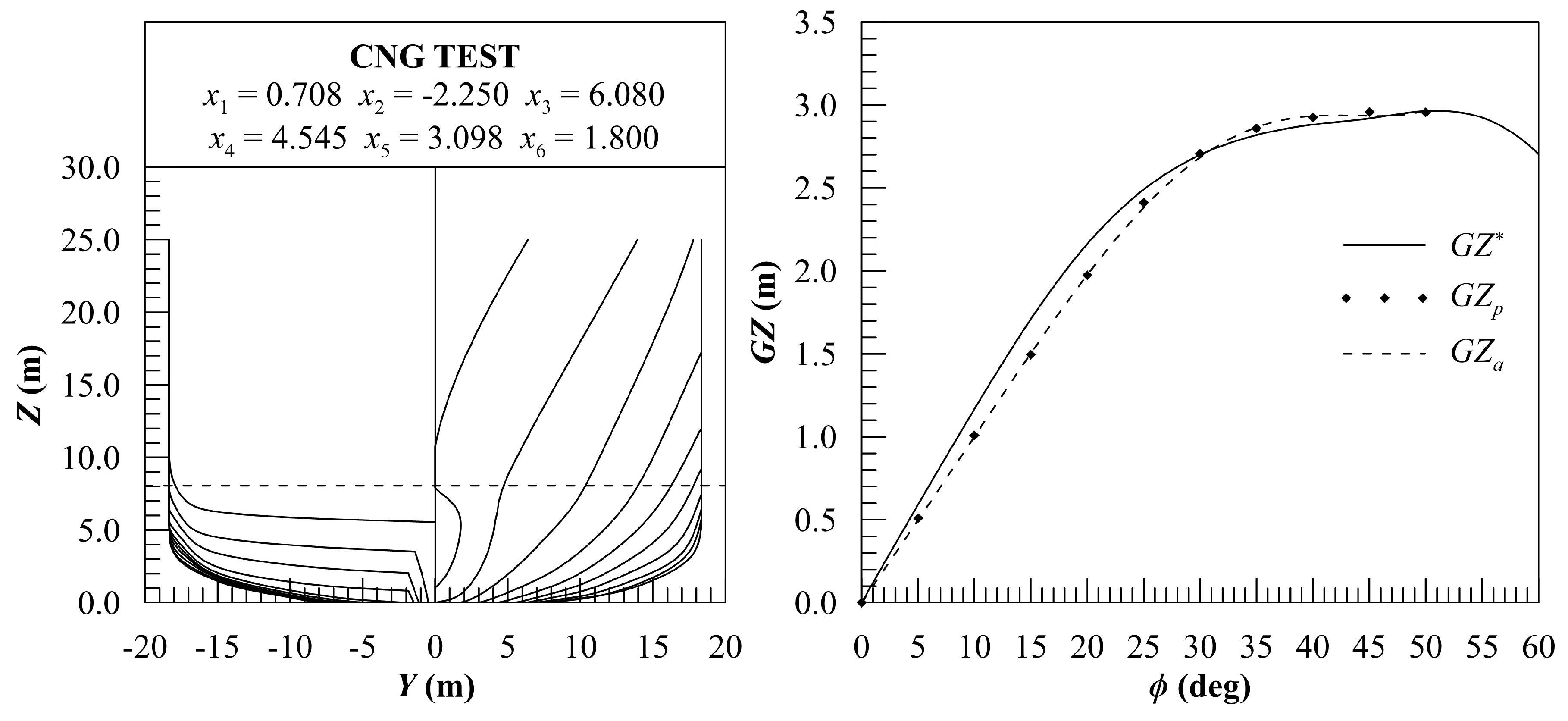
5.1.1. Intact Stability

First, the regression models for intact stability were applied to estimate the $GZ$ curves. In Figure 7, a comparison is presented between the $GZ$ curves from direct calculations, together with the $GZ$ obtained applying the polynomial regressions and the $GZ$ obtained applying the angle-based ones. As can be observed, the two models are quite close to each other, leading almost to the same $GZ$ curve. However, the data coming from direct calculations have a different trend in the first 20 degrees of the curve, even though the determination coefficient $R^2$ for the fitting of the calculated $GZ$ curve is 0.988 for both the polynomial and angle based regression.

The differences in the first part of the $GZ$ curve are related to a different value of the tangent in the origin, which is associated to the initial $GM$ value of a ship. In the presented models for intact stability, the $GM$ is not entering in the set of selected variables, thus the differences may have led to this parameter.

However, it is worth investigating the effect of the changes in the predicted $GZ$ curve on the intact stability criteria described in the previous sections. In

Table 11. Application of stability criteria on the test ship.

Criterion				Values
ID	Description	Limit	Unit	Calculation	Angle-Based	Polynomial
I1	Area $\overline{\varphi }\le 30$ deg	≥ 0.055	m rad	0.829	0.766	0.761
I2	Area $\overline{\varphi }\le min({\varphi }_d,40)$	≥ 0.090	m rad	1.319	1.262	1.257
I3	Area $30\le \overline{\varphi }\le min({\varphi }_d,40)$	≥ 0.030	m rad	0.490	0.497	0.497
I4	$GZ$ at $\overline{\varphi }\ge 30$ deg	≥ 2.0	m	2.966	2.961	2.966
I5	$\overline{\varphi }$ at $maxGZ$	≥ 25.0	deg	51.2	47.2	50.0
W1	${\varphi }_0$	$\le 16$	deg	0.6	0.7	0.7
	Area A	-	m rad	0.426	0.372	0.371
W2	Area B	-	m rad	1.580	1.527	1.521
	Area B ≥ Area A	≥ 1	-	3.711	4.101	4.102

, the values determined to verify the intact stability criteria and the weather criterion are reported. As was reasonable to presume, the regression methods are underestimating the areas under the $GZ$ curve. In fact, the regression curves shown in Figure 7 are lower than the $G{Z}^{*}$ calculated for the test ship, leading to a reduction of about 8% for the area before 30 deg and about 4% for the area before 40 deg. In any case, the criteria are all satisfied, and the deviation of the data coming from regressions is always lower than 20% compared to calculated values.

The geometry and $KG$ of the test CNG ship lead to a condition where there is a lot of reserve of stability, thus the lack in the reproduction of the first part of the curve is not affecting too much the final results, since the ship satisfies the requirements. In the case a condition with less reserve of stability is faced, then the fitting of $GZ$ at low $\varphi$ angles may be an issue that has to be tackled by improving the proposed regressions, adopting a wider range of variables and a wider range of initial ships.

5.1.2. Damage Stability

The geometric floodable lengths were directly calculated for the test ship and then estimated with the proposed model section by section. The values from the direct calculation $GF{L}^{*}$ and the ones from the estimation $GFL$ are shown in Figure 8. The model could reproduce the shape of the curve, resulting in a determination coefficient $R^2$ of 0.920 and a $GFL$ values overestimation of about 7%. The model produced a very good prediction in the midship region while the error increased in the fore and aft ends.

Moreover, it has to be noted that, during concept design, the floodable lengths are assessed aiming at reasonably allocating the main watertight bulkheads. In this sense, the results provided by this preliminary study can be considered promising. In more detail, considering the concept design of a CNG ship, the floodable lengths can be used to define the watertight subdivision in the cargo hold spaces, while, in the other spaces, which are subject to several constraints, can be adopted to check their feasibility in terms of damage stability. Namely, the aft machinery spaces extension is usually defined as a function of the main machinery length and volume (propulsion engines, rudder, steering gears, electric generators, etc.). In the fore compartments, the collision bulkhead shall be fitted according to rules requirements [16] and the second compartment should be dimensioned in order to install the STL system. The longitudinal extension of all these spaces should be kept as small as possible in order to maximise the cargo hold spaces. Hence, no critical problems related to damage stability usually rise in aft and fore areas. Otherwise, the design alternative cannot be simply considered feasible. On the other hand, in the cargo spaces, the number of bulkheads should be minimised since, as already mentioned, the cofferdam spaces entail the loss of an entire row of pressure vessels for each watertight bulkhead.

Applying these ideas on the test ship, the conceptual subdivision was defined. As first, the effective floodable lengths $FL$ were determined dividing the $GFL$ by the permeabilities $\mu$ reported in

Table 12. Standard permeabilities assumed by SOLAS and their application.

Space Type	Permeability	Application
Stores	0.60	Cargo holds
Accommodations	0.95	N.A.
Machinery	0.85	Aft machinery rooms, Engine room, STL space
Void spaces	0.95	Afore collision bulkhead
Liquids	0 or 0.95	Side tanks and double bottom

. According to the authors of [12,13], the main dimensions of aft and fore compartments were defined considering the propulsion system and the STL system. Comparing the length of compartments with the floodable lengths, the subdivision in these regions was found feasible. Then, the remaining watertight boundaries were allocated to obtain the minimal number of constant-length cargo holds. Keeping the same fore and aft spaces, the number of bulkheads in the cargo hold spaces was incremented. The case with no-bulkheads and the one with a single bulkhead were found not feasible, whereas the case of two bulkheads (three cargo holds) was proved to be feasible. The resulting conceptual subdivision layout is provided in Figure 9 that reports both the direct-calculated and estimated floodable lengths, which drove to the same final result. The direct calculation of damage stability finally confirmed the feasibility of the conceptual solution.

6. Conclusions

This paper presents the development and the application of mathematical metamodels for intact and the damage stability of CNG ships during concept design stage. Starting from a set of 45 ships generated by changing systematically six independent variables ($L/B$, $B/T$, $C_B$, $LCB$, $D/T$ and $KG/T$), two models have been developed for the $GZ$ curves determination, applying the RSM technique. Besides, a metamodel is presented to obtain also the $GFL$ starting from the same independent variables. Analysing the determination coefficients of the obtained regressions, all the tested models present a good correlation with the initial population data, being suitable to be applied in the concept design phase of CNG ships. The stepwise technique applied to perform the regressions allows individuating the significant variables per each fitting problem. As a result, it appears that the $L/B$ variations are not affecting the righting arm, while the most influencing variables are $B/T$, $D/T$ and $KG/T$ both for intact and damage stability issues.

The regressions were tested on a ship not included in the initial database, having different hull shape, but with values of the independent variables inside the database boundaries. The regressions could produce $GZ$ and $GFL$ curves and give variations on intact stability criteria values inside 20% with respect to curves obtained by direct calculations. The same was observed for damage $GFL$. Even though the obtained results are satisfactory at a concept design stage, further enhancements can be introduced to the proposed models. In fact, the models are influenced by the initial selection of the independent variables; thus, further study is needed to introduce other variables (and consequently new ships) inside the database. As highlighted by the comparison with the test ship, a possible solution can be the introduction of a variable such as $GM$, to enhance the reproduction of $GZ$ curves at small heeling angles.

With respect to damage stability, the proposed model based on a new definition of the floodable length provided promising results. Although the regressions for damage stability have a lower accuracy compared with the intact stability ones, the model could predict the geometric floodable lengths with an error lower than 15% for the test ship. This accuracy was found sufficient for the concept design phase, allowing to perform a preliminary allocation of all the main watertight boundaries and, in particular, to fit the minimum number of bulkheads in the cargo holds spaces. Applying the proposed process, better estimations of the ship capacity and the weights of the bulkheads and containment system are possible at the concept design phase. However, future work is required to enhance the accuracy of the predictions, especially in the aftermost and foremost zones, as highlighted by the test case. Finally, the application of different techniques devoted to a more rational bulkhead arrangement could be adopted to maximise the number of the pressure vessels, going beyond the assumption of constant-length cargo holds.

It is worth noticing that the developed stability metamodels require an estimation of the ship weight and the centre of mass. In the presented study, only the stability metamodels were analysed, thus they are decoupled with ship weight estimation. Inside an MCDM process, the obtained models are structured in such a way to use data coming from a dedicated simplified ship weight estimation metamodel, which is why the variable $KG/T$ has been introduced. Weight estimation is planned to be analysed more in detail in further research, which may also lead to a coupling of the two issues.

References

- Trincas, G. Survey of design methods and illustration of multiattributes decision making system for concept ship design. In Proceedings of the MARIND 2001, Varna, Bulgaria, 12–14 October 2001. [Google Scholar]
- Gaggero, T.; Vernengo, G.; Parodi, M.; Rizzuto, E. Logistics-based fleet design for complex transport scenarios. Ships Offshore Struct. 2018, 13, 734–749. [Google Scholar] [CrossRef]
- Valsgård, S.; Reepmeyer, O.; Lothe, P.; Strøm, N.; Mørk, K. The development of a compressed natural gas carrier. In Proceedings of the 9th International Symposium on Practical Design of Ships and Other Floating Structures (PRADS), Lübeck-Travemünde, Germany, 12–17 September 2004. [Google Scholar]
- Lothe, P. The Knutsen OAS shipping pressurized natural gas carrier (PNG). In Proceedings of the Fifteenth International Offshore and Polar Engineering Conference (ISOPE), Seoul, Korea, 19–24 June 2005. [Google Scholar]
- Nikolau, M.; Wang, X.; Economides, M. Optimisation of compressed natural gas marine transportation with composite-material containers. In Proceedings of the SPE Asia Pacific Oil and Gas Conference and Exibition, Jakarta, Indonesia, 22–24 October 2013. [Google Scholar]
- Arias, C.; Herrador, J.; del Castillo, F. Intact and damage stability assessment for the preliminary design of a pasenger vessel. In Proceedings of the 8th International Conference on the Stability of Ships and Ocean Vehicles (STAB), Madrid, Spain, 15–19 September 2003. [Google Scholar]
- Economides, M.; Wood, D. The state of natural gas. J. Nat. Gas Sci. Eng. 2009, 1, 1–13. [Google Scholar] [CrossRef]
- Bortnowska, M. Development of new technologies for shipping natural gas by sea. Pol. Marit. Res. 2009, 16, 70–78. [Google Scholar] [CrossRef] [Green Version]
- Nikolau, M. Optimizing the logistics of compressed natural gas transportation by marine vessels. J. Nat. Gas Sci. Eng. 2010, 2, 1–20. [Google Scholar] [CrossRef]
- Wagner, J.; van Wagensveld, S. Marine transportation of compressed natural gas a viable alternative to pipeline or LNG. In Proceedings of the SPE Asia Pacific Oil and Gas Conference and Exibition, Melbourne, Australia, 8–10 October 2002. [Google Scholar]
- Trincas, G. Comparison of Marine Technologies for Mediterranean Offshore Gas Export. In Proceedings of the 19th international conference on Ship & Maritime Research (NAV 2018), Trieste, Italy, 20–22 June 2018. [Google Scholar] [CrossRef]
- Mauro, F.; Braidotti, L.; Trincas, G. Determination of an optimal fleet for a CNG transportation scenario in the Mediterranean Sea. Brodogradnja 2019, 70, 1–23. [Google Scholar] [CrossRef]
- Trincas, G.; Mauro, F.; Braidotti, L.; Bucci, V. Handling the path from concept to preliminary ship design. In Marine Design XIII; CRC Press: Boca Raton, FL, USA, 2018; Volume 1, pp. 181–192. [Google Scholar]
- Mauro, F.; Braidotti, L.; Trincas, G. Effect of Different Propulsion Systems on CNG Ships Fleet Composition and Economic Effectiveness. In Proceedings of the 19th international conference on Ship & Maritime Research (NAV 2018), Trieste, Italy, 20–22 June 2018. [Google Scholar] [CrossRef]
- IMO. Intact Stability Code; International Maritime Organization: London, UK, 2008. [Google Scholar]
- IMO. International Gas Code; International Maritime Organization: London, UK, 2016. [Google Scholar]
- ABS. Guide for Vessels Inteded to Carry Compressed Natural Gasses in Bulk; ABS: Huston, TX, USA, 2017. [Google Scholar]
- DNV-GL. Rules for Classification of Ships. Pt.5 Ch.15 Compressed Natural Gas Carrier; DNV-GL: Høvik, Norway, 2016. [Google Scholar]
- Chang, H. A data mining approach to dynamic multiple responses in Taguchi experimental dsign. Expert Syst. Appl. 2008, 35, 1095–1103. [Google Scholar] [CrossRef]
- Mauro, F.; Dell’Acqua, A. Vertical Motions Assessment of an Offshore Supply Vessel in Concept Design Stage. In Proceedings of the 19th international conference on Ship & Maritime Research (NAV 2018), Trieste, Italy, 20–22 June 2018. [Google Scholar] [CrossRef]
- Myers, R.; Montgomery, D.; Anderson-Cook, C. Response Surface Methodology—Process and Product Optimization Using Designed Experiments, 3rd ed.; J. Wiley & Sons: Hoboken, NJ, USA, 2008. [Google Scholar]
- Beaver, R.; Montgomery, D. Design and Analysis of Experiments. Biometrics 1977, 33, 273–283. [Google Scholar] [CrossRef] [Green Version]
- Montgomery, D. Design & Analysis of Experiments, 7th ed.; J. Wiley & Sons: Hoboken, NJ, USA, 2009. [Google Scholar]
- Braidotti, L.; Mauro, F. A New Calculation Technique for Onboard Progressive Flooding Simulation. Ship Technol. Res. 2019, 66, 150–162. [Google Scholar] [CrossRef]
- Lai, T.; Robbins, H.; Wei, C. Strong consistency of least squares estimates in multiple regression. Proc. Natl. Acad. Sci. USA 1978, 75, 3034–3036. [Google Scholar] [CrossRef] [PubMed] [Green Version]
- Harrell, F. Regression Modelling Strategies: With Application to Linear Models, Logistic Regression, and Survival Analysis; Springer: New York, NY, USA, 2001. [Google Scholar]
- Taylan, M. The effect of nonlinear damping and restoring in ship rolling. Ocean. Eng. 2000, 27, 921–932. [Google Scholar] [CrossRef]
- Mauro, F.; Nabergoj, R. Determination of non-linear roll damping coefficients from model dacaytest. In Proceedings of the Engineering Mechanics (EM 2017), Svratka, Czech Republic, 15–18 May 2017. [Google Scholar]
- Oliva-Remola, A.; Bulian, G.; Perez-Rojas, L. Estimation of damping through internally excited roll tests. Ocean. Eng. 2018, 160, 490–506. [Google Scholar] [CrossRef]
Figure 1.
Sketch of the weather criterion requirements according to ISC 2008.
Figure 2.
Example of a set of CNG hull-forms together with the associated and curves.
Figure 3.
Calculated vs. estimated non-dimensional values (left) and associated per each vessel inside the database (right) according to polynomial regression method.
Figure 4.
Calculated vs. estimated non-dimensional values (left) and associated per each vessel inside the database (right) according to angle-based regression method.
Figure 5.
Calculated vs. estimated non-dimensional values (left) and associated per each ship inside the database (right) imposing equal to 0 for unstable ships.
Figure 6.
Calculated vs. estimated non-dimensional values (left) and associated per each ship inside the database (right).
Figure 7.
The body plan for the test ship and the related curves according to direct calculation and the two proposed regression models.
Figure 8.
curves for the test ship according to direct calculation and the proposed regression model.
Figure 9.