Abstract
The seabed is usually non-homogeneous in the real marine environment, and its response to the dynamic wave loading is of great concern to coastal engineers. Previous studies on the simulation of a non-homogeneous seabed response have mostly adopted a vertically layered seabed, in which homogeneous soil properties are assumed in the governing equations for one specified layer. This neglects the distribution gradient terms of soil property, thus leading to an inaccurate evaluation of the dynamic response of a non-homogeneous seabed. In this study, a numerical model for a wave-induced 3D non-homogeneous seabed response is developed, and the effects of the soil property distribution gradient on the wave-induced response of a non-homogeneous seabed are numerically investigated. The numerical model is validated, and the results of the present simulation agree well with those of previous studies. The validated model is applied to simulate an ideal two-dimensional (2D) vertical non-homogeneous seabed. The model is further applied to model the practical wave-induced dynamic response of a three-dimensional (3D) non-homogeneous seabed around a mono-pile. The difference in pore pressure and soil effective stresses due to the soil distribution gradient is investigated. The effects of the soil distribution gradient on liquefaction are also examined. Results of this numerical study indicate that (1) pore pressure decreases while soil effective stresses increase (the maximum difference of the effective stresses can reach 68.9) with a non-homogeneous seabed if the distribution gradient terms of soil properties are neglected; (2) the effect of the soil property distribution gradient terms on the pore pressure becomes more significant at the upper seabed, while this effect on the soil effective stresses is enhanced at the lower seabed; (3) the effect of the soil distribution gradient on the seabed response is greatly affected by the wave reflection and diffraction around the pile foundation; and (4) the soil distribution gradient terms can be neglected in the evaluation of seabed liquefaction depth in engineering practice.
1. Introduction
A marine structure usually suffers from complex coastal environmental loadings, such as winds, waves, currents, etc. [1,2,3], and studying its stability has attracted lots of attention from coastal engineers. The wave-induced seabed response is of significant importance to the construction of marine structures because it can lead to seabed instability around a structure’s foundation [4]. Excess pore pressures can occur as a result of the dynamic wave pressure at the seabed surface. When excess pore pressure exceeds the overburden pressure, the effective stresses of the soil skeleton vanish, and the soil behaves like a liquid. This phenomenon is referred to as liquefaction, and it can lead to the collapse of the marine structure [5,6]. Smith and Gordon [7] reported that the failure of marine structures was predominantly caused by wave-induced seabed instability rather than structural deficiencies. Therefore, it is important to investigate the seabed dynamic response to wave loading in order to evaluate seabed instability.
On the basis of Biot’s consolidation theory, Yamamoto et al. [8] were among the first to study the wave-induced seabed response. In their study, analytical solutions for the seabed dynamic response were given for pore pressures, soil effective stresses, and soil displacements. Using a similar approach, Madsen [9] analytically investigated the seabed response with an isotropic soil property. Jeng and Hsu [10] extended the above analytical solutions to the seabed with finite depth and studied the seabed dynamic response using the 3D short-crested wave loading. These investigations adopted Q-S (Quasi-Static) equations, which neglect the inertial terms of pore pressure and the soil skeleton [11]. To consider the inertial term of soil, Jeng and Rahman [12] used a PD model (partial dynamic) to analytically investigate the wave-induced seabed response. They found a difference in pore pressure between the Q-S and P-D models for the same case. Ülker and Rahman [13] used a similar approach to investigate the seabed response and clarified the application range of the QS, PD, and FD (fully dynamic) models. Liao et al. [14] and Tong et al. [15] considered the effect of currents on the wave-induced seabed response, and Chen et al. [16] studied the nonlinear wave-induced response of an anisotropic seabed. Similar studies have been conducted to investigate the seabed response around marine structures, such as pipelines [17], composite breakwaters [18,19,20,21,22], and mono-piles [23,24]. All these studies have assumed a homogeneous seabed that adopts constant soil parameters in space.
Because consolidation occurs over a long time, the seabed, in reality, is usually non-homogeneous in the vertical direction [25]. Yamamoto [26] analytically investigated the wave-induced response of a vertically layered seabed at the Mississippi Delta. He found that a seabed with a vertical depth of 1/5 wavelength was the most unstable that and landslides could occur during a storm. Rahman et al. [27] presented a semi-analytical solution for the multi-layered seabed response and applied it with the 3D short-crested wave loading in front of a vertical breakwater. On the basis of the TRM method, Zhou et al. [28] proposed an analytical solution for a vertically layered seabed under the nonlinear wave loading. Considering the inertial terms of pore fluid and soil skeleton, Ülker [29] used a semi-analytical method to investigate the multi-layered seabed response. Effects of non-homogeneous soil properties on the seabed response against the inertial terms were examined in the study. Most of the above studies have adopted a so-called “layered” seabed in which the homogeneous soil properties were assumed in one specified layer. This neglects the distribution gradient terms of non-homogeneous soil properties in the governing equations and may lead to an inaccurate evaluation of the dynamic response in a non-homogeneous seabed. Jeng and Lin [30] developed a 2D finite element model for the wave-induced seabed response and assumed a continuous variation in non-homogeneous soil properties. The distribution gradient terms of soil properties were considered in the governing equations (QS model) of their study. Similar research can be seen in Zhang et al. [31] for a randomly heterogeneous porous seabed. More recently, Chen et al. [32] applied a 3D model for a non-homogeneous seabed, but they only considered the non-homogeneous properties and retained the gradient term in the vertical () direction. Using the FD model equations, Zhang et al. [33] developed a 3D numerical model for the non-homogeneous seabed response. Their study retained all the gradient terms of the soil parameters, but the gradient terms in the governing equations were not fully separated out. They only compared the seabed dynamic response between a homogeneous seabed and non-homogeneous seabed, and the soil property distribution gradient terms in the non-homogeneous seabed, which play an important role, were not quantitatively examined. To the authors’ knowledge, the quantitative effects of the soil distribution gradient on the response of a non-homogeneous seabed have not yet been investigated.
This study focuses on the non-homogeneous seabed, in which the effects of the soil distribution gradient are emphasized. Compared with the authors’ previous work in Zhang et al. [33], the contributions of this study are summarized: (1) the distribution gradient terms of non-homogeneous soil properties are separated out on the basis of the original governing equations of the soil dynamic response; (2) the effects of the distribution gradient on the soil dynamic response (pore water pressures, soil effective stresses) and liquefaction are examined. In a word, the previous studies in Jeng and Lin [30] and Zhang et al. [33] compared the soil responses between the homogeneous seabed and non-homogeneous seabed, while this study focuses on the non-homogeneous seabed and compares cases with and without the property distribution gradient terms. The outline of this paper is as follows. The governing equations (FD model) for the wave-induced seabed response are newly derived in Section 2, and the distribution gradient terms of soil properties are clearly highlighted. Model validations are then presented by comparing the present numerical results with available experimental data and field measurements. The validated model is then applied to evaluate the differences in pore pressure and soil effective stresses due to soil distribution gradient terms. Results are presented in Section 3 and Section 4, in which the effects of the property gradient on the seabed response are examined by simulating an ideal 2D non-homogeneous seabed (Section 3) and a more realistic 3D non-homogeneous seabed around a mono-pile foundation (Section 4). Liquefaction analysis is presented in Section 5. Detailed discussions are presented in Section 6 and highlight the contributions of this study. Finally, the main conclusions from this study are presented in Section 7.
2. Numerical Model
This study adopts the FD model for the wave-induced seabed response. The governing equations are presented with the soil distribution gradient terms highlighted. Boundary conditions are provided to solve the nonlinear partial equations of the numerical model, which is validated using flume tests [34] and field measurements [26].
2.1. Seabed Model
On the basis of Biot’s consolidation theory, the FD model for the seabed response that considers the inertial terms of pore pressure and soil skeleton is
where is the total stresses (i and j denote the directions of x, y, z in the Cartesian system), that is or or for , and or or for . is the average density of the porous medium, p denotes pore pressure, is water density, is gravitational acceleration in the i-direction, is the displacement of the soil matrix in the i-direction, is the average relative displacement of the fluid to the solid skeleton in the i-direction, is the permeability of the porous medium in the i-direction, and n is the porosity of soil. It should be noted that the above FD model will be reduced to the PD model by ignoring the accelerations due to pore water, while the PD model will be reduced to the QS model by further ignoring the acceleration due to the soil skeleton. The equivalent compressibility of pore water and entrapped air is defined as [8]
where d is the water depth, is the saturation degree, and is the bulk modulus of pure water and is taken as N/m. A poroelastic constitutive model of soil is adopted to govern the deformation of the soil skeleton. The total stresses can be written as
where is the Kronecker delta denotation which equals 0 for or 1 for i and j, respectively. denotes the soil effective stresses and shear stresses. In this study, cross-anisotropic soil behavior is adopted:
where , , and are the Poisson ratios in different directions. Noted here that, h denote the horizontal plane including x and y directions, v denote the vertical direction z, the subscript in means a contraction in direction x or y when an extension is applied in direction z. Similar explanations are with and . and are Young’s modulus in the horizontal and vertical directions, respectively; and are shear modulus in the horizontal and vertical directions, respectively; is a non-dimensional parameter; and is the anisotropic constant. Note that for an isotropic seabed, = , , and .
A poroelastic constitutive model of soil is adopted to govern the deformation of the soil skeleton. Thus, the effective stress–strain relation can be written as [35]:
where
In the present model, eight soil parameters are allowed to vary non-homogeneously, which is the function of spatial locations. These parameters are the porous media density , water density , permeability , the porosity of the solid phase , the bulk modulus of pore water , vertical Young’s modulus , vertical Poisson’s ratios , and horizontal Poisson’s ratios .
The velocity of pore water can be obtained from Equation (2):
From the above definitions, the governing equations can be derived. Substituting Equations (9)–(14) into Equations (1)–(3) and replacing the velocity of the pore pressure in Equation (3) with Equation (20) yield the governing equations for the dynamic response of a non-homogeneous seabed in the scalar form:
Note that, this study obtained (velocity of pore water) (20) from (2) (seepage equilibrium equation) and combine it with (3) (Mass continuous equation), thus all the gradient terms are separated out (see the underlined for k and E) in the governing Equations (21)–(27). Equations (20) and (27) are newly proposed in this study. Comparing to the previous studies, this study provide a approach to separate out all the gradient terms in the 3D dynamic response equations of the elastic porous seabed medium.
2.2. Boundary Conditions
Several boundary conditions need to be specified to solve the partial differential governing equations. The lateral sides and the bottom of the seabed are considered to be rigid and non-permeable; thus, the displacement of soil and the pore pressure gradient at those points equal zero:
At the seabed/water interface, the pore pressure is equal to the dynamic wave pressure at the seabed surface while the soil vertical normal effective stresses and shear stresses vanish. On the basis of linear wave theory, the dynamic wave pressure for the propagation wave is [4]:
where H is the wave height, is the wavenumber, is the wave frequency, and is the wave pressure at the seabed surface and is provided by the nonlinear wave model FUNWAVE 2.0. The FUNWAVE 2.0 Code was first developed by Kirby [36] on the basis of the nonlinear Boussinesq equations [37], and it is widely used to simulate the nonlinear wave–structure interactions in coastal areas. The phenomenon of wave reflection and diffraction around a mono-pile foundation can be well represented with the FUNWAVE 2.0 model [23]. Readers interested in the FUNWAVE 2.0 Code can refer to Kirby [36].
2.3. Model Validation
Model validation must be conducted before we can confidently apply the numerical model. Figure 1 is the comparison of the measured [34] and simulated (this study) vertical distributions of pore pressure. The analytical solution of Jeng [38] is also included for comparison. Pore pressure is seen to be relatively large at the seabed surface, and it sharply decreases at the deep soil. Figure 1 shows that vertical pore pressure depends significantly on the wave and seabed conditions. Results indicate that the large pore pressure within the seabed usually corresponds to a relatively large wave period (T) and soil saturation degree () for otherwise identical conditions. Good agreement is found between the simulation and the experimental data [34], as well as the analytical solution [38], indicating that the present model has high accuracy in simulating the seabed dynamic response.
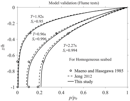
Figure 1.
Comparison of the measured [34] and simulated (this study) vertical distributions of pore pressure.
The seabed in the real coastal environment is usually non-homogeneous, which will significantly change the pore pressure in the vertical direction. Bennett and Faris [25] performed field measurements at the Mississippi Delta to measure the pore pressure distributions and attenuations in the vertical direction of the seabed. Yamamoto [26] assumed a constant saturation degree of soil and investigated the pore pressure distributions using analytical solutions. Figure 2 shows the comparison of the measured [25] and simulated pore pressures (this study), as well as the analytical solution from Yamamoto [26]. It is seen in Figure 2 that there exist large discrepancies between the measured [25] and theoretical results [26]; in the latter study, a constant saturation degree of = 0.9 or = 1.0 was used. In this study, a non-homogeneous saturation degree of soil is adopted with a linear variation in depth (), which obtains good agreement with the measured data by Bennett and Faris [25]. This validation example indicates that the non-homogeneity of soil is important and has to be considered in the simulation.
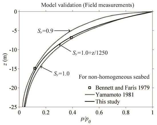
Figure 2.
Comparison of the measured [25] and simulated pore pressures (this study) in the vertical seabed at Mississippi Delta.
3. 2D Vertical Non-Homogeneous Seabed
An ideal 2D case for the wave-induced dynamic response of a vertical non-homogeneous seabed is studied (Figure 3) by considering the continuous variation in non-homogeneous soil properties (permeability and Young’s modulus). Previous studies have indicated that the porosity of the soil skeleton generally decreases with the increase in seabed depth, therefore leading to the decrease in soil permeability and the increase in the soil Young’s modulus [30,39]. Therefore, the model setup in this study adopts this distribution trend for soil permeability and Young’s modulus. Nine numerical examples, which are indicated by the symbol ( and ), are run for the 2D case. The subscript denotes the three categories of the depth function () for non-homogeneous permeability ( denotes soil permeability at the seabed surface). Type 1 () is for and represents uniform permeability of the seabed. Type 2 () is for , denoting linear variation in permeability. Type 3 () is for , denoting an exponential relation in permeability with depth. Similarly, the subscript denotes the three categories of the depth function () for seabed Young’s modulus and are defined as (type 1, ), (type 2, ), and (type 3, ). Details of the wave and seabed parameters used in the simulations are listed in Table 1. The sketch of model setup for the non-homogeneous seabed response is illustrated in Figure 3a. Details of non-homogeneous permeability and Young’s modulus () distributions can be seen in Figure 3b,c. When and are equal to 1 (type 1 for and ), it reflects a homogeneous seabed with constant properties. For the non-homogeneous and , the distribution gradient (decreasing) of () (Figure 3b) with type 3 is larger than that with type 2 at the upper seabed (see the tangent slope), while it is smaller at the lower seabed. In contrast, the distribution gradient (increasing) of (Figure 3c) with type 3 is smaller at the upper seabed and larger at the lower seabed (Figure 3c). Note that this difference in the distribution gradient between and has a significant influence on the wave-induced non-homogeneous seabed response (see below).
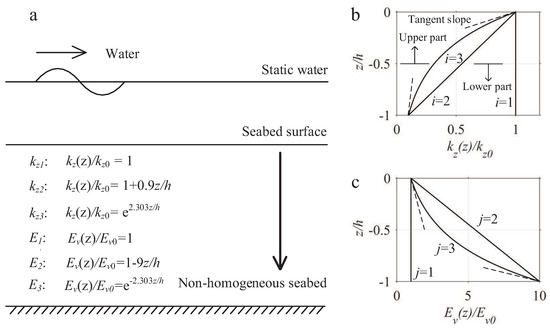
Figure 3.
Model setup for the non-homogeneous seabed response: (a) Sketch map, (b) distribution of non-homogeneous permeability (k), (c) distribution of non-homogeneous Young’s modulus (E).

Table 1.
Wave and seabed parameters used in this study (2D case).
Figure 4 illustrates the comparison of pore pressure with (solid line) and without (red dashed line) the gradient terms in the governing equations for a non-homogeneous seabed in which is the maximum pore pressure within one wave period, and is the maximum pore pressure () at the seabed surface. It is seen from Figure 4 that the pore pressure at the seabed surface () equals the dynamic wave pressure and decreases with the increase in seabed depth. No discrepancies in pore pressure between the case with and without the gradient terms are found with case (Figure 4a). This is because the distribution gradient of and equals zero with a homogeneous seabed. The first row of the nine subfigures (Figure 4a–c for cases , , and , respectively) indicates the change in the distribution gradient with a constant . It clearly shows that the pore pressure increases if the gradient term of is neglected. In addition, the discrepancies in pore pressure are only found at the lower part of the seabed, indicating that the effect of Young’s modulus gradient term () is limited to the region near the seabed bottom (). Meanwhile, the discrepancies in pore pressure (, caused by the gradient term) increase in the order , , and , which is probably because the gradient of Young’s modulus increases in that order at the lower seabed (Figure 3). The first column (Figure 4a,d,g for cases , , and , respectively) shows the change in the distribution gradient with a constant . In contrast to (Figure 4a–c), the pore pressure decreases if the gradient term of is neglected. The pore pressure discrepancy caused by the permeability gradient () mainly exists at the upper part of the seabed (around ), which indicates that the permeability gradient has a more significant influence at that part. It also illustrates that the discrepancy in pore pressure increases in the order , , and , which is mainly because the gradient of permeability increases in that order at the upper seabed. The other subfigures (Figure 4e,f,h,i for cases , , , and , respectively) reflect a seabed in which and are both non-homogeneous. An interesting phenomenon is found: the pore pressure decreases at the upper part while increasing at the lower part of the seabed. This is probably the result of the combined influence of the distribution gradient in and .
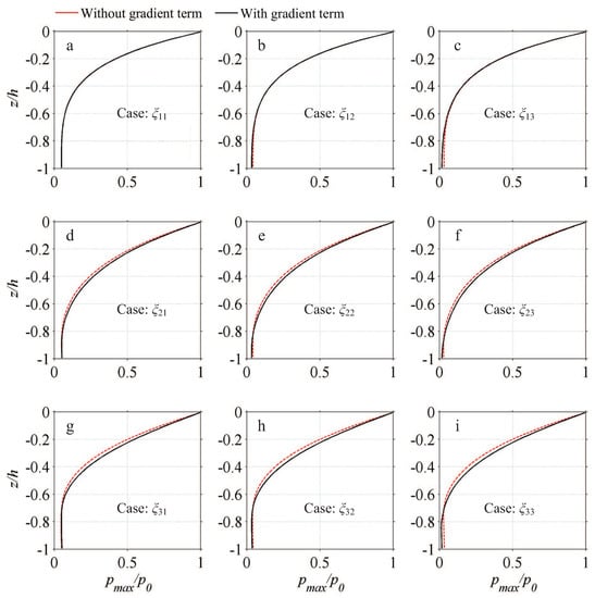
Figure 4.
Comparison of pore pressure with (solid line) and without (red dashed line) the gradient terms of the governing equations in a non-homogeneous seabed: (a) Case , (b) Case , (c) Case , (d) Case , (e) Case , (f) Case , (g) Case , (h) Case , (i) Case .
The maximum pore pressure discrepancy () due to the distribution gradient of non-homogeneous properties is quantitatively shown in Figure 5, in which ), while ) and respectively indicate the pore pressure without and with the gradient term of soil properties. Therefore, can be seen as the effect of the property gradient on the non-homogeneous seabed response. Figure 5a shows for cases of , , and , and it represents the quantitative effect of the Young’s modulus gradient term (). As indicates the case with a homogeneous seabed (), with is equal to zero accordingly. It shows for and for , indicating that the distribution gradient effect of is more significant if the exponential variation of distribution is adopted (). By comparison, Figure 5b shows for cases of , , and , and it describes the quantitative effect of the permeability gradient (). Similar to that in Figure 5a, the maximum is found with , indicating that the largest effect of the gradient occurs for exponential variation (). It is also found that the maximum induced by the gradient is larger than the maximum induced by the gradient. This indicates that the pore pressure (p) is more sensitive to the permeability () distribution gradient.
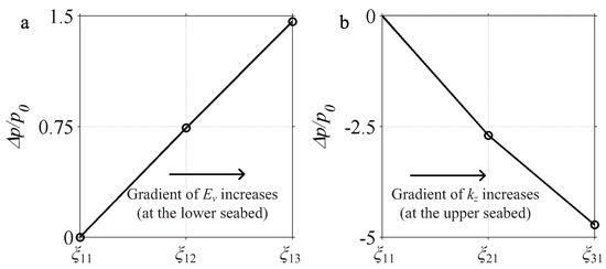
Figure 5.
Quantitative study on the maximum pore pressure discrepancies () due to (a) the Young’s modulus gradient and (b) the permeability gradient.
Figure 6 shows the comparison of soil effective stresses () with (solid line) and without (red dashed line) the gradient terms of the governing equations for a non-homogeneous seabed. It is shown that the soil effective stresses () vanish at the seabed surface because there is no compaction of soil particles there. It is seen in Figure 6a–c (the change in the gradient with constant ) that the soil effective stresses () increase if the gradient of Young’s modulus is neglected. The largest discrepancy in the soil effective stresses () is found at the seabed bottom. This phenomenon is similar to that of the pore pressure () distribution (Figure 4), except that the discrepancy in the soil effective stresses () is much larger than that with pore pressure. Figure 6a,d,g (the change in the gradient with constant ) show that the soil effective stresses () increase if the permeability gradient is neglected. The discrepancy in the soil effective stresses () caused by the permeability gradient is insignificant and mainly appears at the upper seabed. Finally, Figure 6e,f,h,i (non-homogeneous and ) demonstrate that the soil effective stresses () increase if the gradients of properties (both and ) are neglected. It is also found that the distribution pattern of in the case , is similar to that in the case , while in , is similar to that in . This means that the Young’s modulus distribution gradient () dominates the distribution pattern of .
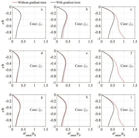
Figure 6.
Comparison of soil effective stresses () with (solid line) and without (red dashed line) the gradient terms of the governing equations ( is the maximum pore pressure at the seabed surface): (a) Case , (b) Case , (c) Case , (d) Case , (e) Case , (f) Case , (g) Case , (h) Case , (i) Case .
Figure 7 is the quantitative analysis of the maximum soil effective stress discrepancy () caused by (a) the Young’s modulus gradient and (b) the permeability gradient. It is found that the discrepancy in the soil effective stresses () with is equal to zero, which is also the case for the homogeneous seabed. Figure 7a illustrates the for , and , and it shows the gradient effect of Young’s modulus on the soil effective stresses. Figure 7a reveals that for the case and for the case . These results indicate that the largest effect of the Young’s modulus gradient on the soil effective stresses occurs when the variation in (case ) is exponential. In addition, Figure 7a also shows for , , and , and it shows the effect of the permeability gradient () on the soil effective stresses. It is seen that for the case is larger than for the case , indicating that the permeability gradient has a greater effect for the exponential variation of (). It is also found that the maximum caused by the distribution gradient is much larger than the maximum caused by the distribution gradient. This indicates that the distribution of soil effective stresses () is more sensitive to the Young’s modulus () distribution gradient.
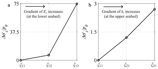
Figure 7.
Quantitative analysis on the maximum soil effective stress discrepancies () due to (a) the Young’s modulus gradient and (b) the permeability gradient.
The above quantitative analysis (Figure 5 and Figure 7) involves the cases of only non-homogeneous Young’s modulus () with constant permeability (k) (case , ) or the cases of only non-homogeneous permeability (k) with constant Young’s modulus () (case , ). Figure 8 illustrates the quantitative analysis of and for non-homogeneous seabed with both non-homogeneous permeability and Young’s modulus (, , , and ). It clearly shows that all the values of are positive, while all values are negative, which indicates that the soil effective stresses (pore pressure p) increase (decrease) if the property gradient is neglected. In addition, the discrepancies (, , , and ) are generally greater than (, , , and ). This confirms, by comparison with the pore pressure (p), that the soil effective stresses () are more easily affected by the property distribution gradient of a non-homogeneous seabed.
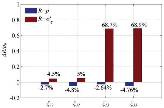
Figure 8.
Quantitative analysis of the discrepancies in pore pressure and soil effective stresses for a seabed with both non-homogeneous permeability and Young’s modulus (cases , , , and ).
4. 3D Non-Homogeneous Seabed around a Mono-Pile
A mono-pile is commonly used as a support for marine structures, such as offshore wind turbines, platforms, and sea bridges. Most previous studies have indicated that the long-term rocking of a mono-pile will cause size sorting of the soil particles around the pile. This may be because smaller-sized particles have high mobility and can move into the deep seabed. As a result, a 3D non-homogeneous seabed is generated accordingly. This inverse grading of soil particles is referred to as the “Brazil nut effect” [40,41]. Cuéllar et al. [41] experimentally investigated particle size sorting around a long-term rocking mono-pile. They found that two seabed zones, named the convected zone (within the inverted cone in Figure 9a) and static zone (outside the inverted cone in Figure 9a), emerged around the mono-pile after approximately 5 million cycles of rocking (horizontal) of the pile (Figure 9). Particle size sorting is only found within the convected zone, in which the relatively coarser soil is at the upper part, while the relative finer soil is at the lower part of the seabed. It is noted that the seabed in the static zone is not affected by the rocking of the pile.
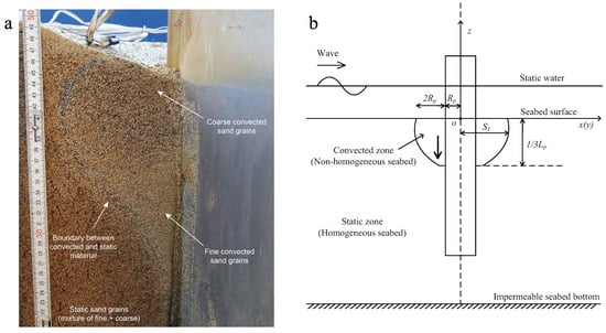
Figure 9.
(a) A 3D non-homogeneous seabed around the pile in (a) the experimental study of Cuéllar et al. (adopted from reference [41], have got the permission from springer) and (b) the numerical model setup of this study.
On the basis of the study by Cuéllar et al. [41], this study assumes a homogeneous seabed within the static zone and a non-homogeneous seabed within the convected zone (Figure 9b). The radius of the convected zone at the seabed surface is three times that of the pile radius (), and the depth is times the pile insertion length (). In addition, with increasing depth, the soil permeability decreases while Young’s modulus increases. The linear relationship of soil property variation is adopted for the first approximation. The interface between the convected zone and the static zone is described as
where is the distance from the interface to the middle line of the pile (Figure 9b), which is depth-dependent in this study. Note that Zhang et al. [33] only adopted a linear wave theory in which wave transformations around the mono-pile were not considered. In this study, the non-homogeneous seabed response is investigated while considering wave reflection and diffraction. Furthermore, the discrepancies in pore pressure (p) and soil effective stresses () caused by the property distribution gradient in a non-homogeneous seabed are examined. The pile radius () is set at 2.5 m and the pile insertion depth () is 8 m. Other parameters for the wave and seabed are listed in Table 2, and the sketch of the model setup is illustrated in Figure 9b.
Table 2.
Wave and seabed parameters used in this study (3D case).
Figure 10 illustrates the distribution of maximum pore pressures for (a) a non-homogeneous seabed (), (b) a homogeneous seabed (), and (c) their difference () around a mono-pile foundation. It is found that the magnitude of pore pressures is larger at the head of pile than at the rear. This is because the wave reflection in front of the pile will lead to greater wave loading there. By comparing Figure 10a with Figure 10b, it can also be found that the pore pressure a with non-homogeneous seabed is much larger than that with a homogeneous seabed. The largest difference caused by non-homogeneous soil properties is in front of the pile (Figure 10c). This is because the soil permeability is larger in the convected zone of the non-homogeneous seabed, thus making it easier for the pore pressure to penetrate the seabed.
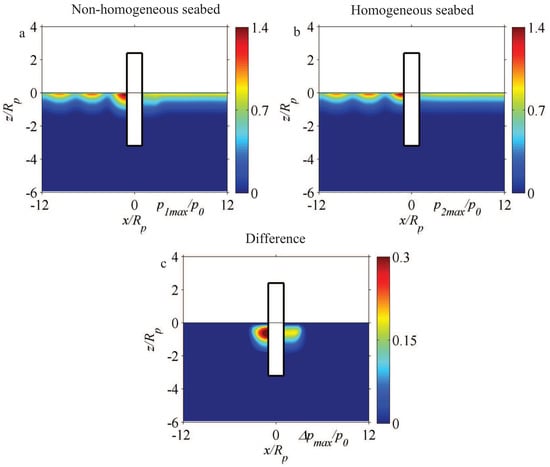
Figure 10.
The distribution of maximum pore pressures with (a) a non-homogeneous () (b) a homogeneous seabed (), and (c) their difference () around a mono-pile foundation.
Figure 11 illustrates the distribution of maximum soil effective stresses for (a) a non-homogeneous seabed (), (b) a homogeneous seabed (), and (c) their difference () around a mono-pile foundation. Similar to the pore pressure (Figure 10), the soil effective stresses are also larger in front of the pile because of wave reflection and diffraction (Figure 11a,b). However, contrary to the larger pore pressure found with a non-homogeneous seabed (Figure 10), the soil effective stresses are smaller if a non-homogeneous seabed is considered (Figure 11c). This is because the total force of the soil skeleton will be balanced by the combination of pore pressure and soil effective stresses. Therefore, the increase in pore pressure in a non-homogeneous seabed will naturally lead to a decrease in the soil effective stresses.
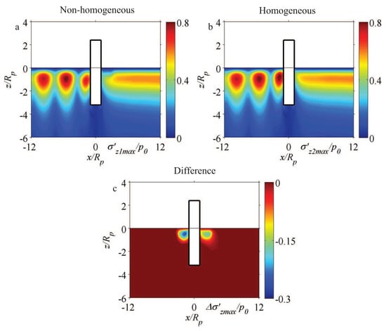
Figure 11.
The distribution of maximum soil effective stresses with (a) a non-homogeneous seabed (), (b) a homogeneous seabed (), and (c) their difference () around a mono-pile foundation.
Figure 10 and Figure 11 above compares the seabed response between a non-homogeneous and homogeneous seabed. Next, Figure 12 illustrates the discrepancy in (a) the pore pressure and (b) the soil effective stresses caused by the soil property gradient term in a non-homogeneous seabed around a mono-pile (in the x-direction, , m). The convected zone and static zone are specified around the mono-pile (Figure 12). It is found that the pore pressure (p) and the soil effective stresses () increase (decrease) in front (at the rear) of the mono-pile because of the wave reflection and diffraction. In addition, the gradient term of non-homogeneous soil properties has a great influence on the distribution of p and . Specifically, the pore pressure decreases (Figure 12a) while the soil effective stresses increase (Figure 12b) if the gradient term is neglected. This is consistent with the main findings of the gradient effects on p (Figure 4) and (Figure 6) for the 2D case in this study. In addition, the discrepancy in the pore pressure () and the soil effective stresses () is found to be larger in front of the pile (, ) in comparison with that found at the rear (, ), which is probably because the wave pressure is larger there (see the relevant discussions in Figure 10 and Figure 11). This indicates that the effect of the soil property distribution gradient on the seabed response is larger in front of the pile. It can be seen that the maximum discrepancy in the pore pressure () caused by the distribution gradient is (Figure 12a), while the maximum discrepancy in the soil effective stresses () is (Figure 12b). This confirms that the soil property distribution gradient has a more significant effect on the soil effective stresses than on the pore pressure within the non-homogeneous seabed around the mono-pile.
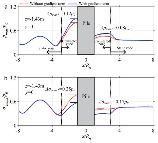
Figure 12.
The discrepancy in (a) the pore pressure and (b) the soil effective stresses caused by the soil property gradient term in a non-homogeneous seabed around a mono-pile (in the x-direction, , m).
Figure 13 shows the discrepancy in (a) the pore pressure and (b) the soil effective stresses caused by the soil property gradient term in a non-homogeneous seabed around a mono-pile (in the y-direction, , m). In contrast to Figure 12, the distribution of pore pressure (p) and soil effective stresses () is found to be symmetric about the middle line of the pile (y = 0). This is because the dynamic wave pressure behaves symmetrically at the sides (in the y-direction) of the pile. Consequently, this generates symmetry in the discrepancy of the pore pressure () and the soil effective stresses (), indicating that the effect of the gradient term on the soil dynamic response is also symmetric. Figure 13 also illustrates that the maximum discrepancy in the soil effective stresses () is , which is larger than that of . This indicates that the distribution gradient of the soil properties has a more significant influence on the soil effective stresses at the sides of the pile (y-direction).

Figure 13.
The discrepancy in (a) the pore pressure and (b) the soil effective stresses caused by the soil property gradient term in a non-homogeneous seabed around a mono-pile (in the y-direction, , m).
Figure 14 further illustrates the discrepancy in (a) the pore pressure and (b) the soil effective stresses caused by the soil property gradient term in a non-homogeneous seabed around a mono-pile (in the z-direction, m, ). Figure 14 shows that the pore pressure (p) decreases from the seabed surface to the deep seabed; this is because of the natural attenuation of pore pressure with increasing seabed depth (Jeng, 2012). The soil effective stresses () are seen to initially increase then decrease quickly when it deepens in the vertical direction. This is because the soil effective stresses are equal to zero at the seabed surface (because there is no compaction of the soil particles) and reach the minimum in the deep seabed (because there is minimal influence from wave loading). Compared with the pore pressure (), the soil effective stresses () are much more affected by the gradient term of the soil property. This is similar to that of Figure 12 (x-direction) and Figure 13 (y-direction), indicating that this conclusion is applicable in the 3D space of a non-homogeneous seabed. In addition, Figure 14 also shows that the maximum discrepancy in the pore pressure () and the soil effective stresses () occurs around the interface (the dashed line) between the convected zone and the static zone. This is perhaps because the soil properties change considerably (large gradient term) at the interface, and it indicates that the property distribution gradient has the largest effect on the seabed response in that location in the vertical direction.
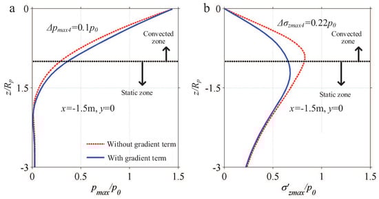
Figure 14.
The discrepancy in (a) the pore pressure and (b) the soil effective stresses caused by the soil property gradient term in a non-homogeneous seabed around a mono-pile (in the z-direction, m, ).
5. Liquefaction
Liquefaction occurs if the excess pore-water pressure exceeds the overburden soil weight. This leads to the disappearance of soil effective stresses, thus potentially causing seabed instability around marine structures. In this section, the effects of the soil distribution gradient on the liquefaction depth are investigated. Parametric studies with various soil and wave parameters are also presented to examine the importance of the distribution gradient terms. For simplicity, the 2D propagating wave cases are adopted when the linear wave theory is used. The liquefaction criterion can be expressed as
where is the submerged weight of the soil.
Figure 15 illustrates the comparison of the liquefaction depth between cases with (solid line) and without (dashed line) the distribution gradient terms of non-homogeneous soil properties. The curves are the values of ; thus, the liquefaction depth can be denoted by the interaction points between the curve () and the vertical line of . It can be observed that the seabed can be liquefied around the seabed surface ( m). The liquefaction depth with the distribution gradient terms ( m) is larger than that without the distribution gradient terms ( m). The present numerical results indicate that common approaches that neglect the distribution gradient terms will underestimate the liquefaction of a non-homogeneous seabed.
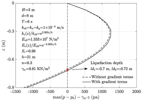
Figure 15.
Comparison of non-homogeneous seabed liquefaction between cases with (solid line) and without (dashed line) distribution gradient terms of non-homogeneous soil properties.
Parametric studies on the importance of the distribution terms are illustrated in Figure 16. The non-dimensional ratio of is adopted as the indicator of the degree of importance, which is plotted with various wave and seabed parameters. It is found that the ratio increases with increasing wave height (H) and decreasing wave period (T) and water depth (d). It does not notably change with the degree of saturation (). This indicates that the effects of the distribution gradient terms will be more pronounced with larger wave heights, lower wave periods, and lower water depth.
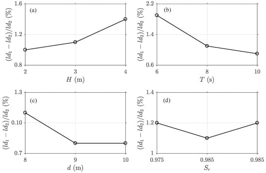
Figure 16.
Parametric studies on the importance of the distribution terms to the liquefaction depth with various (a) wave heights H ( s, m, ), (b) wave periods T ( m, m, ), (c) water depths d ( m, s, ), and (d) degree of saturation ( m. s, m) (the other parameters are found in Figure 15).
It should be noted that, the above discussions on the liquefaction are called the “potential liquefaction”, which means the prediction of the possible maximum liquefaction depth that can be reached with the wave loadings. These are based on the assumption of the static elastic porous seabed. Qi and Gao [42] noted that the seabed liquefaction would shift downward the interface between the seabed and fluid, thus decreasing the liquefaction depth. This means the liquefaction depth predicted in this study is conservative to the engineering practice. Similar research and assumptions can be extensively seen in the previous studies [4,19,32,43]. The simulations on the soil behaviour after the real liquefaction moment may need more sophisticated models, which would be considered in our future studies.
6. Discussion
The distribution gradient of soil properties naturally exists in the governing equations for the wave-induced non-homogeneous seabed response (Equations (21)–(27)). Most previous studies [28,29] have neglected the soil distribution gradient terms by simply adopting the assumption of a layered seabed. A few studies [30,33] considered the gradient terms when simulating the non-homogeneous seabed response; however, the corresponding effect was not quantitatively investigated. The study herein fills this gap by carefully examining the effect of the distribution gradient of soil properties on the dynamic response of a non-homogeneous seabed.
The distributions of the pore pressure (p) and the effective stresses () with and without the property gradient terms are simulated for nine cases () of a 2D non-homogeneous seabed. Results show that the pore pressure (the soil effective stresses) decreases (increase) if the soil distribution gradient term is neglected (see Figure 4 and Figure 6). A large discrepancy in the pore pressure and large soil effective stresses due to the property gradient term occur respectively at the upper seabed and the lower seabed. This means that the largest effect of the property distribution gradient takes place at the upper part of the seabed for the pore pressure, while the largest effect appears at the lower part of the seabed for the soil effective stresses. In addition, pore pressure significantly changes as a result of the change in the permeability gradient (Figure 5), while soil effective stresses significantly change as a result of the change in the Young’s modulus gradient (Figure 7). This indicates that the soil effective stresses and the pore pressure are more sensitive to the distribution gradient of the soil Young’s modulus and permeability, respectively. The maximum discrepancy in the soil effective stresses caused by the soil distribution gradient is about (see Figure 8), indicating that the property distribution gradient cannot be neglected in the governing equations, especially for cases in which the soil effective stresses are the main concern.
The discrepancy in the pore pressure and the soil effective stresses caused by the soil property distribution gradient is investigated for the 3D non-homogeneous seabed around a mono-pile foundation (Figure 9, Figure 10, Figure 11, Figure 12, Figure 13 and Figure 14). The wave reflection and diffraction phenomenon is considered in the vicinity of the mono-pile. It is found that the conclusions obtained from the 2D case cab be extended to the 3D case of the non-homogeneous seabed around the mono-pile. In spite of this, the effect of the soil property distribution gradient on the non-homogeneous seabed response is found to be significantly affected by wave transformations around the pile. The discrepancy in the pore pressures and the soil effective stresses caused by the property distribution gradient is larger in front of the pile than at the rear of the pile. This is because the relatively large wave loading occurs in front of the pile. In addition, a large discrepancy in the seabed variables (i.e., the pore pressure and the soil effective stresses) are found at the convected/static zone interface within the 3D non-homogeneous seabed, indicating that this location is much more influenced by the property distribution gradient than the other part.
Effects of the soil distribution gradient on the liquefaction are also examined in this study. It is found that the liquefaction depth can be underestimated if the distribution gradient terms are neglected. However, it has to be acknowledged that the discrepancy in the liquefaction depth due to the gradient terms are within . This is because the liquefaction occurs at the seabed surface, where there are minor discrepancies of pore pressure caused by the gradient terms (see Figure 4). Therefore, the distribution gradient terms can be neglected in the evaluation of liquefaction in engineering practice.
7. Conclusions
Using a 3D Fully Dynamic (FD) seabed model, this study numerically investigated the effect of the soil property distribution gradient on the non-homogeneous seabed response by adding the gradient terms to the governing equations. The model was well validated by comparing results with available experimental and field measurements. A 2D vertical non-homogeneous seabed case and a 3D non-homogeneous seabed case around a mono-pile were simulated to evaluate the effect of the soil property distribution gradient in different environmental situations. The following conclusions can be drawn:
(1) The pore pressure will decrease while the soil effective stresses will increase if the gradient term of non-homogeneous soil properties is neglected. This influence is much more remarkable for the soil effective stresses, for which the maximum discrepancy can reach for the current cases.
(2) The above effects mainly occur at the upper part of the seabed for pore pressure, while they are more pronounced at the lower part of the seabed for soil effective stresses.
(3) For the non-homogeneous seabed around the mono-pile, the largest effect from the soil property distribution gradient is found in front of the pile, which is the result of wave reflection and diffraction. In the vertical direction, it will occur around the interface of the convected/static zone because this is where the largest change in soil properties occurs.
(4) The effects of the soil distribution gradient on liquefaction increase with the increase (decrease) in wave height (wave period and water depth). The above effects cause a discrepancy in the liquefaction depth of less than for a non-homogeneous seabed.
It should be noted that this study only considered soil properties that vary in space. The much more complex cases with time- and space-based non-homogeneous variables need more advanced models, which may be considered in a future study. The main contribution of this study is the clarification of the effects of the soil distribution gradient on the wave-induced response and liquefaction of a non-homogeneous seabed. This study concludes that the soil distribution gradient terms can significantly affect the soil effective stresses, but such effects on the liquefaction depth are limited. This validates the usage of the simplified approach (neglects the gradient terms) in the evaluation of seabed liquefaction; however, it should be attended to carefully when soil effective stresses are involved.
Author Contributions
Conceptualization, methodology and formal analysis, T.S.; Formal analysis, Y.J., Z.W., J.S.; Supervision, C.Z.
Funding
This research was funded by the National Natural Science Foundation (Grant No. 51909076), the Fundamental Research Funds for the Central Universities (2017B15814), the International Postdoctoral Exchange Fellowship Program (20170014), the National Natural Science Foundation (Grant No. 41706087; Grant No. 51879096), the National Science Fund for Distinguished Young Scholars (Grant No. 51425901), Natural Science Foundation of Jiangsu Province (Grant No. BK20161509), Marine Science and Technology Innovation Project of Jiangsu Province (HY2018-15).
Acknowledgments
The authors thank for the three anonymous reviewers for their critical comments helping us to improve this paper.
Conflicts of Interest
The authors declare no conflict of interest.
References
- Zhang, C.; Zhang, Q.; Zheng, J.; Demirbilek, Z. Parameterization of nearshore wave front slope. Coast. Eng. 2017, 127, 80–87. [Google Scholar] [CrossRef]
- Zheng, J.; Zhang, C.; Demirbilek, Z.; Lin, L. Numerical Study of Sandbar Migration under Wave-Undertow Interaction. J. Waterw. Port Coast. Ocean Eng. 2014, 140, 146–159. [Google Scholar] [CrossRef]
- Zhang, W.; Cao, Y.; Zhu, Y.; Zheng, J.; Ji, X.; Xu, Y.; Wu, Y.; Hoitink, A. Unravelling the causes of tidal asymmetry in deltas. J. Hydrol. 2018, 564, 588–604. [Google Scholar] [CrossRef]
- Sumer, B.M. Liquefaction around Marine Structures; World Scientific: Singapore, 2014. [Google Scholar] [CrossRef]
- Kirca, V.O.; Sumer, B.M.; Fredsøe, J. Residual liquefaction of seabed under standing waves. J. Waterw. Port Coast. Ocean Eng. 2013, 139, 489–501. [Google Scholar] [CrossRef]
- Qi, W.G.; Li, C.F.; Jeng, D.S.; Gao, F.P.; Liang, Z. Combined wave-current induced excess pore-pressure in a sandy seabed: Flume observations and comparisons with theoretical models. Coast. Eng. 2019, 147, 89–98. [Google Scholar] [CrossRef]
- Smith, A.W.; Gordon, A.D. Large breakwater toe failures. J. Waterw. Harbor Coast. Eng. Div. ASCE 1983, 109, 253–255. [Google Scholar] [CrossRef]
- Yamamoto, T.; Koning, H.L.; Sellmeijer, H.; Hijum, E.V. On the response of a poro-elastic bed to water waves. J. Fluid Mech. 1978, 87, 193–206. [Google Scholar] [CrossRef]
- Madsen, O.S. Wave-induced pore pressures and effective stresses in a porous bed. Géotechnique 1978, 28, 377–393. [Google Scholar] [CrossRef]
- Jeng, D.S.; Hsu, J.S.C. Wave-induced soil response in a nearly saturated sea-bed of finite thickness. Géotechnique 1996, 46, 427–440. [Google Scholar] [CrossRef]
- Zienkiewicz, O.C.; Chang, C.T.; Bettess, P. Drained, undrained, consolidating and dynamic behaviour assumptions in soils. Géotechnique 1980, 30, 385–395. [Google Scholar] [CrossRef]
- Jeng, D.S.; Rahman, M.S. Effective stresses in a porous seabed of finite thickness: Inertia effects. Can. Geotech. J. 2000, 37, 1383–1392. [Google Scholar] [CrossRef]
- Ülker, M.B.C.; Rahman, M.S. Response of saturated and nearly saturated porous media: Different formulations and their applicability. Int. J. Numer. Anal. Methods Geomech. 2009, 33, 633–664. [Google Scholar] [CrossRef]
- Liao, C.; Jeng, D.; Lin, Z.; Guo, Y.; Zhang, Q. Wave (Current)-Induced Pore Pressure in Offshore Deposits: A Coupled Finite Element Model. J. Mar. Sci. Eng. 2018, 6, 83. [Google Scholar] [CrossRef]
- Tong, D.; Liao, C.; Chen, J.; Zhang, Q. Numerical Simulation of a Sandy Seabed Response to Water Surface Waves Propagating on Current. J. Mar. Sci. Eng. 2018, 6, 88. [Google Scholar] [CrossRef]
- Chen, W.Y.; Chen, G.X.; Chen, W.; Liao, C.C.; Gao, H.M. Numerical simulation of the nonlinear wave-induced dynamic response of anisotropic poro-elastoplastic seabed. Mar. Georesour. Geotechnol. 2019, 37, 924–935. [Google Scholar] [CrossRef]
- Dunn, S.L.; Vun, P.L.; Chan, A.H.C.; Damgaard, J.S. Numerical Modeling of Wave-Induced Liquefaction around Pipelines. J. Waterw. Port Coast. Ocean Eng. 2006, 132, 276–288. [Google Scholar] [CrossRef]
- Hur, D.S.; Kim, C.H.; Kim, D.S.; Yoon, J.S. Simulation of the nonlinear dynamic interactions between waves, a submerged breakwater and the seabed. Ocean Eng. 2008, 35, 511–522. [Google Scholar] [CrossRef]
- Ye, J.; Jeng, D.; Liu, P.F.; Chan, A.; Wang, R.; Zhu, C. Breaking wave-induced response of composite breakwater and liquefaction in seabed foundation. Coast. Eng. 2014, 85, 72–86. [Google Scholar] [CrossRef]
- Elsafti, H.; Oumeraci, H. A numerical hydro-geotechnical model for marine gravity structures. Comput. Geotech. 2016, 79, 105–129. [Google Scholar] [CrossRef]
- Zhang, J.S.; Jeng, D.S.; Liu, P.L.F. Numerical study for waves propagating over a porous seabed around a submerged permeable breakwater: PORO-WSSI II model. Ocean Eng. 2011, 38, 954–966. [Google Scholar] [CrossRef]
- Liao, C.; Tong, D.; Jeng, D.S.; Zhao, H. Numerical study for wave-induced oscillatory pore pressures and liquefaction around impermeable slope breakwater heads. Ocean Eng. 2018, 157, 364–375. [Google Scholar] [CrossRef]
- Sui, T.; Zhang, C.; Guo, Y.; Zheng, J.; Jeng, D.; Zhang, J.; Zhang, W. Three-dimensional numerical model for wave-induced seabed response around mono-pile. Ships Offshore Struct. 2016, 11, 667–678. [Google Scholar] [CrossRef]
- Sui, T.; Zheng, J.; Zhang, C.; Jeng, D.S.; Zhang, J.; Guo, Y.; He, R. Consolidation of unsaturated seabed around an inserted pile foundation and its effects on the wave-induced momentary liquefaction. Ocean Eng. 2017, 131, 308–321. [Google Scholar] [CrossRef]
- Bennett, R.H.; Faris, J.R. Ambient and dynamic pore pressures in fine-grained submarine sediments: Mississippi Delta. Appl. Ocean Res. 1979, 1, 115–123. [Google Scholar] [CrossRef]
- Yamamoto, T. Wave-induced pore pressures and effective stresses in inhomogeneous seabed foundations. Ocean Eng. 1981, 8, 1–16. [Google Scholar] [CrossRef]
- Rahman, M.; El-Zahaby, K.; Booker, J. A semi-analytical method for the wave-induced seabed response. Int. J. Numer. Anal. Methods Geomech. 1994, 18, 213–236. [Google Scholar] [CrossRef]
- Zhou, X.L.; Xu, B.; Wang, J.H.; Li, Y.L. An analytical solution for wave-induced seabed response in a multi-layered poro-elastic seabed. Ocean Eng. 2011, 38, 119–129. [Google Scholar] [CrossRef]
- Ülker, M.B.C. Semianalytical Solution to the Wave-Induced Dynamic Response of Saturated Layered Porous Media. J. Waterw. Port Coast. Ocean Eng. 2015, 141, 06014001. [Google Scholar] [CrossRef]
- Jeng, D.S.; Lin, Y.S. Finite element modelling for water waves-soil interaction. Soil Dyn. Earthq. Eng. 1996, 15, 283–300. [Google Scholar] [CrossRef]
- Zhang, L.; Cheng, Y.; Li, J.; Zhou, X.; Jeng, D.; Peng, X. Wave-induced oscillatory response in a randomly heterogeneous porous seabed. Ocean Eng. 2016, 111, 116–127. [Google Scholar] [CrossRef]
- Chen, L.; Jeng, D.S.; Liao, C.; Tong, D. Wave-Induced Seabed Response around a Dumbbell Cofferdam in Non-Homogeneous Anisotropic Seabed. J. Mar. Sci. Eng. 2019, 7, 189. [Google Scholar] [CrossRef]
- Zhang, C.; Sui, T.; Zheng, J.; Xie, M.; Nguyen, V.T. Modelling wave-induced 3D non-homogeneous seabed response. Appl. Ocean Res. 2016, 61, 101–114. [Google Scholar] [CrossRef]
- Maeno, Y.; Hasegawa, T. Evaluation of Wave-Induced Pore Pressure in Sand Layer by Wave Steepness. Coast. Eng. Jpn. 1985, 28, 31–44. [Google Scholar] [CrossRef]
- Pickering, D. Anisotropic elastic parameters for soil. Géotechnique 1970, 20, 271–276. [Google Scholar] [CrossRef]
- FUNWAVE 2.0 Fully Nonlinear Boussinesq Wave Model on Curvilinear Coordinates; Research Report CACR-03-xx; University of Delaware: Newark, DE, USA, 2003.
- Wei, G.; Kirby, J.T.; Grilli, S.T.; Subramanya, R. A fully nonlinear Boussinesq model for surface waves. Part 1. Highly nonlinear unsteady waves. J. Fluid Mech. 1995, 294, 71–92. [Google Scholar] [CrossRef]
- Jeng, D.S. Porous Models for Wave-Seabed Interactions; Springer Science & Business Media: Berlin/Heidelberg, Germany, 2012. [Google Scholar] [CrossRef]
- Bennett, R.H.; Li, H.; Lambert, D.N.; Fischer, K.M.; Walter, D.J.; Hickox, C.E.; Hulbert, M.H.; Yamamoto, T.; Badiey, M. In situ porosity and permeability of selected carbonate sediment: Great Bahama Bank Part 1: Measurements. Mar. Georesour. Geotechnol. 1990, 9, 1–28. [Google Scholar] [CrossRef]
- Brown, D.A.; Morrison, C.; Reese, L.C. Lateral load behavior of pile group in sand. J. Geotech. Eng. 1988, 114, 1261–1276. [Google Scholar] [CrossRef]
- Cuéllar, P.; Georgi, S.; Baeßler, M.; Rücker, W. On the quasi-static granular convective flow and sand densification around pile foundations under cyclic lateral loading. Granul. Matter 2012, 14, 11–25. [Google Scholar] [CrossRef]
- Qi, W.G.; Gao, F.P. Wave induced instantaneously-liquefied soil depth in a non-cohesive seabed. Ocean Eng. 2018, 153, 412–423. [Google Scholar] [CrossRef]
- Jeng, D.S.; Ye, J.H.; Zhang, J.S.; Liu, P.L.F. An integrated model for the wave-induced seabed response around marine structures: Model verifications and applications. Coast. Eng. 2013, 72, 1–19. [Google Scholar] [CrossRef]


© 2019 by the authors. Licensee MDPI, Basel, Switzerland. This article is an open access article distributed under the terms and conditions of the Creative Commons Attribution (CC BY) license (http://creativecommons.org/licenses/by/4.0/).