Abstract
In this paper, a model for dynamic analysis of array of floating breakwaters is developed and tested. Special attention is given to modeling connections between neighboring elements of the array. A linear three-dimensional floating multi-body formulation is used as a foundation for the presented model. An additional stiffness matrix is derived which introduces the influence of the connections onto motion of the array. The stiffness matrix is used to couple motions in vertical and horizontal planes i.e., the connections are modeled in three-dimensions. The equation of motion is solved in the frequency domain. The newly developed model is tested on an array of three connected breakwaters. The motion and the performance of the breakwater array are investigated under different significant heights and directions of the incoming waves.
1. Introduction
A port or a marina, as part of the sea water area that is intended for safe keeping of vessels, is normally exposed to significant wave loads. The waves can damage vessels inside, as well as port facilities such as berths or mooring equipment. In order to establish protection against waves, breakwaters are often used.
Nowadays it is common for large ports to be built in areas of relatively high sea depths where bottom founded breakwaters cause difficulties in construction and increase the cost of the installation. For this reason, floating breakwaters are frequently used due to their relatively cheap construction. This kind of breakwaters has been proven to be efficient in providing shelter from waves regardless of the sea depth, tidal variations, and the seabed conditions. The physical rationale for using floating breakwaters is that, according to the usual wave theories, most of the wave energy can be found at the free surface or nearby i.e., at the same location where the breakwaters are installed.
The main characteristic of every breakwater is the wave attenuation that is obtained in the protected area. The attenuation can be achieved by different physical mechanisms. One such mechanism is the reflection of the incoming waves on the vertical sides of floating breakwaters [1]. In contrast, the wave breaking approach is based on the dissipation of the incident wave energy on the inclined surfaces of the breakwater (imitating beach inclination) and it is the most common approach used in the bottom fixed breakwater design [2]. Furthermore, there are friction type breakwaters that disturb wave particle orbits and reduce flow velocity through its submerged parts. These submerged parts are typically frame structures added to the floating parts of the breakwater.
Numerical models for the analysis of breakwater dynamics and their wave attenuation performance are as diverse as their design. In the following, only those models are considered that include connections (hinges) within the structure of the breakwater, and in which these connections play an important role in the response and the efficiency of the breakwater. A representation of connected floating breakwaters can be found in Figure 1 and Figure 2. Hinges are used in a special type of breakwater that resembles the tethered breakwater [3]. The floater is tied to the seabed directly by the hinge. The floater itself is in the form of a vertical plate forming a kind of a wave barrier. Similar to the conventional tethered breakwater design, this special type also moves like an inverted swinging pendulum. Additional mooring lines are installed sideways to increase the restoring moment of the breakwater. The fluid dynamics can be modeled by using linearized potential flow theory (in two dimensions) in combination with boundary value approach [3]. The hinge can be modeled as an additional kinematic condition. The motion of the breakwater is modeled simply as rotation around the hinge (translation displacements are not permitted). The developed model is solved in the frequency domain [3].
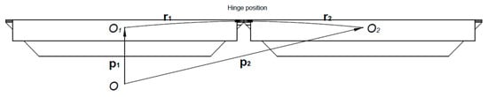
Figure 1.
The connected breakwaters in the initial position.
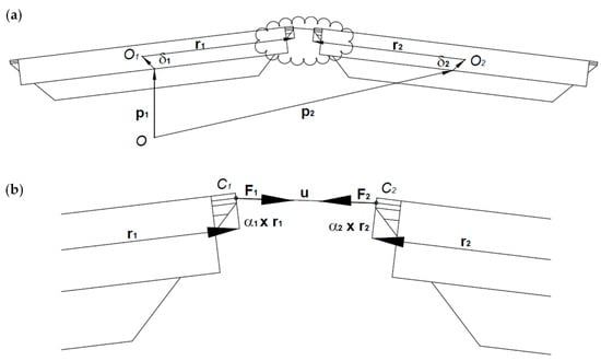
Figure 2.
The connected breakwaters at some time instant: (a) The side view of the connected breakwaters; (b) The zoomed view of the connection.
A (single) deformable body model can be used to analyze dynamics of an array of connected floating breakwaters [4]. This model has been developed by extension of the frequency domain model used for the analysis of motions of a rigid three-dimensional floating body through wave radiation and diffraction. The model considers continuous structural deflections as well as discontinuous deflections that can be used for modeling interactions of multiple floating bodies. A deformable body deflection (under wave loads) is defined by an expansion of chosen modal shape functions and afterwards the response in each mode is evaluated. A similar approach can be found in forced vibration analyses of elastic structures by the modal decomposition technique. In case of separated (rigid) floating bodies that are connected mechanically (by hinges), a special set of shape functions is chosen, the so-called hinge modes that are appropriate for such a discontinuous structure [5]. A hinge mode can be defined as a triangular elevation of two neighboring breakwaters [6], the so called tent function, while other breakwaters are kept at zero elevation. Here, the top the triangle (or the top of the tent) is set at the hinge that connects the two neighboring breakwaters. The total number of hinge modes equals to the number of the hinge connections. The described approach is capable of further extension i.e., incorporation of mooring lines as an additional stiffness in the breakwater installation [7].
Floating breakwaters are rarely made as a single construction. Usually, arrays of breakwater elements of some type are connected together around a sheltered area. These connections certainly affect the motions and effectiveness of the breakwater and thus are important part of the breakwater design. Therefore, it is useful to develop mathematical (and numerical) models that could treat a number of connected floating breakwaters.
In this study, a multi-body model for dynamic analysis of a floating breakwater array is developed. A box-type floating breakwater is considered. Each element in the array of connected breakwaters is considered as a single rigid three-dimensional body. The starting point for the development of the model is the equation of motion of floating bodies that is based on the linearized radiation/diffraction potential theory [8,9]. Hydrodynamic reactions (added mass and radiation damping) are evaluated, and all bodies i.e., mutual hydrodynamic influence of different bodies, are taken into account. Restoring forces are modeled through the global stiffness matrix. Usually, the global stiffness matrix is composed of local stiffness matrices for each floating body that are evaluated through hydrostatic calculations. Such a stiffness matrix would result in uncoupled motions of the breakwater array (at least from the standpoint of restoring forces). In this study, however, the global stiffness matrix is supplemented with additional stiffness matrices for every connection within the breakwater. Therefore, a fully coupled model of all elements in the array of connected floating breakwaters is developed i.e., motions of the array of floating breakwaters with connections can be considered within the hydrodynamic analysis.
2. Overview of the Floating Breakwater Designs
There are several types of floating breakwaters available at the market, which primarily differ in their shape and the physical mechanism(s) responsible for the wave attenuation [10]. In the cases with long waves, floating breakwaters are found to be relatively inefficient in comparison to their bottom mounted counterparts. Different types (or forms) of floating breakwaters are therefore developed to resolve this deficiency. Overall, seven main types can be found in the literature [11], which are shortly described in the following text. Graphical schemes, depictions, and a critical comparison of different types of floating breakwaters can be found in reference [10].
Traditional breakwater types usually rely on one of the three physical mechanisms for reducing waves described in the introduction. For example, box-type and pontoon-type breakwater have vertical sides and therefore reflect the incoming waves [12,13]. In some studies, an improvement of the pontoon-type breakwater is proposed, which consists of converting the space between pontoons into an air chamber. The tuning of the air pressure within the chamber is then used to adjust the resonant period of the breakwater [14]. Another approach is to use the nozzle outlet (on top of the air chamber) in order to achieve pneumatic damping [15].
A modern approach in the breakwater design is to use and combine different mechanisms for wave attenuation. These combinations arise quite naturally, since on any floating body, all of the described mechanisms of wave attenuation can be observed. For example, the frame type breakwater consists of pontoons onto which submerged frames are attached. Concrete pontoons (that usually cause a reflection of incoming waves) are additionally equipped with submerged porous treated timber fences. These fences are installed on either side of the pontoons in order to disturb the wave particle orbits [16]. Cylindrical floating breakwaters are made of rigid cylinders equipped with a flexible mesh cage containing a number of suspended balls. By using this approach, the attenuation of long waves is significantly improved by the attached mesh, [17].
The development of mat-type breakwaters is primarily inspired by using recycled materials in order to obtain a cost-effective product, rather than just by improving the wave attenuation. For example, used car tires can be employed as the main construction element in a cost-effective breakwater [11]. In this design, the tires are connected with high-strength rope or cable in a nearly rigid mat where neighboring tires move relatively little with respect to each other [18]. In the modular design, [19], tire bundles are connected to form a flexible mat i.e., to form a kind of a flexible wave-maze. The pipe-tire floating breakwater [20], utilizes rigid steel tubes that are interleaved into tire arrays in such a way that only flexible rubber connections exist between the tire mazes and the steel tubes. The mat-types are not necessarily constructed from tires, as PVC circular tubes can be used as well [21]. In general, this breakwater type uses friction between the floaters and the sea water in order to dissipate the wave energy. Therefore, the width of the breakwater has to be relatively large in comparison to the incoming wave length.
Horizontal plate type breakwater can be comprehended as an elastic coating of the sea surface. In this design, besides the breakwater dimensions, an important role in the wave attenuation is played by the rigidity of the plate along with its boundary conditions [22]. Perforated i.e., porous plates are used in order to reduce wave forces acting on the breakwater along with the reduction of the plate deflection. Furthermore, porous plates achieve better wave dissipation [23]. The effectiveness of this breakwater type can be improved by adding nets beneath the plate [24]. These nets can also reduce the current velocity which in some cases is beneficial. A special variation in the design of horizontal plate breakwaters is the sub-plate breakwater that dissipates waves by suppressing the wave particle orbits in the vertical direction along with wave breaking on plate edges [25].
The tethered type of floating breakwaters comprises an array of floaters that are tethered to the seabed by individual strings i.e., mooring lines [26]. These floaters are held submerged (or partly submerged) by some kind of ballast units. Generally, the characteristic dimension of the floater is designed to be equal to the wave height. The floaters are usually spherical. Each floater has its own ballast unit which is designed with excess mass that ensures that the ballast rests on the seabed. In another version, the ballast units can be joined together in one large unit that is positioned above the sea bottom with mooring lines and anchors [27]. In all versions, the floater moves periodically (like an inverted swinging pendulum) due to the incoming waves. The dominant attenuation mechanism is the drag (friction) resulting from the floater relative motion i.e., the relative velocity with respect to the fluid particles [28]. The relative velocity of the floater is high for long waves so that this type of breakwater is effective in attenuating long waves [29].
3. Mathematical Model
3.1. Multi-Body Hydrodynamics
The hydrodynamics of bodies in close proximity i.e., multi-body hydrodynamics modeling technique has been developed in the past, primarily to meet the needs of offshore oil and gas industry. A typical task is the determination of relative motions of LNG-FPSO (Liquid Natural Gas Floating Production Storage and Offloading) and a side-by-side positioned LNG carrier taking into account hydrodynamic interactions of the vessels under analysis [8] along with the influence of the mooring system [9].
The response of a single floating body to incoming waves is generally expressed by
where is the mass matrix of the body due to its own mass while is the added mass matrix. Letter i is used for imaginary unit. Hydrostatic stiffness is presented by matrix and matrix is the radiational damping matrix. The first order wave forces are given by vector . The equation is based on the linearized radiation/diffraction potential theory. It is normally solved in the frequency domain for a given incoming wave frequency ω in order to obtain the (complex) amplitude of the body motions {δ }. In Equation (1) there are 6 (complex) equations corresponding to the six degrees of freedom (6 DOF) of a single body. Thus, all matrices are of size of 6×6 and the two vectors are of size of 6×1.
The multi-body problem can be also solved by using Equation (1). However, the overall number of equations is then increased to 6N where N is the number of bodies having 6 DOF each. Consequently, the size of matrices is increased to 6N×6N and the size of vectors increases to 6N × 1. The linearized radiation/diffraction potential theory may still be used. The added mass matrix and the damping matrix are obtained considering all the bodies in order to ensure that hydrodynamic coupling (between the bodies) is achieved. Similarly, the force vector is obtained considering the mutual influence of all the bodies. Only the hydrostatic stiffness matrix is evaluated in an uncoupled manner since the hydrostatic forces are individual for each body. Finally, motions of the multi-body system are obtained in the frequency domain (just as for the single body) and the overall amplitude vector {δ } is calculated, which contains complex amplitudes of motions of all the bodies in 6 DOF.
3.2. The Connection Model
The connection between two floating breakwaters can be understood as a stiffness force (i.e., restoring force). The connection itself has a negligible mass, so that inertial forces due to the connection structure can be ignored. As for the damping forces, they may occur due to the relative velocity with respect to the surrounding fluid or due to the intrinsic damping of the material used. However, since the connection is characterized by relatively small dimensions, the damping forces are also negligible, as can be seen in Figure 1. The forces at the connection are dependent of the displacements of the observed bodies (where displacements of one breakwater influences the displacements of the whole array of connected breakwaters). Therefore, Equation (1) must be extended from the standpoint of the stiffness forces. More precisely, the hydrostatic stiffness matrix must be supplemented with an additional stiffness matrix for each connection.
In order to formulate the additional stiffness matrix it is necessary to define a connection point, where the connection with another breakwater is made. In Figure 2, C1 and C2 are the connection points attached to the first breakwater and the second breakwater, respectively. Letter O represents a (global) stationary reference point while O1 and O2 are the reference points attached to the breakwaters. All considerations are done in a Cartesian three-dimensional coordinate system so the Cartesian vector notation with bold font is used. In Figure 1 the breakwaters are presented in the initial state without any displacements. Vector is a position vector of point O1 with respect to point O and point C1 is defined by the vector (with respect to point O1). These vectors are defined in the initial state and are thus constant in time. An analogous description is valid for vectors and . Points C1 and C2 are at the same position in the initial state, so that the relationship of the position vectors can be formulated as
At some instant of time, the breakwaters will be moved by waves so that the position of the connection points will change. Figure 2 shows the relative position of the connection points denoted by the vector . The translational and rotational displacements of the first breakwater are given by vectors δ1 and , respectively. The denotations and are related to the second breakwater. By the vector analysis and by Figure 2 the following expression is obtained
and simplified by using Equation (2) to the form
where is used to denote the cross product. Equation (4) brings into relation the displacements of the neighboring breakwaters and the relative position of their connection points.
Equation (4) describes the kinematics of the observed problem set, but to fully develop a useful connection model, it is necessary to observe the dynamics. For this purpose, the connection itself can be assumed as a linear spring. The forces exerted at the ends of the spring can formulated as
where is the stiffness coefficient of the spring, assumed to be a constant scalar value i.e., the connection stiffness. Force acts on the first breakwater trough the point C1. Likewise, the force is exerted on the second breakwater. These forces generate moments on the breakwaters with respect to associated reference points O1 and O2, as follows
where the terms in the brackets are the levers, as can be seen in Figure 2.
The above equations can be written in a concise form as follows:
With
And
where T stands for transposal of a vector or a matrix. Vector denotes the connection forces and has the size of 12×1. Vector is of the same size containing displacements of the connected breakwaters. Matrix is represented schematically (i.e., not in rigorous matrix notation) as
where (the dots) represent proper position of the translational or the rotational displacements (to be in consistency with the cross product rule). The obtained matrix has the size of 12×12 and relates the displacements and the connection forces. During the formulation of Equation (12), the non-linear terms are neglected since Equation (1) is linear and solved in the frequency domain [30]. In models were the non-linear terms are included, the motions equation is solved in the time domain [31,32].
Connection forces can be comprehended as external forces acting to the neighboring breakwaters. Therefore, vector is added at the right-hand side of the Equation (1). By moving it to the left-hand side, the final form of the additional stiffness matrix for connection is obtained as
with substitutions
and
where is the identity matrix of size 3×3. Here, denotations , and are used for the components of vector . The same analogy is applied for vector .
It should be noted that vector in Equation (1) has the size 6N×1 where N is an arbitrary number of bodies while the vector of connection forces is size 12×1 since it only incorporates forces and moment between two adjacent bodies. Similarly, matrix has the size 6N×6N while the connection force matrix has a size of 12×12. Therefore some attention is needed, but nothing out of ordinary, when matrix is supplemented with matrix . The proper position of adding the matrix is defined by the displacements amplitude vector {δ } from Equation (1) which contains the displacements amplitudes of all floating breakwaters in the array. The same procedure is used when forming the global stiffness matrix of a structure and performing structural analysis by using the finite element method.
4. Case Studies
The case studies are conducted with three generic (identical) breakwaters connected in one array. The main properties of one breakwater are presented in Table 1. Irregular waves are assumed with significant wave heights of 1.1 m, 1.2 m and 1.3 m. Two incoming wave directions are examined: 60° and 90° (beam waves). The sea depth is set to 8 m. The Tabain wave spectrum [33], specific for the Adriatic sea, is used along with the JONSWAP spectrum. The Tabain spectrum is based on only one parameter, the significant wave height, while the the JONSWAP spectrum is also based on the peak period (besides the significant wave height).

Table 1.
The properties of the breakwater.
The calculations are conducted within software application HydroStar [34] which provides the computation of first and second order loads and motions for arbitrary bodies in deep and finite depth waters, with or without forward speed. The software is based on the potential flow theory and 3D boundary element method and it is capable of dealing with multiple floating bodies in the close proximity.
The panel model of the breakwaters is presented in Figure 3. In the first step, the hydrodynamic reactions (added mass and radiation damping) are evaluated, as well as the linear transfer function (LTF) for the first order wave forces. In the next step, the response amplitude operators (RAOs) for each of the three breakwaters are calculated. The viscous damping is set to 5% of the critical damping for the roll motions. In this step, the newly developed additional stiffness matrix, given by Equation (13), is used for each connection as part of the input for the HydroStar. Between neighboring breakwaters, two connections are modeled, so that the overall number of connections is four in two hinges. The value of the connection stiffness k is chosen to be 108 N/m, see Figure 2, which is approximately 100 times higher than the value of the hydrostatic stiffness for heave of one breakwater. The obtained RAOs are presented in Figure 4. Each graph contains results for all three elements of the breakwater array in relation to the incoming wave direction. Exact position of the elements is shown in Figure 3. Graphical representation of the incoming wave direction can be found in Figure 5. The mooring lines are omitted for the sake of simplicity. In general, a mooring system is used for position keeping of floating breakwaters. It is not intended to influence the first order motions. In this study one of the main concerns are the first order motions of the breakwaters. The same approach for calculation RAOs of floating breakwaters without mooring lines can be found in reference [6].
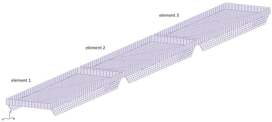
Figure 3.
The panel model of the breakwaters array.
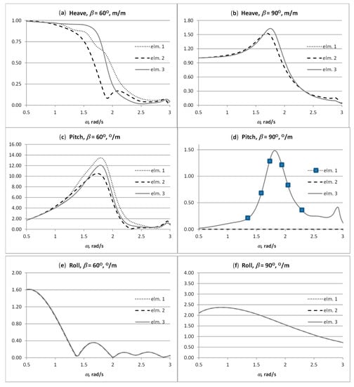
Figure 4.
The response amplitude operators (RAOs) for each of the three breakwaters: (a) Heave for incoming wave direction 60°; (b) Heave for incoming wave direction 90°; (c) Pitch for incoming wave direction 60°; (d) Pitch for incoming wave direction 90°; (e) Roll for incoming wave direction 60°; (f) Roll for incoming wave direction 90°.
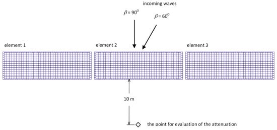
Figure 5.
The position of the point where the attenuation is evaluated.
A part of the case studies is the examination of relative motion of the connection points which belong to one connection between neighboring breakwaters. By using the newly developed mathematical model, the relative motion should be very small in relation to the usual value of the pontoon displacement due to waves. In Figure 2 these points are denoted as C1 and C2. For all four connections, the relative motions RAOs are calculated. It is established that the maximum RAOs value is less than 1 mm. i.e., the numerical results are consistent with the newly developed mathematical model.
Finally, the significant values of the breakwater responses are given in Table 2 regarding the three irregular wave cases.
Table 2.
Significant values of the motions of the breakwaters.
The attenuation AC is evaluated using the expression
where Hs stands for significant wave height of incoming waves while Ht stands for the significant wave height on the sheltered side of the breakwaters. The Ht is calculated based on the RAO for the wave elevation (of the sheltered side) for the point that is set at the side of the breakwaters at a distance of 10 m, see Figure 5. The results are given in Table 3.
Table 3.
Evaluated values of the attenuation.
5. Discussion
The case studies are done with the box-type breakwater. The developed approach is not restricted to this type only. The mathematical model is based on the kinematics of the connection points belonging to two neighboring breakwaters. The dynamics i.e., the forces acting at the connections are modeled with the linear springs. Both of these formulations are quite general and can be used be for any array of connected rigid bodies. Thus, any breakwater type (in an array) that can be assumed to be rigid can be studied using the model for connections developed here. However, the restriction is in the small displacement assumption which is common in models for analyzing breakwaters.
The model is restricted to the stiffness forces only. It is uncoupled from the calculation of the breakwater hydrodynamics. Within the linearized radiation/diffraction potential theory, it does not affect the calculations of the hydrodynamic reactions and the wave loads. As a result, it can be easily used with common seakeeping software that can deal with multi-body problem. This kind of software is readily available, since they are developed (and well matured) during use in the offshore oil and gas industry. Therefore, the additional stiffness matrices for connections are sufficient input to a seakeeping software to examine an array of connected floating breakwaters. Furthermore, this approach can be used for approximating the wave attenuation as demonstrated in the case studies.
As mentioned in the introduction, the problem of connected breakwaters so far has been solved by two approaches. The first approach was presented on the special type of the breakwater in which the floater is tied to the seabed directly by the hinge [3]. The second approach is based on the single deformable body model that is usually used for the hydroelastic analysis of ships [4,5,6,7]. Both of these approaches are developed within the specific mathematical/numerical models. The first approach can only be used for the specific case of a breakwater with only one connection (or hinge). The second approach is quite general when dealing with ship hydroelasticity within the linearized radiation/diffraction potential theory that is solved in the frequency domain. In such an approach, a special type of software is needed that is more complex and advanced than the usual seakeeping software. The newly developed approach presented in this study has a certain advantage for use, because it is based on general assumptions for the kinematics and the dynamics. The additional stiffness matrix for connection can be used in the frequency domain and in the time domain. The hydrodynamics of the multi-bodies do not need to be based on the traditional linearized radiation/diffraction potential theory. The hydrodynamics can be evaluated with some empirical expression or by advanced calculations method like computational fluid dynamics. However, one should keep in mind that the developed model is based on the small displacement assumption.
6. Conclusions
Different types of breakwaters are used for protection against sea waves of a port or a marina. Most of them can be regarded as rigid floating bodies connected in an array around the sheltered area. This study presents the development of a new mathematical model for considering the connections between breakwaters. The connection itself can be understood as additional stiffness forces. Thus the derivation of the additional stiffness matrix that can be used for modeling of one connection is presented.
If the hydrodynamic model is based on the linearized radiation/diffraction potential theory, the usual seakeeping software can be used for the analysis of an array of floating breakwaters connected with hinges. The additional stiffness matrix for each connection is then given as an input to the software. Since the overall model is linear, it is solved in the frequency domain. However, the model for connections developed here is suitable for use in the time domain. Also, it can be used in combination with other methods for solving the hydrodynamics of rigid floating bodies in close proximity.
Future investigations can be aimed at different types of connection i.e., other than hinge. Many types of breakwaters are connected with rubber connections that have significantly less structural stiffness than usual hinges. The difference can also be found in the rubber connection rotational stiffness. A new model should be developed that is able to capture the properties of the rubber connection in order to check the structural integrity of the connection itself (besides the evaluation of the breakwater motions).
Author Contributions
I.Ć. formulated the concept. I.Ć. and M.Ć. conducted formal analysis; I.Ć. and N.A. developed methodology; J.P. provided the resources; I.Ć. conducted software calculations; I.Ć. and N.A. wrote original draft; I.Ć., M.Ć., N.A. and J.P. wrote and edited the paper.
Acknowledgments
The Croatian Science Foundation HRZZ-IP-2016-06-2017 (WESLO) support is gratefully acknowledged.
Conflicts of Interest
The authors declare no conflict of interest.
References
- Sawaragi, T. Coastal Engineering—Waves, Beaches, Wave-structure Interaction, 1st ed.; Elsevier Science: Armsterdam, The Netherlands, 1995. [Google Scholar]
- Carević, D.; Mostečak, H.; Bujak, D.; Lončar, G. Influence of water-level variations on wave transmission through flushing culverts positioned in a breakwater body. J. Waterw. Port Coast. Ocean Eng. 2018, 144, 04018012. [Google Scholar] [CrossRef]
- Leach, P.A. Hinged Floating Breakwater: Theory and Experiments. Master’s Thesis, Oregon State University, Corvallis, OR, USA, 1983. [Google Scholar]
- Newman, J.N. Wave effects on deformable bodies. Appl. Ocean Res. 1994, 16, 47–59. [Google Scholar] [CrossRef]
- Lee, C.H.; Newman, J.N. An assessment of hydroelasticity for very large hinged vessels. J. Fluids Struct. 2000, 14, 957–970. [Google Scholar] [CrossRef]
- Angelides, D.C.; Diamantoulaki, I. Analysis of performance of hinged floating breakwaters. Eng. Struct. 2010, 32, 2407–2423. [Google Scholar]
- Angelides, D.C.; Diamantoulaki, I. Modeling of cable-moored floating breakwaters connected with hinges. Eng. Struct. 2011, 33, 1536–1552. [Google Scholar]
- Kim, M.S.; Ha, M.K.; Kim, B.W. Relative motions between LNG-FPSO and side-by-side positioned LNG carrier in waves. In Proceedings of the Thirteenth International Offshore and Polar Engineering Conference, Honolulu, HI, USA, 25–30 May 2003. [Google Scholar]
- Buchner, B.; van Dijk, A.; de Wilde, J. Numerical multiple-body simulations of side-by-side mooring to an FPSO. In Proceedings of the Eleventh International Offshore and Polar Engineering Conference, Stavanger, Norway, 17–22 June 2001. [Google Scholar]
- Dai, J.; Wang, C.M.; Utsunomiya, T.; Duan, W. Review of recent research and developments on floating breakwaters. Ocean Eng. 2018, 158, 132–151. [Google Scholar] [CrossRef]
- McCartney, B.L. Floating breakwater design. J. Waterw. Port Coast. Ocean Eng. 1985, 111, 304–318. [Google Scholar] [CrossRef]
- Carver, R.D. Floating Breakwater Wave-Attenuation Tests for East Bay Marina, Olympia Harbor, Washington; Technical Report HL-79–13; U.S. Army Engineer Waterways Experiment Station: Vicksburg, MS, USA, 1979. [Google Scholar]
- Nece, R.E.; Richey, E.P. Wave Transmission Tests of Floating Breakwater for Oak Harbor. Water Resources Series; Technical Report No. 32; Department of Civil Engineering, University of Washington: Seattle, DC, USA, 1972. [Google Scholar]
- Ikeno, M.; Shimoda, N.; Iwata, K. A new type of breakwater utilizing air compressibility. In Proceedings of the 21st Coastal Engineering Conference, Torremolinos, Spain, 20–25 June 1988; pp. 2326–2339. [Google Scholar]
- Koo, W. Nonlinear time-domain analysis of motion-restrained pneumatic floating breakwater. Ocean Eng. 2009, 36, 723–731. [Google Scholar] [CrossRef]
- Allyn, N.; Watchorn, E.; Jamieson, W.W.; Yang, G. Port of Brownsville floating breakwater. In Proceedings of the Ports Conference, Norfolk, VA, USA, 29 April–2 May 2001; pp. 1–10. [Google Scholar]
- Ji, C.Y.; Chen, X.; Cui, J.; Yuan, Z.M.; Incecik, A. Experimental study of a new type of floating breakwater. Ocean Eng. 2015, 105, 295–303. [Google Scholar] [CrossRef]
- Candle, R.D. Goodyear scrap tire floating breakwater concepts. In Proceedings of the Floating Breakwaters Conference, Kingston, RI, USA, 23–25 April 1974; pp. 193–212. [Google Scholar]
- Kowalski, T. Scrap tire floating breakwaters. In Proceedings of the Floating Breakwater Conference, Kingston, RI, USA, 23–25 April 1974; pp. 233–246. [Google Scholar]
- Harms, V.W.; Westerink, J.J.; Sorensen, R.M.; McTamany, J.E. Wave Transmission and Mooring-Force Characteristics of Pipe-Tire Floating Breakwaters; Technical Paper 82–84; U.S. Army Coastal Engineering Research Center: Fairfax, VA, USA, 1982. [Google Scholar]
- Hegde, A.V.; Kamath, K.; Magadum, A.S. Performance characteristics of horizontal interlaced multilayer moored floating pipe breakwater. J. Waterw. Port Coast. Ocean Eng. 2007, 133, 275–285. [Google Scholar] [CrossRef]
- Shugan, I.V.; Hwung, H.H.; Yang, R.Y.; Hsu, W.Y. Elastic plate as floating wave breaker in a beach zone. Phys. Wave Phenom. 2012, 20, 199–203. [Google Scholar] [CrossRef]
- Koley, S.; Sahoo, T. Oblique wave scattering by horizontal floating flexible porous membrane. Meccanica 2017, 52, 125–138. [Google Scholar] [CrossRef]
- Dong, G.H.; Zheng, Y.N.; Li, Y.C.; Teng, B.; Guan, C.T.; Lin, D.F. Experiments on wave transmission coefficients of floating breakwaters. Ocean Eng. 2008, 35, 931–938. [Google Scholar] [CrossRef]
- Takaki, M.; Fujikubo, M.; Higo, Y.; Hamada, K.; Kobayashi, M.; Nakagawa, H.; Morishita, S.; Ando, K.; Tanigami, A. A new type VLFS using submerged plates: Sub-plate VLFS. Part 1 Basic concept of system. In Proceedings of the 20th International Conference on Ocean, Rio de Janeiro, Brazil, 3–8 June 2001; pp. 3–8. [Google Scholar]
- Jones, D.B. An Assessment of Transportable Breakwaters with Reference to the Container Off-Loading and Transfer System (COTS); Technical Note No. N-1529; Civil Engineering Laboratory, Naval Construction Battalion Center: Gulfport, MS, USA, 1978. [Google Scholar]
- Hales, L.Z. Floating Breakwater: State-of-the-Art Literature Review; Technical Report No. 81-1; U.S. Army Coastal Engineering Research Center: Fairfax, VA, USA, 1981. [Google Scholar]
- Seymour, R.J.; Hanes, D.M. Performance analysis of tethered float breakwater. J. Waterw. Port Coast. Ocean Eng. 1979, 105, 265–280. [Google Scholar]
- Vethamony, P. Wave attenuation characteristics of a tethered float system. Ocean. Eng. 1995, 22, 111–129. [Google Scholar] [CrossRef]
- Ćatipović, I.; Čorić, V.; Veić, D. Calculation of floating crane natural frequencies based on linearized multibody dynamics equations. In Proceedings of the 30th International Conference on Ocean, Rotterdam, The Netherlands, 19–24 June 2011. [Google Scholar]
- Ćatipović, I.; Čorić, V.; Radanović, J. An improved stiffness model for polyester mooring lines. Brodogradnja 2011, 62, 235–248. [Google Scholar]
- Lyu, B.; Wu, W.; Yao, W.; Wang, Y.; Zhang, Y.; Tang, D.; Yue, Q. Multibody dynamical modeling of the FPSO soft yoke mooring system and prototype validation. Appl. Ocean Res. 2019, 84, 179–191. [Google Scholar] [CrossRef]
- Parunov, J.; Čorak, M.; Pensa, M. Wave height statistics for seakeeping assessment of ships in the Adriatic Sea. Ocean Eng. 2011, 38, 1323–1330. [Google Scholar] [CrossRef]
- Bureau Veritas. HydroStar for Experts—User Manual; Bureau Veritas: Paris, France, 2018. [Google Scholar]


© 2019 by the authors. Licensee MDPI, Basel, Switzerland. This article is an open access article distributed under the terms and conditions of the Creative Commons Attribution (CC BY) license (http://creativecommons.org/licenses/by/4.0/).