Abstract
This paper presents an incremental variational method to assimilate the observed tidal harmonic constants using a frequency domain linearized shallow water equation. A cost function was constructed with tidal boundary conditions and tidal forcing as its control (independent) variables. To minimize the cost function, optimal boundary conditions and tidal forcing were derived using a conventional dual 4-Dimensional Variational (4D-Var) Physical-space Statistical Analysis System. The tangent linear and adjoint model were solved by using a finite element method. By adapting the incremental form, the variational method streamlines the workflow to provide the incremental correction to the boundary conditions and tidal forcing of a hydrodynamic forward model. The method was tested for semi-diurnal M2 tides in a regional sea with a complex tidal system. The results demonstrate a 65–72% reduction of tidal harmonic constant vector error by assimilating the observed M2 tidal harmonic constants. In addition to improving the tides of a hydrodynamic model by optimizing boundary conditions and tidal forcing, the method computes a spatially varying uncertainty of individual tidal constituents in the model. The method provides a versatile tool for mapping the spatially continuous tides and currents in coastal and estuarine waters by assimilating the harmonic constants of individual tidal constituents of observed tides and currents.
1. Introduction
Tidal data assimilation is essential to improve accuracy in a number of important modeling applications in the National Ocean Service (NOS), National Oceanic and Atmospheric Administration (NOAA). For example, Operational Forecast Systems (OFS) are the backbone of the operational coastal ocean forecast system [1] in NOAA’s NOS. Every day, OFSs provide up to 5-day forecasts of water levels, currents, temperature and salinity in US coastal, Great Lakes, and estuarine waters. Until recently, all of NOAA’s operational OFSs were operated in a pure forecast mode without data assimilation. Assimilating observed tides and currents could be considered one of the most urgent agenda items for the next generation of OFSs. Another application is the U.S. national VDatum program in NOAA. The VDatum program has been providing tidal datum products [2] and software to vertically transform geospatial data among a variety of vertical datums, including tidal, orthometric, and ellipsoid-based vertical datums. The program has ongoing projects to upgrade the VDatum products and software. Two of the main goals for the upgrades are to provide spatially varying uncertainty for the VDatum products and to reduce the uncertainty. Tang et al. [3] have shown that the improvement in tide model accuracy can reduce the uncertainty in the tidal datum products. Up to this point, the offshore boundary inputs to the tide model [3] used for VDatum were taken directly from tidal databases without assimilation of tides. Therefore, a tide assimilation scheme is needed to optimize and improve the offshore tidal boundary conditions and the resulting simulation accuracy of the ADCIRC [4] tide modeling for VDatum applications.
Tidal simulations with a hydrodynamic model are usually forced by the predicted tides and tidal currents prescribed at the open boundary, and tidal forcing in the interior of the domain derived from the astronomical tidal potential. The predicted tides and currents consist of the major tidal constituents. In this paper, we would like to propose a methodology to improve the tide and current forecasts in hydrodynamic model by making corrections to the open boundary conditions and tidal forcing by assimilating the harmonic constants of observed tides and currents.
Tides and tidal current dynamic simulations have existed for more than 100 years. One of the early practices was to use the frequency domain model [5] using a linear tidal equation. Taylor [5] demonstrated the mechanisms of a semidiurnal M2 amphidromic system in a rectangular basin, and how the formation and location of the amphidrome(s) are regulated by the bottom friction and physical dimensions of the basin. The frequency domain model has been very successful in simulating the tides [4,6,7,8,9,10]. The biggest success of frequency domain hydrodynamic modeling was to generate a large-scale tidal database by assimilation of satellite altimetry data [7,11,12]. Stammer et al. 2014 [12] provided a very comprehensive review of the status of the tidal database development. These databases [11,12,13] are able to provide highly accurate predicted tides on a global scale (usually within a few centimeters in the open ocean). Even with all the success of the frequency domain tidal modeling in solving the tides by assimilating the observed tidal harmonic constants, the frequency domain data assimilation does not directly address the tides assimilation in real-time forecast models, e.g., 4D-Var Regional Ocean Modeling System (ROMS) [14]. Moore et al. [14] have developed a very mature 4D-Var data assimilation framework for coastal and estuarine waters, but they did not provide any insight into assimilating the tides. In this paper, we would like to address the tides assimilation in time-integrating OFS using a frequency domain model. The layout of the paper is as follows: Section 2 will provide a formulation of the data assimilation of tides and the setup of a test case in the Bohai Sea, Section 3 will present results from the test case of M2 tides in the Bohai Sea, followed by a brief discussion in Section 4, and conclusions in Section 5.
2. Method
This is an incremental variational method to assimilate the observed tidal harmonic constants using a frequency domain linearized shallow water equation. The procedural flow and notation follow Moore et al. 2011 [14] closely.
2.1. Method and Mathematical Formulation
The method is a weak-constraint incremental variational method. For purposes of simplification, we will not write the full linearized shallow water equation; rather, we use operators to represent the dynamic system and projections among control variable space, model state variable space, and observation space [14].
Dynamic system:
where x is the model state variable including water level and depth averaged tidal currents, M is the frequency domain shallow water equation operator [6,7]. is the control variable (or control vector since it is a vector in discrete form, exchangeable throughout the paper) including the boundary condition b, usually prescribed tidal harmonic constants of a tidal harmonic constituent, and forcing term η, at the initial state, the tidal astronomical potential.
x = M(z)
Observation system:
where y is the observed state variable at observation locations, H is the projection operator projecting the model state variable into the observation locations. The combination of Equations (1) and (2) is an overdeterministic system of equations for control variable z. To solve the problem and find an optimal boundary condition and tidal forcing, a cost function J(z) to compromise Equations (1) and (2) is defined as
where z0 is the initial state of the control vector z. D = diag (Bb, Q), the background error covariance of initial control vector z0, where Bb is the boundary condition error covariance matrix, Q is the model potential forcing error covariance matrix. R is the observation error covariance matrix.
y = H(x)
Re-arrange Equation (3) into an incremental formulation, then,
where δz = (z − z0), is the control vector increment, d = y − H(x0), the innovation vector, x0 = M(z0) is the initial model state variable fields. G = HM is the operator that maps from model space to observation space.
The solution to Equation (4) in dual formulation is simple [14]:
In Equation (5), G is the tangent linear model sampled at observation points, and GT is the adjoint model that projects from observation point to the model field. The correction field of control vector δz can be subsequently applied to any linear or non-linear forward hydrodynamic model. The update of the model state variables increment δx will be determined by the forward model.
The solution to the Equation (5) follows the ROMS 4D-Var formulation [14] closely. We adapted the dual 4D-Var Physical-space Statistical Analysis System (PSAS) algorithm [15] (Figure 1), due to the fact that PSAS is conceptually more flexible and computationally more efficient to incorporate the method into a non-linear system (e.g., ADCIRC [4], FVCOM [16], ROMS [14], SCHISM [17]), and to derive useful utilities from the approach, for example spatially varying uncertainty and observation impact and sensitivity assessment.
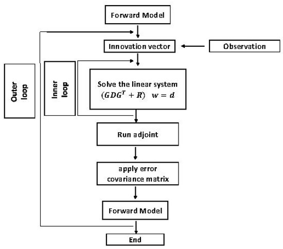
Figure 1.
A flow chart illustrating the data assimilation algorithm.
2.2. Spatially Varying Uncertainty
The posterior control vector is
where , the gain matrix for control vector z. The posterior error covariance matrix of control vector z is
The implied prior error covariance matrix of state variable x is P = MDMT. If the forward model is a linear system, then the posterior error covariance matrix of state variable x is given by
2.3. Test Case in Bohai Sea
Bohai Sea and a linear forward system (linearized shallow water equation) will be used to test the data assimilation algorithm. The Bohai Sea is a shallow semi-enclosed embayment in the northwest Pacific Ocean (Figure 2a). The tidal system in Bohai Sea is very well documented from observations and hydrodynamic model simulations [16,18,19]. The test data set for this case are semidiurnal M2 tidal harmonic constants from 32 tidal stations in the Bohai Sea [16] (Figure 2a). The reason we chose the Bohai Sea is that it has very distinguished and prominent amphidromic system(s) both for diurnal and semi-diurnal tides [16,18,19], which makes it a very good testing ground for the tidal assimilation scheme. The bathymetry data are depth readings from nautical charts. To simulate the tides, an unstructured triangular grid is generated with 26,002 nodes and 49,610 elements (Figure 2b). The tangent linear, adjoint model and linear forward model are solved using finite element method on the unstructured triangular mesh grid.
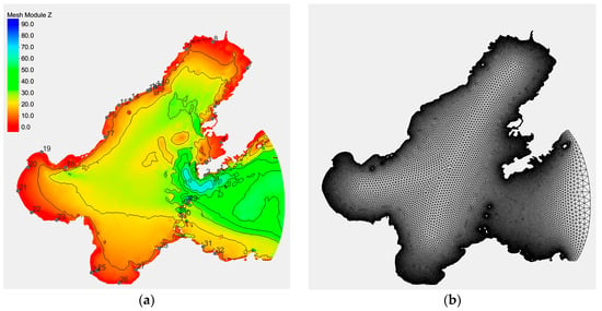
Figure 2.
Bohai Sea model domain (the scale of the domain is about 450 km by 450 km). (a) Bathymetry (m) with colored contour and color bar, and 32 tidal stations (grey dots). (b) unstructured triangular mesh grid (26,002 nodes and 49,610 elements) with 500 m resolution near the shore.
2.4. Test Case Setup
In this test, we use a linearized shallow water equation as the forward model to compute the tides [20]. The model setup is forced either by open boundary conditions only or both open boundary conditions and tidal potential forcing. For tide modeling, there is no background or initial condition of the state variable x (water level, currents). Rather tides/currents are solely determined by the control vector, boundary condition or/and body forcing, as Equation (1) x = M(z) indicates. The importance of astronomical tidal potential in tide modeling is positively correlated with the domain size. Usually the larger the domain, the more important the tidal potential.
To set up the model, we extracted the boundary conditions for the M2 tide from FES2012 [11]. A linear bottom friction was used with a constant bottom friction coefficient. In addition to the hydrodynamic model setup, diagonal elements of all three error covariance matrixes (Bb, Q, R) have to be prescribed. We used a constant 0.1 m error in standard deviation for boundary conditions, and a constant 0.1 m error in standard deviation for tidal forcing. The correlation coefficient is generated with a diffusion operator and a 60 km correlation scale for both [21]. The observation error was 0.03 m without correlation between the stations.
2.5. Experiments
In the next Section, we present the test results in the Bohai Sea. Since there is very limited observational data available from this region, in this experiment, we assimilated all the data available. To evaluate the skill of the data assimilation, we use the delete-1 jackknifing method for error estimate [22]. Specifically, a subsample size of N−1 out of a total of N samples was used, and a total of N repeat samplings were performed by removing one station at a time. At the end, we had N error values, one at each station, and the statistics of the error were calculated. This experiment is designed to quantify the performance of different methods using limited data points at fixed locations without a known reference field.
3. Results
The incremental form of the variational scheme enables the data assimilation to be used for adjustment of boundary conditions and model corrections for linear or non-linear hydrodynamic models in general. The flow chart (Figure 1) indicates that there can be any type of forward hydrodynamic model at the end of the outer loop (within the outer loop). In this paper, we concentrate the application on using a linearized shallow water equation as the forward model. For a hydrodynamic forward model, it will require running the forward model before the outer loop to compute the initial innovation vector, and then computing the posterior state variable x at the end of outer loop.
3.1. Application in the Bohai Sea
Three tests were conducted, (1) test with original boundary condition, (2) test with optimized boundary conditions, (3) test with optimized boundary conditions and tidal forcing correction. Table 1 shows the test results. Both tests (2) and (3) indicate a steady reduction of the water level error in standard deviation (vector difference of the tidal harmonic constants).

Table 1.
M2 tides model error (m) (standard deviation of the model-observation vector difference).
The M2 tides with initial boundary condition (Figure 3) shows two M2 amphidromic systems in the Bohai Sea which are indicated by the small amplitude and circled co-amplitude lines (Figure 3a) and the co-phase lines that rotate around the amphidromic points (Figure 3b). The high amplitude is in the far end of the bay in the north (called north bay thereafter), and the bay in the west (west bay), and the north part of the open boundary. The results show a high discrepancy in both amplitude and phase. The standard deviation of the vector difference with observations is 0.38 m (Table 1). After boundary condition optimization (Figure 4), the error reduces to 0.23 m. The large amplitudes (Figure 4a) at north bay, west bay and open boundary decrease. The phase has the most significant shift, about 30° on average (Figure 4b). If we optimize the boundary condition and make corrections to the tidal forcing, the error further reduces to 0.13 m (Table 1). The amplitude in the west bay and open boundary increase slightly (Figure 5a). The phase has some subtle change, mainly phase reduction (Figure 5b). Amphidromes shift slightly offshore. Overall the pattern is very similar between test case (2) and test case (3).
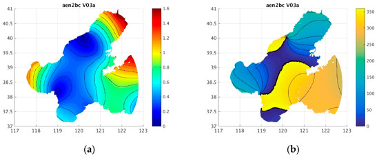
Figure 3.
M2 co-amplitude lines (m) (a) and co-phase lines (o) (b) in the Bohai Sea, generated with initial boundary condition and astronomical forcing.
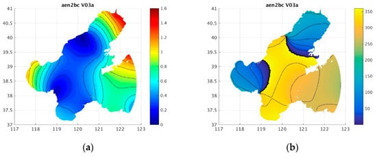
Figure 4.
M2 co-amplitude lines (m) (a) and co-phase lines (o) (b) in Bohai Sea, generated with optimal boundary condition.
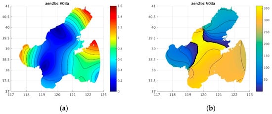
Figure 5.
M2 co-amplitude lines (m) (a) and co-phase lines (o) (b) in Bohai Sea, generated with optimal boundary condition and corrected tidal forcing.
3.2. Spatial Varying Uncertainty
In variational data assimilation, the most challenging part is the background error covariance matrix. To make things more complicated, even after we prescribe the error covariance matrix for control vector, the state variable error covariance matrix still has to be derived. Here, we calculated the uncertainty of state variable x, for the boundary condition only case and the boundary condition plus tidal forcing correction case. Figure 6a is the prior error of the M2 tides for the boundary condition case. The spatial pattern is strikingly similar to the M2 amplitude field (Figure 5a). What can be seen is that wherever there is error on the boundary, the error will propagate into the interior following the dynamics of the Bohai Sea, and naturally will be amplified near the end of the north bay and west bay. Thus, in this particular case, the error for the model state variable is not evenly distributed in space. The error of the state variable is more closely related to the tidal amplitude in the bay. The correction to the boundary condition will drastically reduce the model error, which is evidently shown in the posterior error distribution (Figure 6b). Figure 6b is not the whole picture of the model posterior error after boundary condition optimization, since it assumes a perfect hydrodynamic model. Considering a non-perfect hydrodynamic model, the tidal forcing error will add to the boundary condition uncertainty (Figure 7a). The high prior error of the state variable is most pronounced in the north bay, west bay and the bay in the south. The highest magnitude is about 0.40 m. After assimilating the harmonic constants from 32 stations, the results show a much smaller and spatially evenly distributed posterior error with an average error in standard deviation of about 0.10 m (Figure 7b).
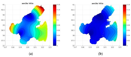
Figure 6.
M2 water level uncertainty field (m) from boundary condition only data assimilation. (a) prior error distribution of the model state variable, water level. (b) posterior error distribution.
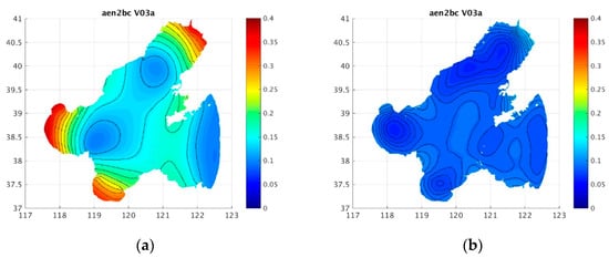
Figure 7.
M2 water level uncertainty field (m) from boundary condition and tidal forcing data assimilation. (a) prior error distribution of the model state variable, water level. (b) posterior error distribution.
4. Discussions
For a hydrodynamic model of a regional sea with an open boundary, open boundary conditions are always the dominant driving force for the tides. There are many studies [9,10,19] that have demonstrated that the boundary condition can be derived from the observed tides within the model domain with good knowledge of the bathymetry without prior knowledge of the initial boundary condition. In the Bohai Sea case, the initial tidal boundary condition can be simply set to zero, and an optimal boundary can be recovered from observed tidal harmonic constants. The boundary condition can converge very quickly in a few (1 or 2) iterations (outer loop, Figure 1).
In this particular case, we use the linear tidal equation as the forward model. For a non-linear hydrodynamic model, one only needs to switch the non-linear model as the forward model in the data assimilation flow chart (Figure 1). Take ADCIRC as an example. The tidal data assimilation work flow sequence will be: run ADCIRC as the forward model using an initial control vector and generate tidal harmonic constants, calculate the innovation vector for individual tidal constituents, calculate the incremental control vector, and use the updated control vector to run ADCIRC. The process can be repeated a few times if needed.
The methodology presented here is essentially a Physical-space Statistical Analysis System (PSAS) [15] that follows the flow chart outlined by Moore et al., 2011 [14]. There are a few parameters for fine tuning within the assimilation scheme, for example the bottom friction coefficient, radius of influence for diffusion operator, and magnitude of error covariance matrix. The accuracy/precision of the forward model is very important. Table 1 also shows the test results with a spatially varying linear bottom friction coefficient that is proportional to the magnitude of the M2 tidal currents. The results show larger improvements as compared to a constant bottom friction coefficient.
In general practice, the incremental formulation will avoid the direct involvement of the baseline simulation which can be a linear or nonlinear forward model. Ideally, for all practical purposes, the non-linear forward model would be a better option. It can account for the non-linearity of the system. Not only is the non-linear bottom friction a better representation of the interaction between the flow and sea bottom, but it also can generate the overtides and compound tides. Sometimes, the overtides and compound tides can be very important. Using the nonlinear forward model would relieve the burden that a linear model has when trying to mimic the mechanism of the nonlinear nature of bottom friction, for the overtides and compound tides generation. With a reasonable spatial distribution of the observation points, the data assimilation algorithm should be able to recover and optimize the overtides and compound tides as well.
5. Conclusions
Tides usually are the most significant factor of variation in water levels and currents in coastal and estuarine waters. For practical and procedural reasons, skill assessment for Operation Forecast System (OFS) is first made for simulations of the tides. This paper presents a generalized framework of an incremental variational data assimilation method to assimilate the tidal harmonic constants into a hydrodynamic model using a frequency domain linearized shallow water equation. The method is capable of providing a correction to the boundary conditions and the model tidal forcing of the hydrodynamic model. In addition, it also provides the spatially varying uncertainty for the tides. The test in the Bohai Sea, a semi-enclosed regional sea with complex amphidromic system(s), demonstrated the capability of the methodology to assimilate the tides and to improve the tidal field. Both tidal amplitude and phase are very smooth without singularities. Overall the method provides a practical/theoretical framework for tidal data assimilation in both NOAA’s Operational Forecast Systems and its National VDatum program, to improve OFS’s skill assessment and to reduce uncertainty in the VDatum products, respectively. In conjunction with a nonlinear hydrodynamic model, e.g., ADCIRC [4], FVCOM [16], ROMS [14], SCHISM [17] etc., it will be able to provide the correction to the boundary condition and tidal potential over a few outer loops. Since the corrected tidal potential or harmonic constants are time-independent, no further tidal data assimilation is needed in the real time integrating forward model run.
The assimilation scheme also quantifies the uncertainty field of tides, which provides utilities for optimizing observation locations, conducting observation impact and observation sensitivity tests, and tidal observing system simulation experiments [14]. The method provides a versatile tool for mapping the spatially continuous tides and currents in coastal and estuarine waters by assimilating the harmonic constants of individual tidal constituents of observed tides and currents. In future work, the methodology will be further tested, validated and applied using a non-linear hydrodynamic model in the context of NOAA’s Operational Forecast Systems and VDatum tidal modal development.
Author Contributions
L.S. and E.M. conceived and designed the methodology and experiments; L.S. and L.T. performed the model development and experiments; L.S., L.T. and E.M. drafted the manuscript. All authors read and approved the final manuscript.
Funding
This research received no external funding.
Acknowledgments
Authors would like to thank NOAA/NOS’ NGS, CO-OPS and OCS VDatum project tri-office management and technical teams’ support of the project. We would also like to thank many experts in and outside of NOAA for going through the project report review process and providing valuable comments and advice to improve the technical report and manuscript.
Conflicts of Interest
The authors declare no conflict of interest.
References
- Zhang, A.; Hess, K.W.; Aikman, F., III. User-based skill assessment techniques for operational hydrodynamic forecast systems. J. Oper. Oceanogr. 2010, 3, 11–24. [Google Scholar] [CrossRef]
- Shi, L.; Myers, E. Statistical Interpolation of Tidal Datums and Computation of Its Associated Spatially Varying Uncertainty. J. Mar. Sci. Eng. 2016, 4, 64. [Google Scholar] [CrossRef]
- Tang, L.; Myers, E.; Shi, L.; Hess, K.; Carisio, A.; Michalski, M.; White, S.; Hoang, C. Tidal Datums with Spatially Varying Uncertainty in North-East Gulf of Mexico for VDatum Application. J. Mar. Sci. Eng. 2018, 6, 114. [Google Scholar] [CrossRef]
- Luettich, R.A.; Westerink, J.J.; Scheffner, N.W. ADCIRC: An Advanced Three-Dimensional Circulation Model for Shelves, Coasts and Estuaries; U.S. Army Eng. Waterw. Exp. Stn.: Vicksburg, MS, USA, 1992. [Google Scholar]
- Taylor, G.L. Tidal Oscillations in Gulf and Rectangular Basins. Proc. Lond. Math. Soc. 1920, 20, 148–181. [Google Scholar] [CrossRef]
- Le Provost, C.; Genco, M.L.; Lyard, F.; Vincent, P.; Canceil, P. Tidal spectroscopy of the world ocean tides from a finite element hydrodynamic model. J. Geophys. Res. 1994, 99, 24777–24798. [Google Scholar] [CrossRef]
- Egbert, G.D.; Bennett, A.F.; Foreman, M.G.G. TOPEX/Poseidon tides estimated using a global inverse model. J. Geophys. Res. 1994, 99, 24821–24852. [Google Scholar] [CrossRef]
- Lynch, D.R.; Naimie, C.E.; Hannah, C.G. Hindcasting the Georges Bank circulation. Part I: Detiding. Cont. Shelf Res. 1998, 18, 607–639. [Google Scholar] [CrossRef]
- Xu, Z. A direct inverse method for inferring open boundary conditions of a finite-element linear harmonic ocean circulation model. J. Atmos. Ocean. Technol. 1998, 15, 1379–1399. [Google Scholar] [CrossRef]
- He, R.; Wilkin, J.L. Barotropic tides on the southeast New England shelf: A view from a hybrid data assimilative modeling approach. J. Geophys. Res. 2006, 111. [Google Scholar] [CrossRef]
- Carrère, L.; Lyard, F.; Cancet, M.; Guillot, A.; Roblou, L. FES2012: A new global tidal model taking advantage of nearly 20 years of Altimetry. In Proceedings of the Meeting 20 Years of Radar Altimetry Symposium, Venice, Italy, 24–29 September 2013. [Google Scholar]
- Stammer, D.; Ray, R.D.; Andersen, O.B.; Arbic, B.K.; Bosch, W.; Carrere, L.; Cheng, Y.; Chinn, D.S.; Dushaw, B.D.; Egbert, G.D.; et al. Accuracy assessment of global barotropic ocean tide models. Rev. Geophys. 2014, 52, 243–282. [Google Scholar] [CrossRef]
- Egbert, G.D.; Erofeeva, S.Y. Efficient inverse modeling of barotropic ocean tides. J. Atmos. Ocean. Technol. 2002, 19, 183–204. [Google Scholar] [CrossRef]
- Moore, A.M.; Arango, H.G.; Broquet, G.; Powell, B.S.; Zavala-Garay, J.; Weaver, A.T. The Regional Ocean Modeling System (ROMS) 4-dimensional data assimilation systems. I: System overview and formulation. Prog. Oceanogr. 2011, 91, 34–49. [Google Scholar] [CrossRef]
- Da Silva, A.; Pfaendtner, J.; Guo, J.; Sienkiewicz, M.; Cohn, S. Assessing the effects of data selection with DAO’s physical space statistical analysis system. In Proceedings of the Second International WMO Symposium on Assimilation of Observations in Meteorology and Oceanography, Tokyo, Japan, 13–17 March 1995; pp. 273–278. [Google Scholar]
- Chen, C.; Liu, H.; Beardsley, R.C. An unstructured, finite-volume, three-dimensional, primitive equation ocean model: Application to coastal ocean and estuaries. J. Atmos. Ocean. Technol. 2003, 20, 159–186. [Google Scholar] [CrossRef]
- Zhang, Y.; Ye, F.; Stanev, E.V.; Grashorn, S. Seamless cross-scale modeling with SCHISM. Ocean Model. 2016, 102, 64–81. [Google Scholar] [CrossRef]
- Fang, G.; Wang, Y.; Wei, Z.; Choi, H.H.; Wang, X.; Wang, J. Empirical Cotidal Charts of the Bohai, Yellow, and East China Seas from 10 Years of TOPEX/Poseidon Altimetry. J. Geophys. Res. Oceans 2004, 109. [Google Scholar] [CrossRef]
- Yao, Z.; He, R.; Bao, X.; Wu, D.; Song, J. M2 tidal dynamics in the Bohai and Yellow Seas: A hybrid data assimilative modeling study. Ocean Dyn. 2012, 62, 753–769. [Google Scholar] [CrossRef]
- Tang, L.; Shi, L.; Myers, E.; Huang, L.; Michalski, M.; White, S. Assimilating DART Data into an Upgrade of VDatum for the US West Coast. In Proceedings of the OCEANS Conference, Seattle, WA, USA, 27–31 October 2019. [Google Scholar]
- Weaver, A.T.; Courtier, P. Correlation modelling on the sphere using a generalized diffusion equation. Q. J. R. Meteorol. Soc. 2001, 127, 1815–1846. [Google Scholar] [CrossRef]
- Emery, W.J.; Thomson, R.E. Data Analysis Methods in Physical Oceanography; Elsevier Science: Amsterdam, The Netherlands, 2001. [Google Scholar]


© 2020 by the authors. Licensee MDPI, Basel, Switzerland. This article is an open access article distributed under the terms and conditions of the Creative Commons Attribution (CC BY) license (http://creativecommons.org/licenses/by/4.0/).