Article

Characterization of Model Uncertainty for the Vertical Pullout Capacity of Helical Anchors in Cohesive Soils

School of Civil Engineering, Chongqing University, China, No.83 Shabei Street, Chongqing 400045, China
*
Author to whom correspondence should be addressed.
J. Mar. Sci. Eng. 2020, 8(10), 738; https://doi.org/10.3390/jmse8100738
Submission received: 14 August 2020 / Revised: 19 September 2020 / Accepted: 21 September 2020 / Published: 24 September 2020
(This article belongs to the Section Ocean Engineering)

Abstract

:
This paper conducts coupled Eulerian–Lagrangian (CEL) analysis to characterize the model uncertainty of using the cylindrical shear method (CSM) to predict the pullout capacity of helical anchors in cohesive soils. The model factor M is adopted to represent the model uncertainty, which is equal to the value of measured capacity divided by estimated solution. The model factor Mcel can be considered to be a random variable with a lognormal distribution, and its mean value and coefficient of variation (COV) are 1.02 and 0.1, respectively. Correction factor η is introduced when comparing CSM and CEL, which is found to be influenced by input parameters. The dependence on input parameters is removed by performing regression analysis and the regression equation f is obtained. Substituting the regression equation f into the original CSM constitutes the modified CSM (MCSM), and the model factor of MCSM can be modeled as a random variable with a lognormal distribution, and its mean value and COV are 1.02 and 0.13, respectively. Finally, 13 filed tests are collected to compare the prediction accuracy, the results show that the prediction error range of MCSM is mostly within 15%. The present findings might be helpful for engineers and designers to estimate the pullout capacity of helical anchors in cohesive soils more confidently.

1. Introduction

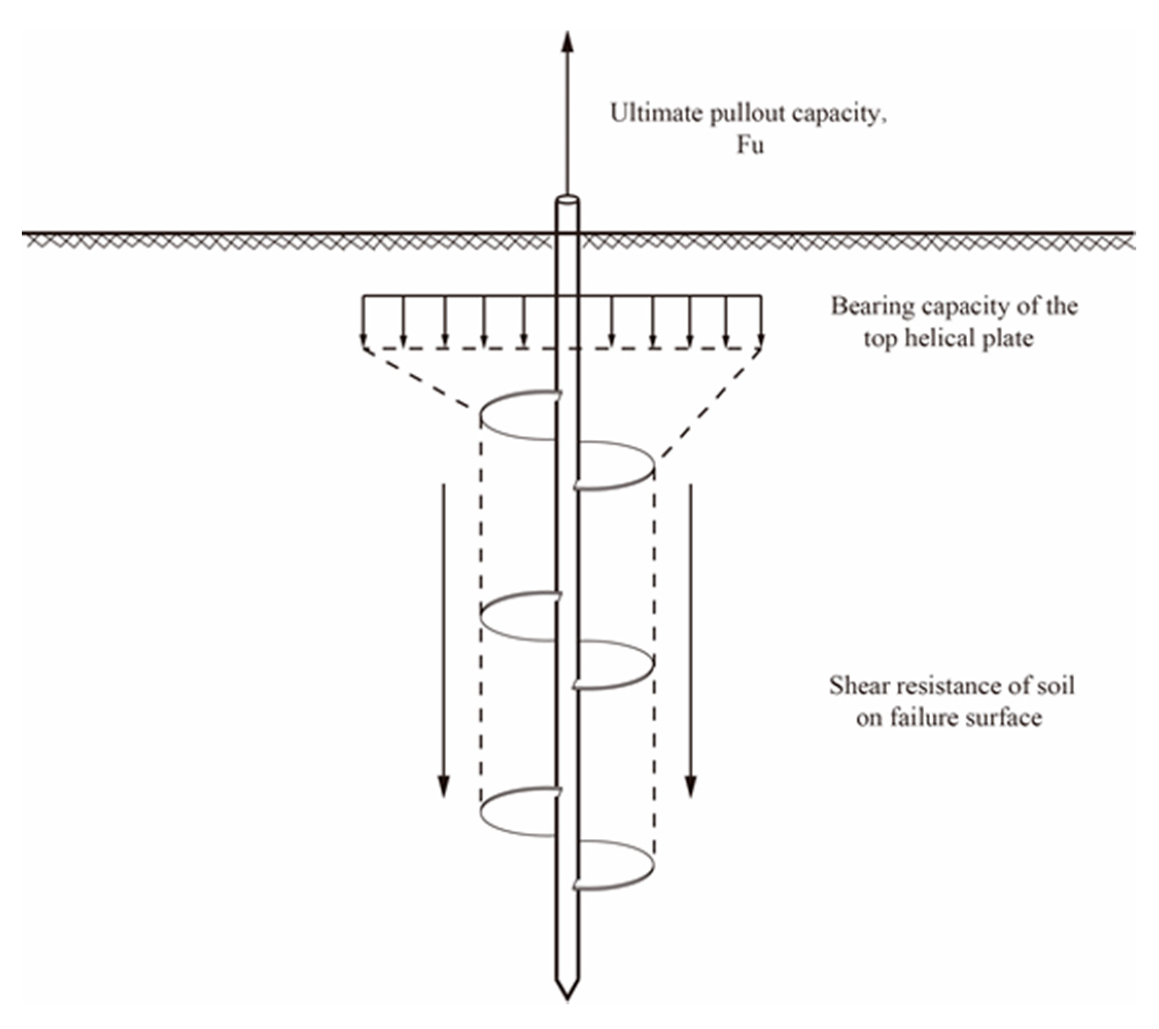
Helical anchors, as illustrated in Figure 1, are geotechnical foundation systems with helical bearing plates welded to a central steel shaft and can be applied to resist either compressive or tensile forces. Installation of the helical anchors is through applying a calculated torque to the top of the central steel shaft, which in turns transmit loads to helical plates. The major advantages of helical anchors include rapid and easy installation, minimal site disturbance, immediately load carrying capacity, direct verification of load capacity during installation, applicability to a wide range of soil types, etc. Although its early applications are limited mainly to the on-shore constructions notably in the industrial sectors, the helical anchor has proven its versatility in the past two decades by extending its use to offshore industry such as anchoring wind turbines and aquaculture equipment [1,2].
In the past research literature, a major focus on the pullout capacity of helical anchors in cohesive soils is the performance of helical anchors with different plate configurations [3,4,5,6,7], i.e., number of helical plates, n, the embedment depth of the uppermost helical plate, H, helical plate diameter, D, the ratio of helical plate spacing to diameter, S/D (See Figure 1). Based on previous research, helical anchors manufacturers propose two possible failure modes that depend on the relative spacing of helical plate [8]. Each failure mode corresponds to an empirical method to predict pullout capacity. Two empirical methods are the cylindrical shear method and the individual bearing method, respectively. Here, the former method is applicable for S/D ≤ 3, while the latter is used when S/D > 3. The specific calculation formula will be introduced in the next section.
Recently, the finite element method (FEM) was also extensively used to study the pullout behavior of helical anchors [9,10,11]. However, in practical engineering, owing to the tedious nature of the FEM, it is unrealistic to perform numerical simulation for every practice. Therefore, the accuracy of theoretical calculations is of utmost importance. Among various theoretical calculations of geotechnical engineering, there are assumptions about ideality and simplification of reality [12,13,14,15,16], which inevitably leads to model uncertainty. Therefore, many engineering technical design specifications and guidelines point out that there remains a need to evaluate the impact of model uncertainty [17,18,19]. The model uncertainty is usually characterized by a model factor, which is equal to the value of measured capacity divided by estimated solution [20,21,22]. The probabilistic distribution and statistical characteristics of the model factor can simply and completely represent the model uncertainty [23]. In previous studies, many efforts were expended to study the impact of model uncertainty on calculation theories and design guidelines [20,21,22]. Generally, there are two main points to be considered for characterizing the model factor: (1) verify the randomness; (2) determine its probability distribution and statistical characteristics. When a model factor is associated with input parameters, it should not be considered to be a random variable. Regression analysis can usually be used to remove the dependence on input parameters and the regression equation f is obtained. The use of regression equation f will greatly reduce the prediction error. As for the probability distribution and statistical characteristics, it can be determined by goodness-of-fit testing. Here, the framework to characterize the model uncertainty in Zhang et al. [20] is adopted in this work.
This paper presents the coupled Eulerian–Lagrangian (CEL) analyses to characterize the model uncertainty of using the cylindrical shear method (CSM) for estimating the vertical pullout capacity of helical anchors in cohesive soils. The principal objectives of this research are to (1) establish the regression equation for model uncertainty associated with the cylindrical shear method, an analytical method applicable to helical anchors failed in cylindrical shear mode (S/D ≤ 3); (2) develop a modified cylindrical shear method by incorporating the established regression equation into it so as to rectify its bias; (3) verify and characterize the randomness after the removal of bias. Please note that helical anchors failed in individual plate bearing failure mode (S/D > 3) are not within the scope of this study to limit the content to a manageable proportions.

2. The Cylindrical Shear Method

As explained above, the cylindrical shear method is applicable when the helical plates are sufficiently close to each other (S/D ≤ 3). As illustrated in Figure 2, it assumes a cylindrical-shaped failure mechanism between the helical plates [24]. The calculated pullout capacity of helical anchors is thus equal to the sum of shear resistance of the side face of the cylinder and the bearing resistance of the uppermost plate, as given by Equation (1a)
F u , c   =   π D S ( n 1 ) s u + 0.25 N c π D 2 s u
where n is number of helix plates, D helix plate diameter, S the spacing between helical plates, su the undrained shear strength. Nc is the breakout factor of the uppermost plate, which according to the design manual of Hubbell [8] can be estimated as
N c   =   1.2 H / D 9
where H denotes the embedment depth of the topmost helix plate.
Equation (1a) and Equation (1b) do not take into account the effect of soil weight on the pullout bearing capacity of helical anchors. If soil weight is considered, these equations can be re-expressed as:
F u , m = π D S ( n 1 ) s u + 0.25 N c π D 2 s u + 0.25 π D 2 ( n 1 ) S γ
with
N c = 1.2 H / D + γ H / s u 9
where γ denotes the unit soil weight. Note Equation (2a) is applicable only to predicting the capacity of the anchor when it is subject to perfectly vertical pull-out.

3. Load Test Databases

To characterize the model uncertainty, a load test database built by Tang and Phoon [22] was revisited. It includes 103 load tests of helical anchors with S/D ≤ 3, out of which 78 are small scale laboratory tests (see Table 1) and 25 are full-scale field tests (see Table 2). These laboratory tests are collated from two publications [3,4], where anchor of three different diameters (D = 0.033 m, 0.075 m, and 0.1 m) were tested under tension loading in soft to firm clays with the number of helical plates (n) varying between 2 and 5. The measured pullout capacity (Fu,m) span a fairly wide range (0.045 to 2.13 kN). The other 25 field tests were collected from three sources [5,6,7], where anchors of diameters ranging from 0.2 to 0.345m were loaded under tensile loading in clayey soil with shear strength su stretching from 31 to 99 kPa. Fu,m was reported to fall within a wide range 20 to 512 kN. As more detailed information regarding this database can be found in Tang and Phoon [22], they are not repeatedly described herein.

4. The Coupled Eulerian–Lagrangian Analyses

Three-dimensional large deformation finite element (LDFE) analyses were carried out using Abaqus 6.14. In the present work, the continuous pullout of a helical anchor under vertical load was studied using CEL finite element (FE) analyses, which was extensively employed to solve large deformation problems [25,26]. In the CEL analyses, the soil domain was modeled as Eulerian domain to cater the anticipative large deformation of soil elements, while helical anchors were modeled as Lagrangian body with infinite stiffness to improve computational efficiency. Additionally, a series of assumptions proposed by Wang et al. [10] were adopted as follows:
(1)
For simplicity, the actual shape of the helical plate was ignored, and the anchor plate was simplified to a regular circular plate with a thickness of 0.03D;
(2)
Helical anchors were assumed to be pre-embedded, namely the wished-in-place assumption was adopted.
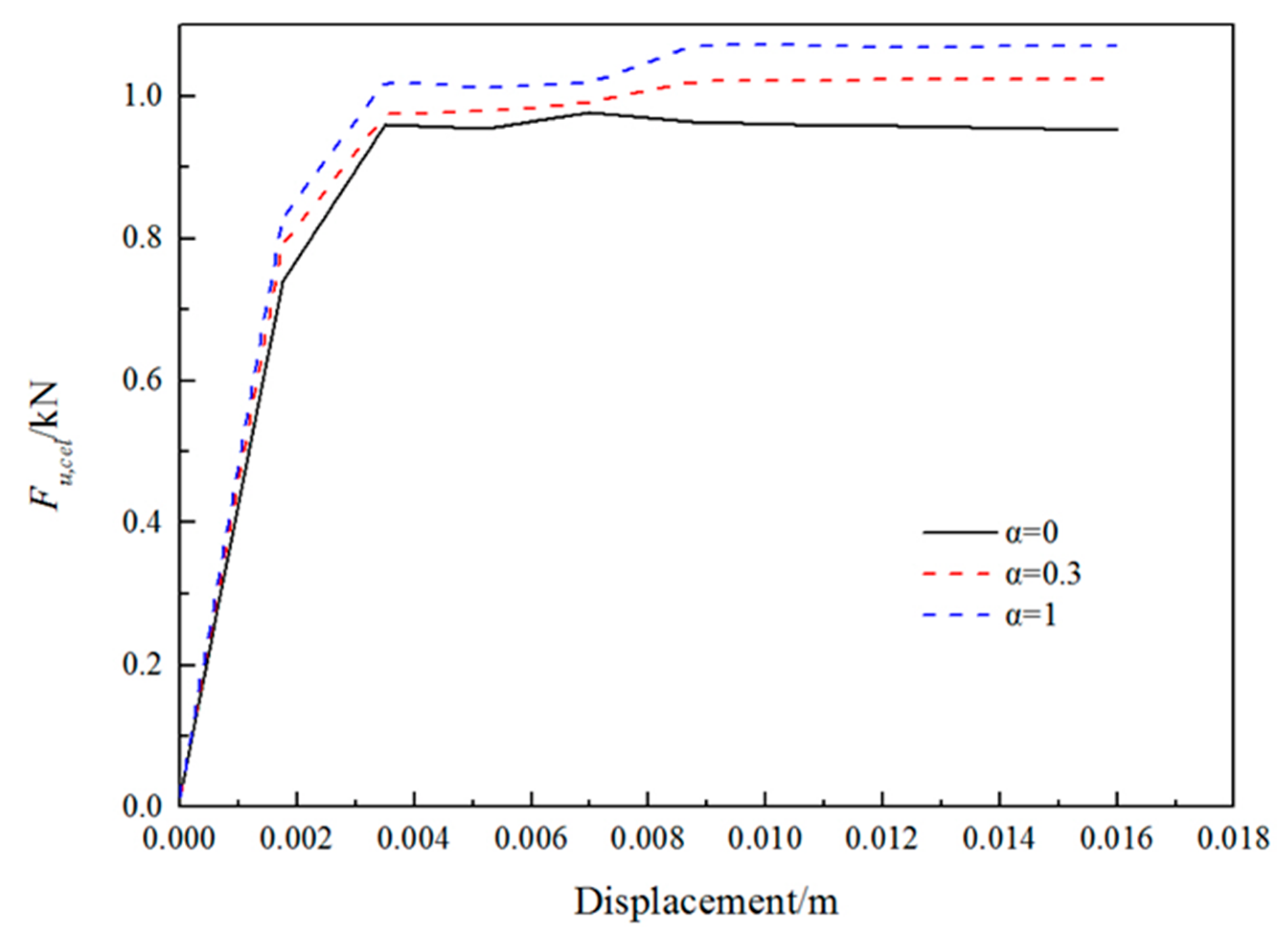
In all analyses, the interface between helical anchor and soil was commonly applied using a general contact form which can consider large sliding and separation between helical anchor and soil surfaces. The soil-anchor interface was assumed to be fully smooth for simplicity, such simplification is not expected to affect the analysis results significantly due to the slight discrepancy in pullout capacities between fully rough and smooth according to Merifield et al. [27] and Wang et al. [28]. To investigate the influence of different types of interfaces between soil and anchor on the pullout capacity of helical anchor, three different roughness conditions with interfacial frictional coefficient α = 0, 0.3, 1.0 were considered on soil-anchor interfaces, the results are shown in Figure 3. As shown in Figure 3, the peak pullout bearing capacity under the three different interface conditions are very close, and the error is within 7%. This clearly bore out the preceding notion that the interfacial roughness in the problem of helical anchor is not of much significance. In view of this, smooth interface was adopted mostly in the article to generate the main findings.
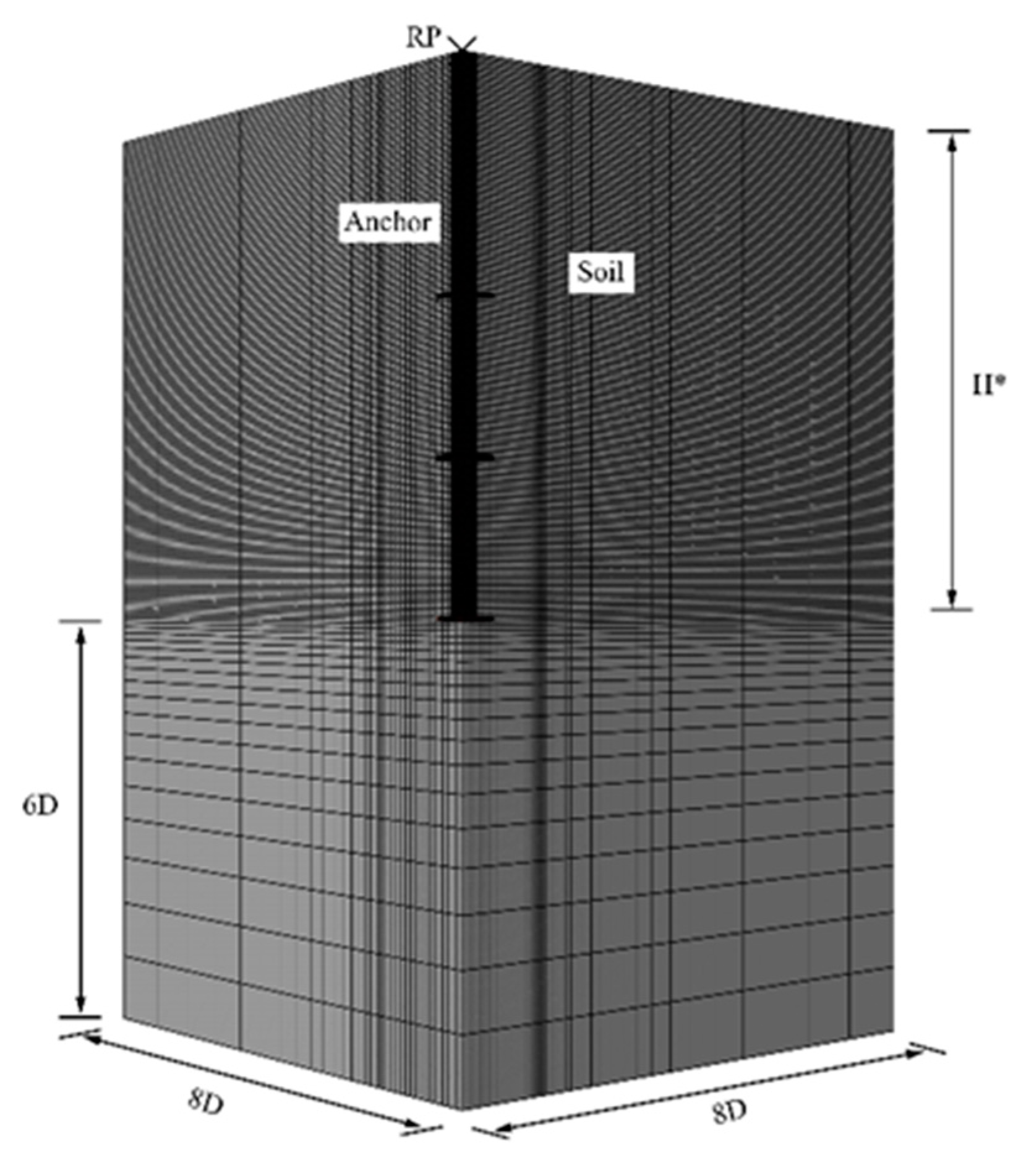
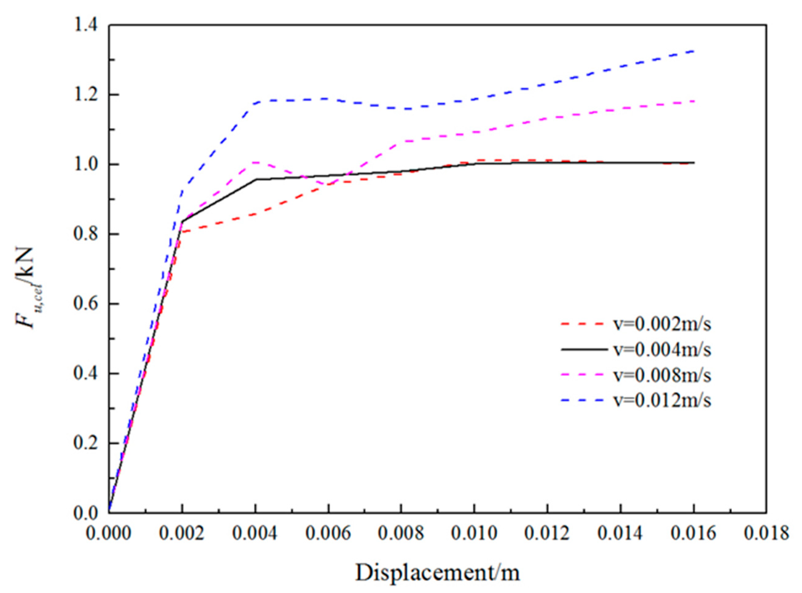
Figure 4 depicts the meshes and boundary conditions of the helical anchor and soil models adopted in the CEL analyses. Due to the simplification of the geometric shapes of helical anchors, the symmetry can be used in the FE analysis. Only a quarter model was employed to save computational time. The lateral boundaries were fixed at 8D away from the center, and the bottom boundary was set 6D below the lowermost helical plate, which was previously found to be large enough to minimize the boundary effect on the pullout capacity of helical anchors [11]. To balance the analysis efficiency and accuracy, as shown in Figure 4, the graded mesh was employed, the finer meshes were prescribed near the helical anchor, while coarser meshes were prescribed far away from the helical anchor towards the soil model boundaries. Velocity boundaries were adopted here, normal velocity on the lateral boundaries was limited, and vertical velocity was not permitted at the bottom of the base of the mesh. Generally, the failure of helical anchors can be determined by a developed slip surface [29]. The soil displacement occurs on this slip surface and the shear strength is completely mobilized. To model the pullout behavior, a displacement control method was employed, the reference point (RP) was set with a constant-displacement boundary condition in the vertical direction. The displacement of RP was set to 0.2D, which was sufficient to reach the maximum pullout capacity [10,11]. As for the pullout speed, a moderately high extraction rate (pullout speed) (v = 0.004 m/s) was adopted in this research. The load-displacement curves of anchor with different pullout speeds are shown in Figure 5. As can be noted from this graph, higher pullout rate generally entailed larger pullout loading, which reflect the kinetic effect. However, when the pullout speed became less than 0.004 m/s, the load-displacement curves roughly converged. Such a rate can thus balance computational efficiency and accuracy. It is for this reason, a v = 0.004 m/s was adopted in this research.
In this study, the cohesive soil was modeled as an elastic-perfectly plastic material obeying the Tresca yield criterion. The Poisson’s ratio was adopted as 0.49, which corresponded to an undrained state. Additionally, Wang et al. [10] pointed out that the pullout capacity of the helical anchor is largely independent of the Young’s modulus of the soil, so E = 500 su was taken as the representative value.

5. Model Factor for the Pullout Capacity of Helical Anchors

In the present work, the pullout capacity of a helical anchor is estimated via two methods, namely the CSM and the CEL analysis. As suggested by previous research, a model factor can be defined as the value of measured capacity divided by calculated solution
F u , m = M × F u , c a l
where Fu,m is the measured capacity, Fu,cal is the calculated solution, M is the model factor. It should be noted that different calculation methods correspond to their own specific model factors. In another word, a model factor calibrated from the CEL analysis cannot be applied to the CSM. When Fu,cal is calculated through CSM, denoted by Fu,csm, its corresponding model factor Mcsm is given by following equation
F u , m = M c s m × F u , c s m
When Fu,cal is calculated by CEL, labeled as Fu,cel, the model factor Mcel corresponds to Equation (3c)
F u , m = M c e l × F u , c e l
Generally, characterization of a model factor mainly contains two aspects: (1) verifying the randomness; (2) determining its probability distribution and statistical characteristics, such as the mean value and COV. Firstly, the verification of randomness can be achieved by calculating the Spearman correlation coefficient. Secondly, the distribution characteristics of the model factors can be determined by goodness-of-fit testing. It will be shown in the following part that Mcel can be considered to be a random variable, since it is independent of input parameters.
Osman and Bolton [30] compared the finite element method and calculation theory when studying the cantilever deflection in undrained clay, and defined the ratio of the two methods as the correction factor. Here, when comparing CEL and CSM, the correction coefficient η proposed by them is introduced.
F u , c e l = η × F u , c s m
The correction factor η is found to be influenced by the input parameters, so it is inappropriate to treat it as a random variable. Substituting Equation (4) into Equation (3c), we have
F u , m = M c e l × ( η × F u , c s m )
Combining Equations (5) and (3b), we can see that Mcsm is the product of η and Mcel:
M c s m = M c e l × η
Given that the correction coefficient η is related to the input parameters, the randomness of Mcsm is eliminated. As suggested by Kung et al. [31] and Zhang et al. [20], regression analysis based on FE numerical simulation is adopted here to eliminate the association of η with input parameters. In this work, the correction factor η is equal to the product of a systemic part f and a random residual part η* as follows
η = f × η *
By substituting Equation (7) into Equation (6), the Mcsm can be derived as
M c s m = M c e l × ( f × η * )
In the next few sections, the following steps are taken to quantify the model factor Mcsm:
(1)
On the basis of CEL analyses, numerical simulations are performed for the load tests in the database
(2)
Calculate the model factor Mcel of each CEL analysis, validate its randomness and determine its probability distribution and statistical characteristics
(3)
Generate a set of orthogonal experiments to perform regression analysis
(4)
Calculate the correction factor η of each orthogonal experiment
(5)
Determine systemic part f by using regression equations; verify the randomness of residual part η* and characterize its probability distribution
(6)
Substitute the regression equation f into the CSM to constitute the modified CSM (MCSM)
(7)
Collect another new load tests and verify the accuracy of MCSM

5.1. Comparison of CEL and Load Tests

Although the performance of the CEL analysis has been verified in previous research [11], the model uncertainty still exists due to the theoretical idealizations. For the given the anchor geometries and soil parameters in Table 1 and Table 2, Figure 6 plots the 103 pullout capacities calculated by performing CEL analysis and the 103 measured capacities. As depicted in Figure 6, the mean trend line of the ratio of CEL results to the measured pullout capacity is almost coincides with the 45° trend line, demonstrating that the CEL method is almost unbiased.
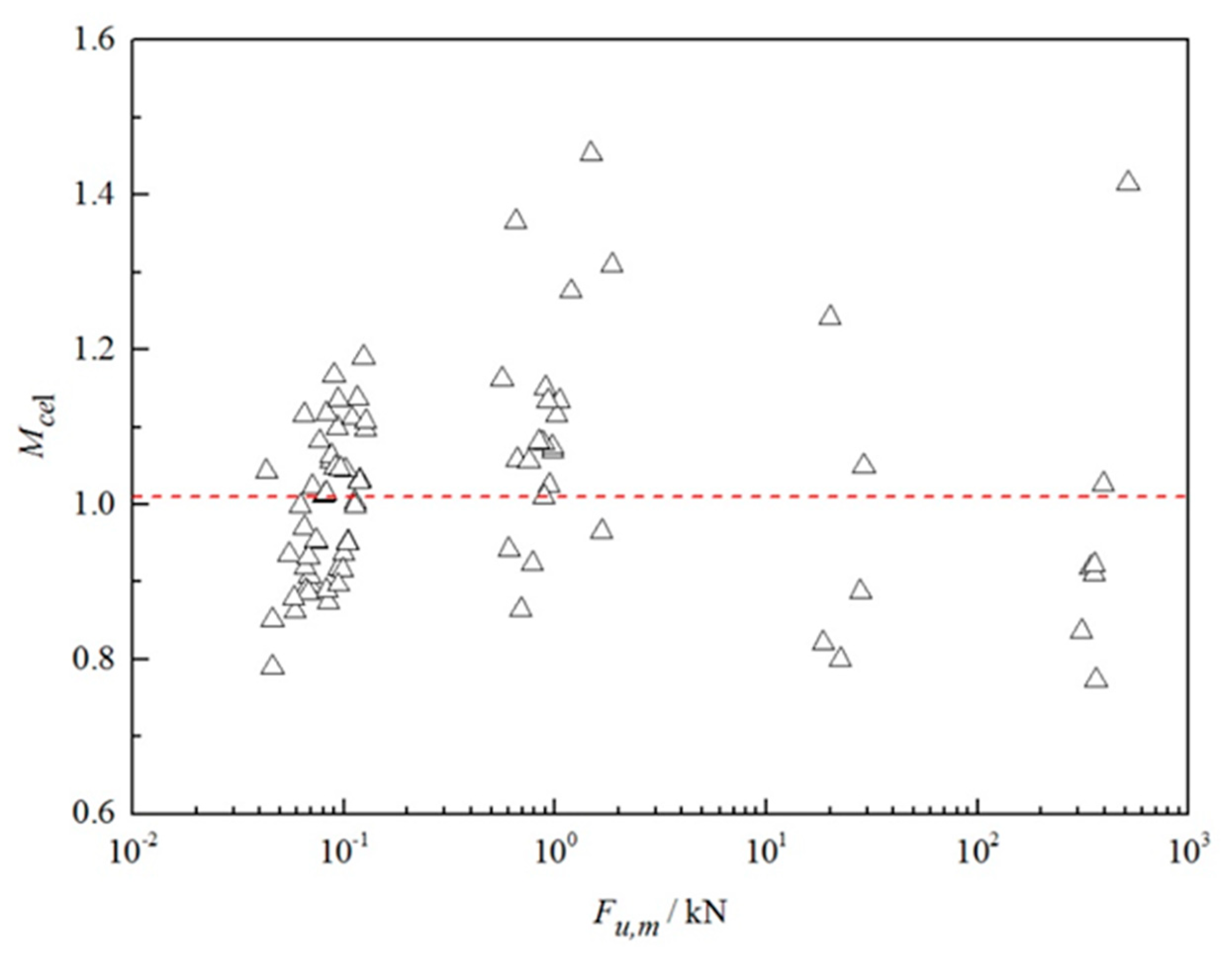
In the light of Equation (3c), the model factor Mcel is equal to the value of the measured capacities Fu,m divided by the capacities Fu,cel calculated from the CEL analysis. For the purpose of evaluating the model factor Mcel, the randomness of it should be first verified. Figure 7 displays the calculated Mcel of each case against the corresponding measured pullout capabilities. The model factor Mcel seems to be randomly distributed within the entire measured capacities range. To verify the randomness of Mcel, a Spearman rank correlation analysis is adopted in this study. Please note that a variable can be considered random when p-values of Spearman rank correlation are greater than 0.05. As illustrated in Table 3, all p-values are greater than 0.05. Consequently, the model factor Mcel can be considered random. In other words, the model factor Mcel is not a function of input parameters. Immediately following is to determine its probability distribution.
The frequency distribution histogram and the cumulative distribution function for Mcel are plotted in Figure 8a,b, respectively. The mean value and COV of Mcel are 1.02 and 0.1 respectively, demonstrating that the CEL analysis is almost unbiased. The p-value of K-S test shows that the lognormal distribution with a mean value of 1.02 and a COV of 0.1 is an appropriate probabilistic model for Mcel. Here, the model uncertainty of Mcel can be attributed to the following reasons:
(1)
The cohesive soil is modeled as elastic-perfectly plastic and the strain softening behavior of it is ignored
(2)
The actual shape of the helical anchor is simplified in the analysis and the pitch of it is neglected
(3)
The anchor-soil interface and contact conditions are assumed to be smooth
(4)
The above factors can unavoidably lead to some discrepancy between the estimated pullout capacities of the helical anchors by performing the CEL analysis and the measured pullout capacities, but in general, it is still an effective method to estimate the pullout capacities of helical anchors through the CEL analysis

5.2. Comparison of CSM and CEL

In this part, the model uncertainty of using CSM for estimating the vertical pullout capacity of helical anchors in cohesive soils will be characterized by the CEL analysis.
According to the previous studies, the pullout capacity of helical anchors is influenced by the following parameters: (1) helical plate diameter, D; (2) soil unit weight, γ; (3) undrained shear strength of soil, su; (4) embedment depth of uppermost helical plate, H; (5) helical plates spacing, S; (6) number of helical plates, n. The pullout capacity of helical anchor may be affected by many other factors, such as the soil disturbance effect and the strain softening behavior. Nevertheless, it is unrealistic to take all influencing factors into the evaluation of a model factor. Thus, the aforementioned six factors are incorporated and converted to four normalized parameters: γH/su, H/D, n and S/D. The value range of all parameters are given in Table 4. The realistic range of the four normalized parameters in this paper is as follows:
(1)
The number of helical plates n = 2, 3, 4, or 5
(2)
The dimensionless parameter γH/su = 0.4, 0.6, 0.8, 1.0, 1.2, 1.4, 1.6, 1.8, 2.0 or 2.2
(3)
The embedment ratio H/D = 1, 2, 3, 4, 5, 6, 7, 8, 9 or 10
(4)
The ratio of helical plate spacing to diameter S/D = 0.3, 0.6, 0.9, 1.2, 1.5, 1.8, 2.1, 2.4, 2.7, or 3.0
A total of 40 parameters sets are generated using orthogonal technique [32]. Every parameter set includes four normalized parameters in the aforementioned range. The comparison between CSM and CEL is implemented on the basis of the 40 cases.
Since Tang and Phoon [22] pointed out that the influence of unit weight of soil on the pullout capacity of helical anchors in cohesive soil is negligible, it is fixed at 16 kN⁄m3. Variance inflation factor (VIF) is a measure of the severity of complex collinearity in multiple linear regression models. The closer the VIF is to 1, the lighter the multicollinearity is, and the more orthogonal the input parameters are, and vice versa. If the VIF is greater than 10, the regression model has serious multicollinearity. In this paper, SPSS Statistics 25 is used to perform multicollinearity diagnosis for the 40 input parameters sets. The calculated VIF values of the four normalized parameters are listed in Table 4. As the table shows, all the values of VIF are almost close to 1, demonstrating that the four normalized parameters are orthogonal.

5.3. Correction Factor η

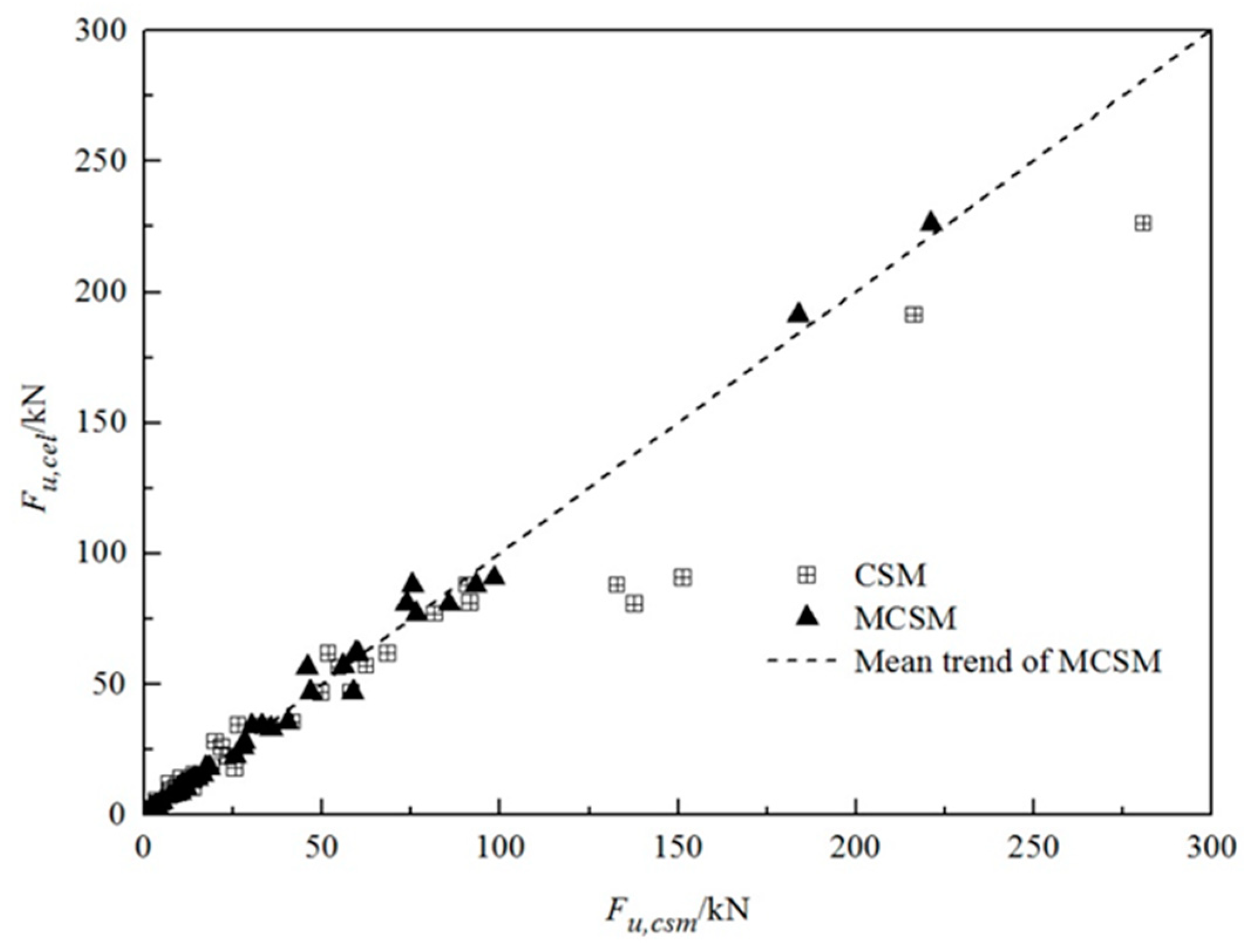
The pullout capacity of helical anchors in cohesive soil calculated by CSM (Fu,csm) and the calculated CEL results (Fu,cel) for these 40 cases are shown in Figure 9. After calculation, Fu,cel is on average 1.05 times Fu,csm. In other words, the mean value of correction coefficient η is equal to 1.05. However, it is incorrect to conclude that the CSM is in good agreement with the CEL analysis for the following two reasons. Firstly, η is influenced by the input parameter. The p-value associated with Spearman rank correlation is less than 0.05, which means this trend is statistically significant. Secondly, the COV of η is 0.266, which is high. Therefore, regression analysis is required to eliminate the correlation between the correction coefficient η and input parameters.

5.4. Regression Analysis

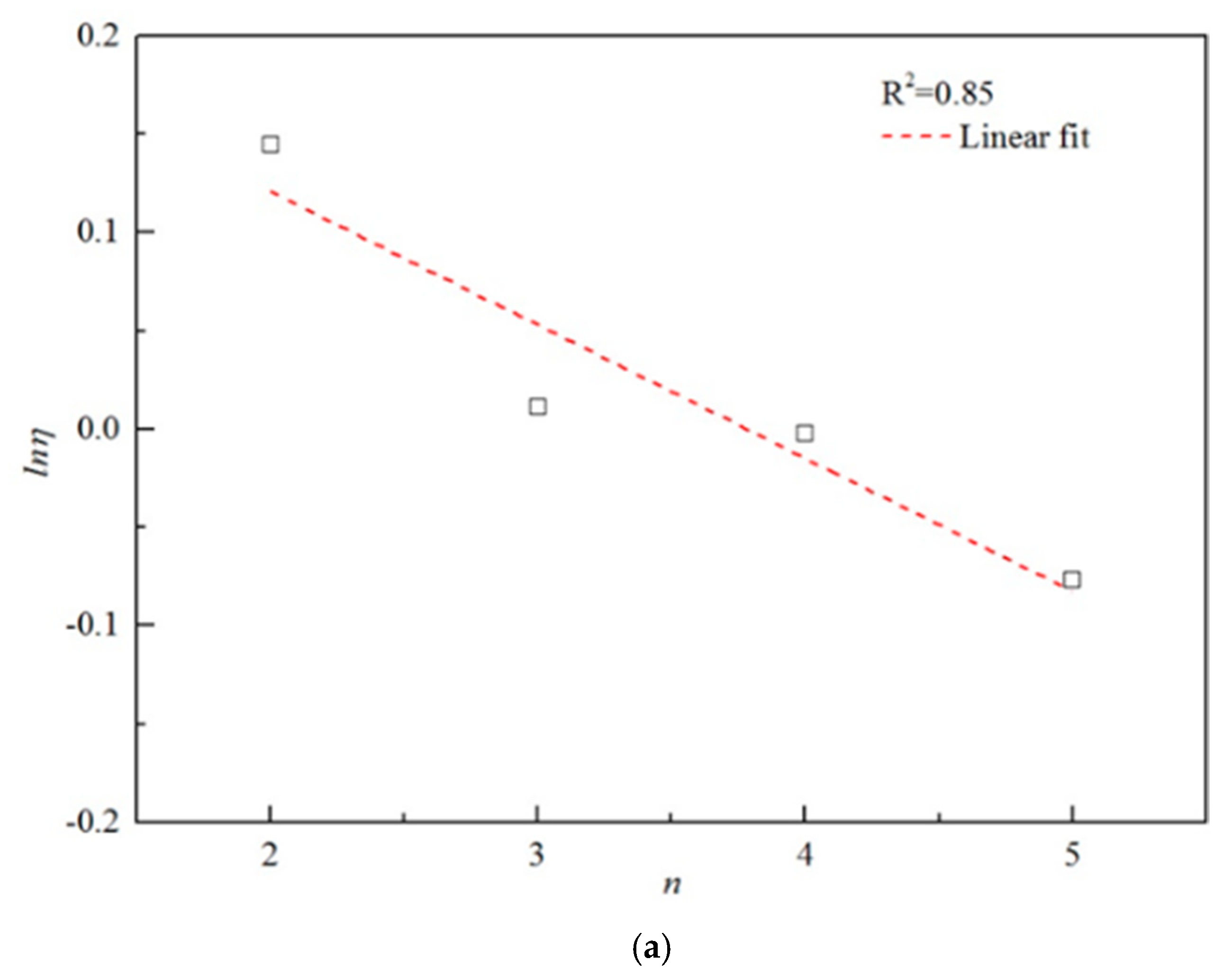
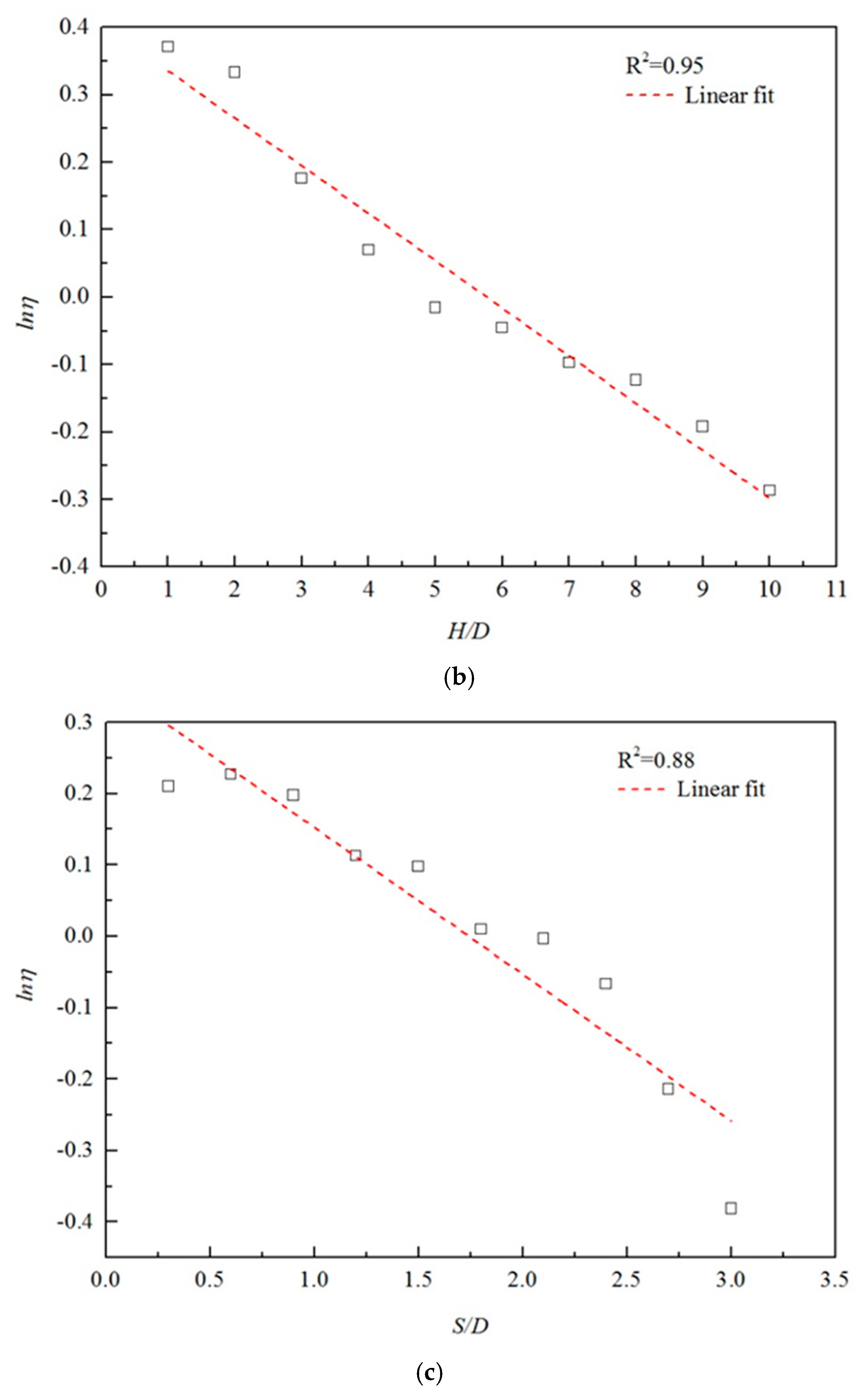
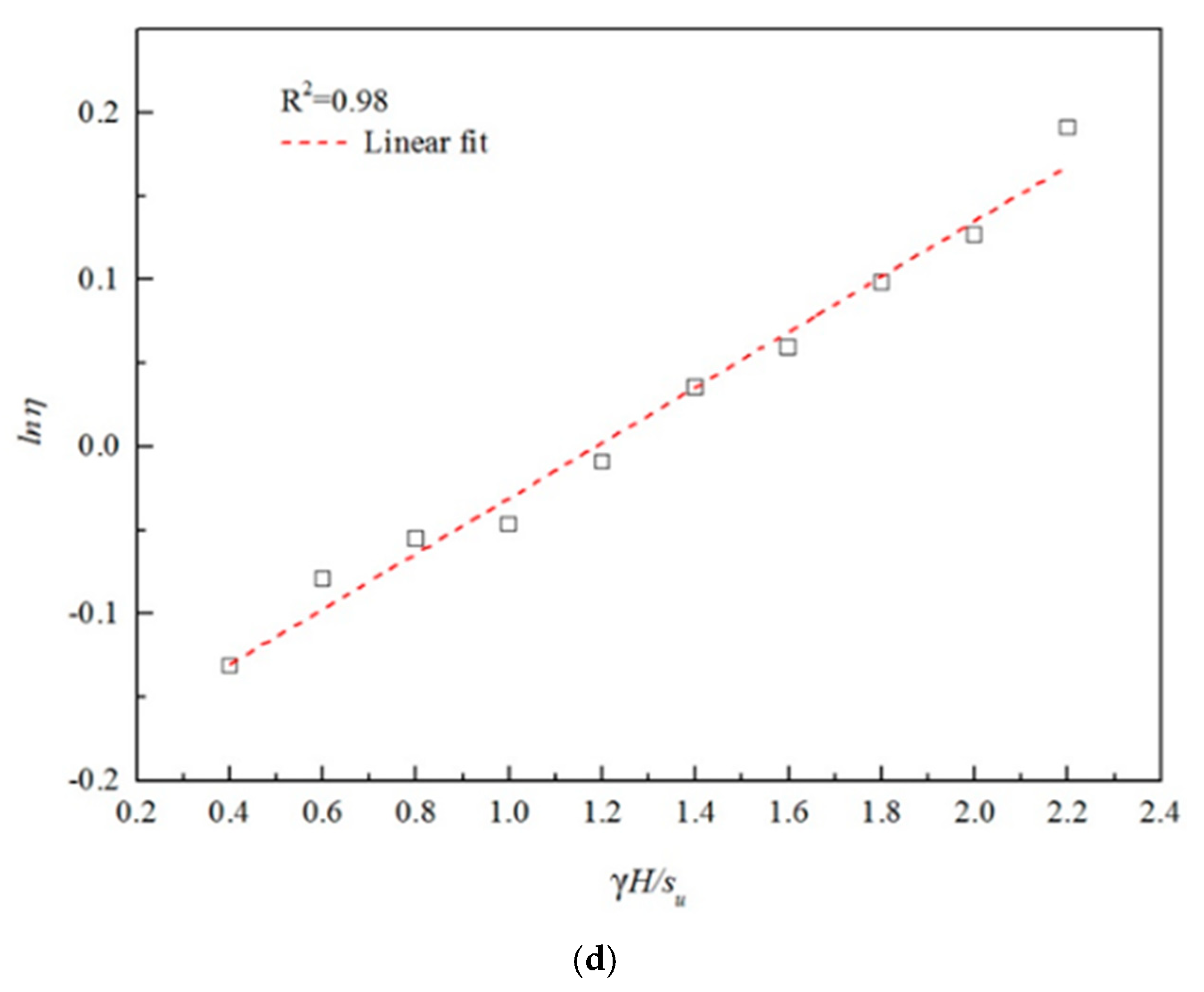
Figure 10a–d show the variation of the average value of lnη with each normalized parameter. The average value of lnη of each parameter at a certain level is the arithmetic average of all numerical simulations at that level. For instance, for parameter H/D, when the level is equal to 1, the mean value of lnη is the arithmetic mean value of four numerical simulations, and its input parameters are as follows:
(1)
H/D = 1, n = 2, S/D = 0.3, γH/su = 0.4
(2)
H/D = 1, n = 3, S/D = 0.9, γH/su = 1.2
(3)
H/D = 1, n = 4, S/D = 1.2, γH/su = 1.2
(4)
H/D = 1, n = 5, S/D = 1.0, γH/su = 2.0
Please note that H/D is fixed at 1 in these CEL analyses. Due to the orthogonality of these simulations, average η value associated with H/D = 1 is independent on the other three parameters. As can be seen from Figure 10a–d, lnη varies linearly with γH/su, H/D, n and S/D, and its coefficient of determination (R2) is greater than 0.8. Hence, lnη can be fitted as a linear function of the previously described four normalized parameters.
According to the trend as exhibited in Figure 10a–d, a multiplicative model f can be proposed to account for the systematic variation η of with the normalized parameters as follows:
f = e b 0 e b 1 n e b 2 S / D e b 3 H / D e b 4 γ H / s u
where {bi }(i = 0, ⋯, 4) are the model coefficients. Substituting Equation (9) into Equation (7), the η can be obtained
η = e b 0 e b 1 n e b 2 S / D e b 3 H / D e b 4 γ H / s u × η *
ln η = b 0 + b 1 n + b 2 S / D + b 3 H / D + b 4 γ H / s u + ln η *
where η* is the random residual part of η that shows no dependency on the four normalized input parameters. Therefore, η* can be considered to be a random variable. When the natural logarithm of both sides of Equation (10a) is taken at the same time, it can be found that both sides of the equation show a linear relationship, as shown in Equation (10b), and then the model coefficient can be obtained. In addition, then SPSS Statistics 25 is used in this work for performing multiple linear regression analyses. Each obtained model coefficient is listed in Table 5. The value of R2 of the regression equation f is 0.863, which is close to 1, indicating that the regression line fits the observed value well. It should be noted that the proposed regression equation f does not take into account the interaction effect of four normalized parameters. Thus, the proposed regression equation f is only applicable the parameters given in Table 4. In this paper, H/D ranges from 1 to 10. Therefore, when regression equation f is used, those field test where H/D is out of range will use Equation (2b) to correct the value of H/D.
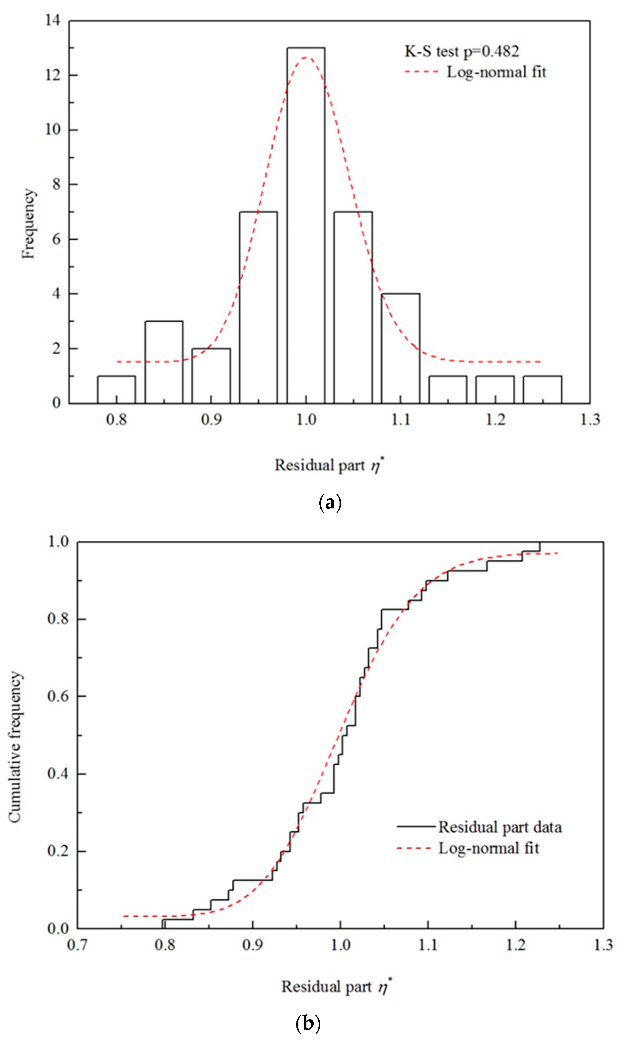
To verify the randomness of the residual part η*, Spearman rank correlation analysis is performed. Based on the regression equation f, the systematic part is removed and the residual part η* of 40 numerical simulations is obtained. As can be seen from Table 3, all the p-values for η* are all more than 0.05. Unlike dependence of η on input parameters, the residual part η* is not associated with input parameters. It means that η* is a random variable. After checking the randomness of η*, immediately following is to determine the probability distribution of it. Figure 11a,b plot the frequency distribution histogram and the cumulative distribution function of η* for 40 numerical simulations. The mean value of η* is equal to 1.0, and the COV of it is 0.09. Herein, COV of η* is much smaller than η. In addition, the p-value of K-S test demonstrates that the lognormal probability model is a reasonable probabilistic model for η*.
The original CSM multiplied with the regression equation f constitutes the MCSM, the F′u,csm denotes the pullout capacity calculated from MCSM, then the correction factor for the F′u,csm is equal to the residual part η*, the equation is as follows:
F u , c s m = f × F u , c s m
F u , c e l = η * × F u , c s m
Figure 9 plots F′u,csm obtained from Equation (11a) against the CEL results Fu,cel for these 40 simulations. The discrepancy between F′u,csm and Fu,cel is relatively small, which demonstrates that the performance of MCSM is better than CSM. Meanwhile, the correction factor for the MCSM is equal to the residual part η* which shows no dependence on the input parameters.

5.5. Comparison of CSM and Load Tests

5.5.1. Probability Model for the Modified Model Factor Mcsm

According to Equation (8), the model factor Mcsm is the product of the model factor Mcel, the regression equation f and the residual random part η*. After using the CSM to predict the pullout capacity of the aforementioned 103 tests and calculating the corresponding model factors Mcsm, the Spearman rank correlation analysis of model factors Mcsm is carried out. The results indicate that Mcsm cannot be directly considered to be a random variable due to its association with the input parameters. As described earlier, the original CSM multiplied with the regression equation f constitutes the MCSM. Then the model factor for MCSM( M′csm) is equal to the measured pullout capacity divided by the calculated capacity of MCSM and is also the product of the CEL model factor Mcel and the residual part η*, the equations are as follows:
F u , m = M c s m × F u , c s m
M c s m = M c e l × η *
As mentioned earlier, both the CEL model factor Mcel and the residual part η*, follow a lognormal distribution, and M′csm is the product of these two variables. It is well known that the product of two statistically independent lognormal random variables also follow a lognormal random distribution. Based on previous results, the mean value and COV of Mcel are 1.02 and 0.1, while the corresponding values for η*, are 1.0 and 0.09.
M e a n = E M c s m = E M c e l η * = e E ln M c e l + E ln η * + 0.5 ( σ ln M c e l 2 + σ ln η * 2 ) .  
V a r i a n c e = σ M c s m 2 = σ M c e l η * 2 = e 2 ( E ln M c e l + E ln η * ) [ e 2 ( σ ln M c e l 2 + σ ln η * 2 ) e ( σ ln M c e l 2 + σ ln η * 2 ) ]
where E ln ( · ) and σ ln ( · ) is given by
σ ln x 2 = ln ( 1 + σ x 2 / E x 2 ) ,   E ln x = ln E x 0.5 σ ln x 2
Using Equation (5) and the corresponding mathematical operation rules Equation (13a–c) as documented in Phoon and Tang [21], the calculated mean value of M′csm is 1.02, with a COV of 0.13. By comparison, it can be found that the MCSM is more accurate than the original CSM.

5.5.2. Validation of Model Factor M′csm

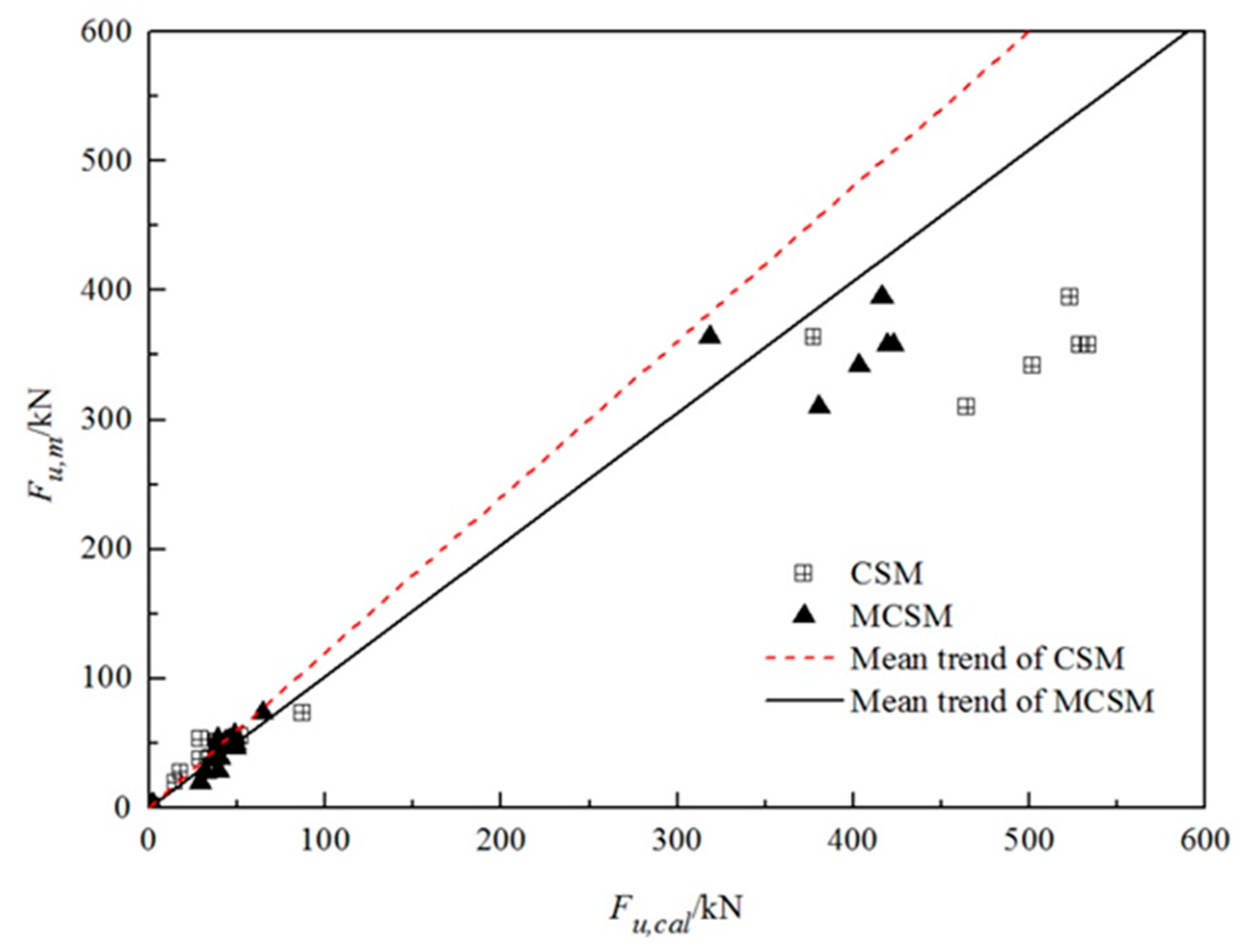
The load test databases adopted for calibration of Mcel consist of 78 laboratory tests and 25 field tests, which are large enough to be divided into two databases. In this work, a calibration database consists of 50 load tests, while the validation database consists of 53 load tests. The pullout capacity calculated from the CSM and the measured capacity in shown Figure 12. The mean value and COV of the model factor Mcsm for original CSM is 1.2 and 0.18 respectively. In addition, the p-values for Spearman rank correlation indicate that Mcsm cannot be regarded as a random variable directly. From Figure 12, it can be seen that most Fu,csm are smaller than the measured capacity Fu,m.
The application of regression equation f removes systemic dependence on input parameters. The original CSM multiplied with the regression equation f constitutes the MCSM. Figure 12 also plots the MCSM (solid triangle) results calculated from Equation (11a) against the measured results. As the figure shows, the mean trend line for F′u,csm is almost coincides with the 45° trend line. In addition, the mean value of M′csm is 1.02, which is equal to the mean value calculated by Equation (13a). This indicates that the accuracy of the MCSM has been improved when compared with the original CSM. The COV of MCSM is 0.13, which is less than the large COV of 0.18 associated with the original CSM. Similarly, the COV value of MCSM is consistent with the theoretically value calculated from Equation (13b). The next step is to carry out the Spearman rank correlation analysis.
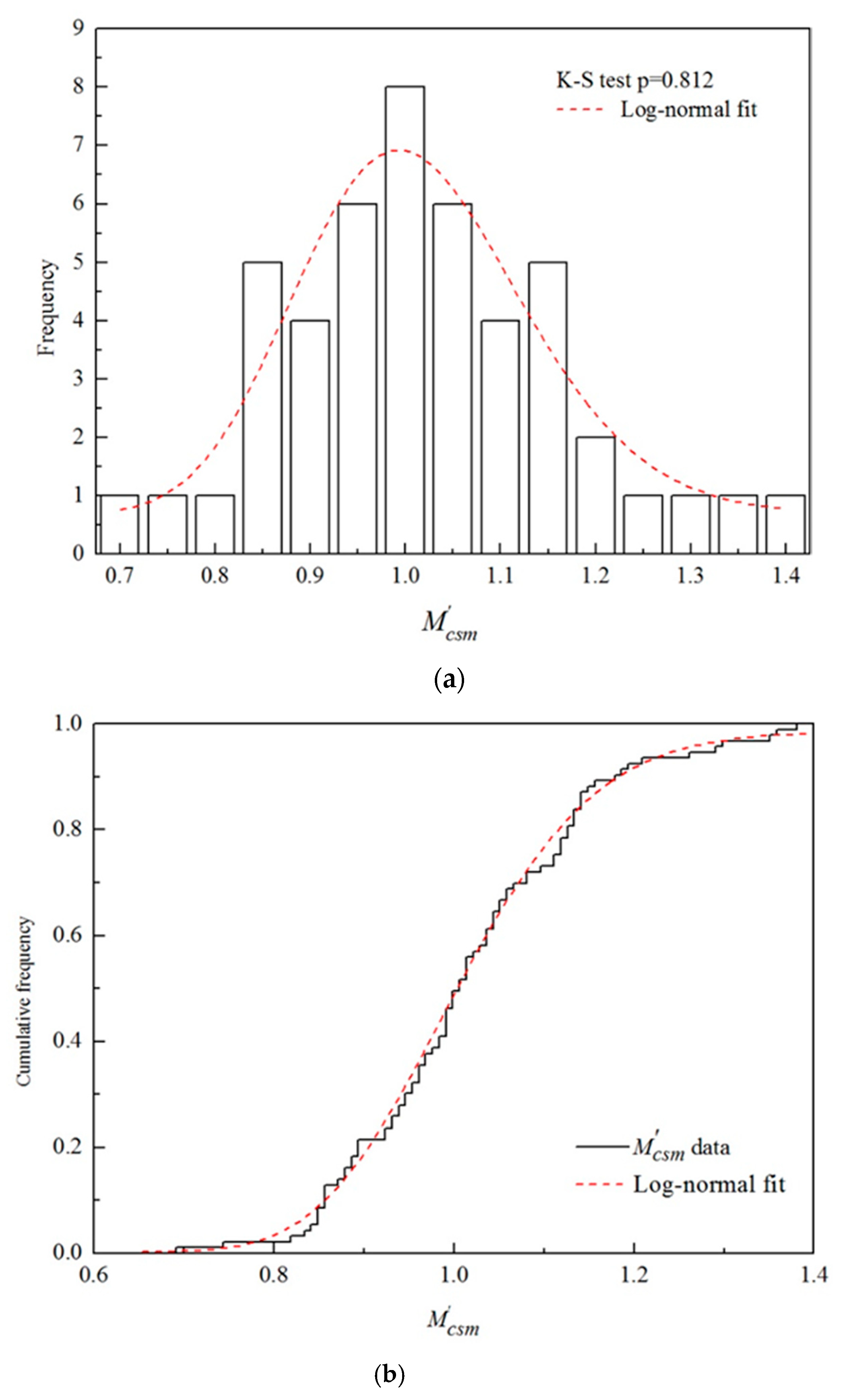
All the p-values of the Spearman rank correlation analysis for M′csm are shown in Table 3, which are all greater than 0.05. It implies that M′csm is not influenced by input parameters, and it could be considered to be a random variable. Then probability distribution of M′csm is verified. Figure 13a,b plot the frequency distribution histogram and the cumulative distribution function of M′csm. In addition, the p-value of K-S test demonstrates that the lognormal probability model with a mean value of 1.02 and a COV of 0.13 is an appropriate probabilistic model for M′csm.

6. Comparison of Prediction Accuracy of MCSM, MCSM in Tang and Phoon [22], and Original CSM

In this section, the prediction accuracy of MCSM, MCSM in Tang and Phoon [22], and original CSM is examined by compared to field tests collected from the previous literature.

6.1. Load Test Database for Comparing Prediction Accuracy

Tappenden et al. [33] conducted five static axial load tests on helical anchors installed in stiff silty clay and hard clay till. These anchors were installed in Alberta and British Columbia. The undrained shear strength su was 75 kPa and 145 kPa respectively. The diameter of plate was 0.356 m and 0.762 m respectively. Number of helical plates varied from 1 to 3. The relative spacing of helical plate (S/D) was 1.5 or 3. The embedment depth of the anchor ranged from 3 m to 6 m.
Sakr [34] performed one full-scale load test in soft to firm clay. The investigation site was located in northern Manitoba, Canada. The undrained shear strength of the soil at the investigation site was 24 kPa. The anchor configurations used for test consisted of three helical plates with the same diameter of 0.711 m, and the diameter of the anchor shaft is 0.219 m. The embedment depth of the anchor was 7.9 m, with a S/D = 2.5.
In the work by Sakr [35], four full-scale tension (pullout) testing programs were presented. The soil at the investigation site was very stiff to very hard clay till soils, with the su ranging from 83 kPa to 225 kPa. Number of helical plates were 1,2,2,3 respectively. The embedment depth of the anchor varied from 5.6 m to 18.5 m. Helical plates for these anchors were spaced at either 2 or 3 times their diameter.
Harnish and El Naggar [36] conducted three pullout load tests in Lamont near Edmonton, Alberta. The investigation site consisted of glacial till, and the undrained shear strength su was equal to 244 kPa. The anchor used for test were composed of 1 or 2 helical plates. All of these anchors were installed at a depth of 6.86 m. For the anchor with two helical plates, the S/D value was 3.
In total, 13 filed load tests are collected to compare the prediction accuracy of pullout capacity. The specific information of these tests is summarized in Table 6.

6.2. Results of Accuracy Comparison

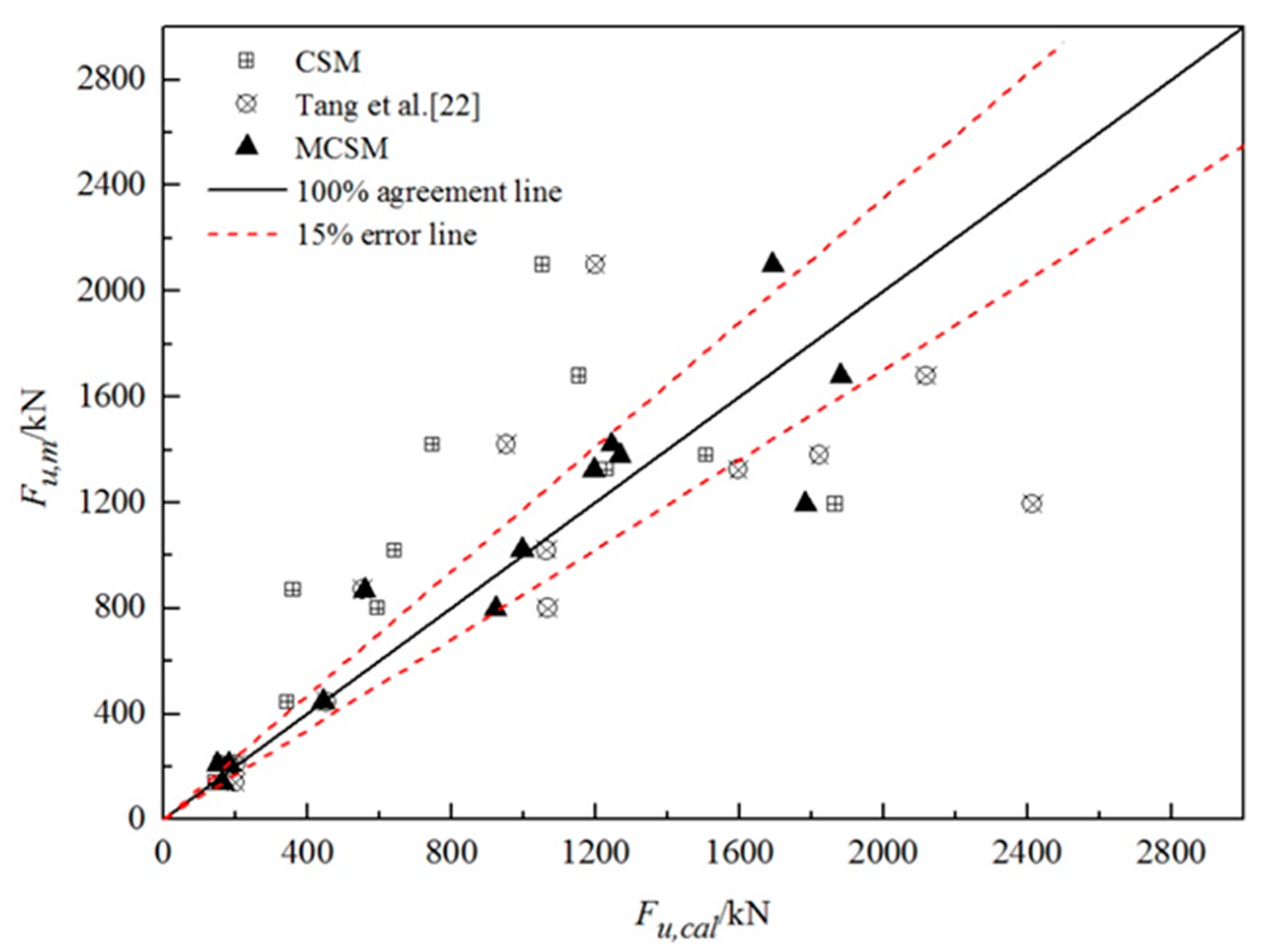
The pullout capacities calculated from the MSCM, MCSM in Tang and Phoon [22], original CSM are compared with the measured pullout capacities. The results of the comparison are summarized in Table 7 and plotted in Figure 14. It can be seen from the chart that the error range of capacity predicted by MCSM is mostly within 15%. By contrast, when the regression equation proposed by Tang and Phoon [22] is used to calculate the pullout capacity, the error range is mostly above 20%. Meanwhile, when original CSM is used, the maximum difference remains at 25% or above. This indicates that when predicting the pullout capacity of helical anchors in cohesive soil, the use of MCSM can provide a relatively more accurate prediction result.

7. Summary and Conclusions

This study conducts the coupled Eulerian−Lagrangian finite element analyses to characterize the model uncertainty of using cylindrical shear method to predict the pullout capacity of helical anchors in cohesive soils. The model factor in this paper is equal to the value of measured capacity divided by estimated solution. After conducting CEL analysis on 78 laboratory tests and 25 field tests, it is found that the CEL analysis is a reasonable tool to predict the pullout capacities of helical anchors, and model factor Mcel can be considered to be a random variable with a lognormal distribution, and its mean value and COV are 1.02 and 0.1, respectively. The correction coefficient η is introduced when comparing CSM and CEL. η is found to be associated with four normalized parameters: γH/su, H/D, n and S/D. Then η is divided into a systemic part f and a random residual part η*. To determine the systemic part f, 40 sets of orthogonal experiments are generated for regression analysis. The regression equation f could be used to remove systematic variation. The residual part η* could be considered to be a random variable with a lognormal distribution, and its mean value and COV are 1.0 and 0.09, respectively.
The original CSM multiplied with the regression equation f constitutes the MCSM. By computation and analysis, model factor M′csm should be a random variable that follows a lognormal distribution. To validate this, 103 load tests are divided into two groups, a calibration database consists of 50 load tests, while the validation database consists of 53 load tests. By calculating and verifying the mean and COV of model factor M′csm of tests in the validation database, it is found to be consistent with the results calculated by the previous formula. The lognormal probability model with a mean value of 1.02 and a COV of 0.13 is an appropriate probabilistic model for M′csm.
Finally, 13 field tests are collected to compare the accuracy of predicting the pullout capacity of helical anchors using original CSM, MCSM in Tang and Phoon [22] and MCSM. The results show that the prediction accuracy of MCSM is more accurate than the other two methods, and the error range mostly within 15%, which might be helpful for engineers to estimate the pullout capacity of helical anchors in cohesive soils more confidently.
It should be acknowledged that owing to the complexity of the problem, several assumptions or simplifications have been adopted, as explained earlier. As such, the present research outcomes are inevitably subject to a few limitations. Firstly, the strain softening behavior of soil has been disregarded, which may somewhat overestimate the pull−out bearing capacity of the helical anchor. Secondly, the shape of the helical anchor has been simplified. To remedy these limitations, more works are planned in future studies.

Author Contributions

Conceptualization, Methodology, Writing, Verification and Software: P.C.; Writing, Investigation, Verification and Software: J.T.Y.; Verification and Software: F.L., J.J.D. All authors have read and agreed to the published version of the manuscript.

Funding

This research was funded by the graduate scientific research and innovation foundation of Chongqing, China (Grant/Award Numbers: CYS18023), the National Natural Science Foundation of China (No. 51778091).

Conflicts of Interest

The authors declare no conflict of interest to the work submitted.

References

  1. Byrne, B.W.; Houlsby, G.T. Helical piles: An innovative foundation design option for offshore wind turbines. Philos. Trans. R. Soc. A 2015, 373, 20140081. [Google Scholar] [CrossRef] [PubMed] [Green Version]
  2. Cortes-Garcia, L.D.; Landon, M.E.; Gallant, A.P.; Huguenard, K.D. Assessment of Helical Anchor Capacity in Marine Clays for Aquaculture Applications. In Proceedings of the Geo-Congress 2019, Reston, VA, USA, 24–27 March 2019; pp. 299–307. [Google Scholar]
  3. Rao, S.N.; Prasad, Y.V.S.N.; Shetty, M.D. The behaviour of model screw piles in cohesive soils. Soils Found. 1991, 31, 35–50. [Google Scholar] [CrossRef] [Green Version]
  4. Rao, S.N.; Prasad, Y.V.S.N.; Veeresh, C. Behaviour of embedded model screw anchors in soft clays. Geotechnique 1993, 43, 605–614. [Google Scholar] [CrossRef]
  5. Mooney, J.S.; Adamczak, S.; Clemence, S.P. Uplift capacity of helix anchors in clay and silt. In Proceedings of the Uplift Behavior of Anchor Foundations in Soil, Detroit, MI, USA, 24 October 1985; pp. 48–72. [Google Scholar]
  6. Stuedlein, A.W.; Holtz, R.D. Bearing Capacity of Spread Footings on Aggregate Pier Reinforced Clay. J. Geotech. Geo Environ. Eng. 2013, 139, 49–58. [Google Scholar] [CrossRef]
  7. Lutenegger, A.J. Cylindrical Shear or Plate Bearing—Uplift Behavior of Multi-Helix Screw Anchors in Clay. In Proceedings of the International Foundation Congress & Equipment Expo, Orlando, FL, USA, 15–19 March 2009; pp. 456–463. [Google Scholar]
  8. Hubbell, Inc. Chance® Technical Design Manual-Edition 3. A. B. Chance Div., Hubbel, Inc. 2014. Available online: http://www.ebsgeo.com/ModuleFile/getFile_Chance%20%C2%AE%20Technical%20Design%20Manual%20-%20Edition%203?id=2181 (accessed on 21 September 2020).
  9. Merifield, R.S. Ultimate uplift capacity of multiplate helical type anchors in clay. J. Geotech. Geo Environ. Eng. 2011, 137, 704–716. [Google Scholar] [CrossRef]
  10. Wang, D.; Merifield, R.S.; Gaudin, C. Uplift behaviour of helical anchors in clay. Can. Geotech. J. 2013, 50, 575–584. [Google Scholar] [CrossRef]
  11. Kwon, O.; Lee, J.; Kim, G.; Kim, I.; Lee, J. Investigation of pullout load capacity for helical anchors subjected to inclined loading conditions using coupled Eulerian-Lagrangian analyses. Comput. Geotech. 2019, 111, 66–75. [Google Scholar] [CrossRef]
  12. Phoon, K.K.; Kulhawy, F.H. Characterization of geotechnical variability. Can. Geotech. J. 1999, 36, 612–624. [Google Scholar] [CrossRef]
  13. Dithinde, M.; Phoon, K.K.; Ching, J.; Zhang, L.; Retief, J.V. Statistical characterization of model uncertainty. Reliab. Geotech. Struct. ISO2394 2016, 5, 127–158. [Google Scholar] [CrossRef]
  14. Yi, J.T.; Huang, L.Y.; Li, D.Q.; Li, Y. A large-deformation random finite-element study: Failure mechanism and bearing capacity of spudcan in a spatially varying clayey seabed. Geotechnique 2019, 70, 392–405. [Google Scholar] [CrossRef]
  15. Yi, J.T.; Pan, Y.T.; Huang, L.Y.; Xu, S.J.; Liu, Y.; Phoon, K.K. Determination of limiting cavity depths for offshore spudcan foundations in a spatially varying seabed. Mar. Struct. 2020. [Google Scholar] [CrossRef]
  16. Peng, Y.; Ding, X.; Xiao, Y.; Deng, X.; Deng, W. Detailed amount of particle breakage in nonuniformly graded sands under one-dimensional compression. Can. Geotech. J. 2020, 57, 1239–1246. [Google Scholar] [CrossRef]
  17. Joint Committee on Structural Safety. Probabilistic Model Code; Joint Committee on Structural Safety, 2006. Available online: https://www.jcss-lc.org (accessed on 21 September 2020).
  18. Lesny, K.; Akbas, S.O.; Bogusz, W.; Burlon, S.; Vessia, G.; Phoon, K.K.; Tang, C.; Zhang, L. Evaluation and consideration of model uncertainties in reliability based design. In Joint ISSMGE TC 205/TC 304 Working Group on “Discussion of Statistical/Reliability Methods for Eurocodes, 20-64; International Society for Soil Mechanics and Geotechnical Engineering: London, UK, 2017; Available online: http://www.icsmge2017.org/download/19th%20ICSMGE_Workshop_TC205&304.pdf (accessed on 21 September 2020).
  19. DNV. Recommended Practice: Statistical Representationof Soil Data. DNVGL-RP-C207; Det Norske Veritas (DNV): Oslo, Norway, 2017. [Google Scholar]
  20. Zhang, D.M.; Phoon, K.K.; Huang, H.W.; Hu, Q.F. Characterization of Model Uncertainty for Cantilever Deflections in Undrained Clay. J. Geotech. Geo Environ. Eng. 2015, 141, 04014088. [Google Scholar] [CrossRef] [Green Version]
  21. Phoon, K.K.; Tang, C. Model Uncertainty for the Capacity of Strip Footings under Positive Combined Loading. In Geotechnical Safety and Reliability; ASCE: Denver, CO, USA, 4–7 June 2017; pp. 40–60. [Google Scholar] [CrossRef]
  22. Tang, C.; Phoon, K.K. Model uncertainty of cylindrical shear method for calculating the uplift capacity of helical anchors in clay. Eng. Geol. 2016, 207, 14–23. [Google Scholar] [CrossRef]
  23. Phoon, K.K.; Tang, C. Characterisation of geotechnical model uncertainty. Georisk Assess. Manag. Risk Eng. Syst. Geohazards 2019, 13, 101–130. [Google Scholar] [CrossRef]
  24. Kulhawy, F.H. Uplift behavior of shallow soil anchors-an overview. In Uplift Behavior of Anchor Foundation in Soil; ASCE: New York, NY, USA, 1985; pp. 1–25. [Google Scholar]
  25. Qiu, G.; Henke, S.; Grabe, J. Application of a Coupled Eulerian–Lagrangian approach on geomechanical problems involving large deformations. Comput. Geotech. 2011, 38, 30–39. [Google Scholar] [CrossRef]
  26. Liu, F.; Yi, J.; Cheng, P.; Yao, K. Numerical simulation of set-up around shaft of XCC pile in clay. Geomech. Eng. 2020, 21, 489–501. [Google Scholar] [CrossRef]
  27. Merifield, R.S.; Lyamin, A.V.; Sloan, S.W.; Yu, H.S. Three-Dimensional Lower Bound Solutions for Stability of Plate Anchors in Clay. J. Geotech. Geo Environ. Eng. 2003, 129, 243–253. [Google Scholar] [CrossRef] [Green Version]
  28. Wang, D.; Hu, Y.; Randolph, M. Three-dimensional large deformation finite-element analysis of plate anchors in uniform clay. J. Geotech. Geo Environ. Eng. 2010, 136, 355–365. [Google Scholar] [CrossRef]
  29. Lee, J.; Kwon, O.; Kim, I.; Kim, G.; Lee, J. Cyclic pullout behavior of helical anchors for offshore floating structures under inclined loading condition. Appl. Ocean Res. 2019, 92, 101937. [Google Scholar] [CrossRef]
  30. Osman, A.S.; Bolton, M.D. A new design method for retaining walls in clay. Can. Geotech. J. 2004, 41, 451–466. [Google Scholar] [CrossRef]
  31. Kung, G.T.; Juang, C.H.; Hsiao, E.C.L.; Hashash, Y.M.A. Simplified Model for Wall Deflection and Ground-Surface Settlement Caused by Braced Excavation in Clays. J. Geotech. Geo Environ. Eng. 2007, 133, 731–747. [Google Scholar] [CrossRef]
  32. Tan, O.; Zaimoglu, A.S.; Hinislioglu, S.; Altun, S. Taguchi approach for optimization of the bleeding on cement-based grouts. Tunn. Undergr. Space Technol. 2005, 20, 167–173. [Google Scholar] [CrossRef]
  33. Tappenden, K.M.; Sego, D.C. Predicting the Axial Capacity of Screw Piles Installed in Canadian Soils. In Proceedings of the Canadian Geotechnical Conference, Ottawa, ON, Canada, 21–25 October 2007; pp. 1608–1615. [Google Scholar]
  34. Sakr, M. Helical Piles for Power Transmission Lines: Case Study in Northern Manitoba Canada; Almita Manufacturing Ltd.: Ponoka, AB, Canada, 2008. [Google Scholar]
  35. Sakr, M. Installation and Performance Characteristics of High Capacity Helical Piles in Cohesive Soils. DFI J. J. Deep Found. Inst. 2012. [Google Scholar] [CrossRef]
  36. Harnish, J.; Naggar, M.H.E. Large-diameter helical pile capacity—Torque correlations. Can. Geotech. J. 2017, 54, 968–986. [Google Scholar] [CrossRef] [Green Version]
Figure 1. Schematic diagram of a helical anchor.
Jmse 08 00738 g001
Figure 2. Cylinder-shaped failure mechanism of helical anchor (modified from Rao et al. [3]).
Jmse 08 00738 g002
Figure 3. The pullout capacity under the three different interface conditions.
Jmse 08 00738 g003
Figure 4. Mesh and applied boundary condition of FE analysis (represents an example only).
Jmse 08 00738 g004
Figure 5. Load displacements curves of anchors pulled out at different rates.
Jmse 08 00738 g005
Figure 6. Measured capacity versus the CEL calculated capacity.
Jmse 08 00738 g006
Figure 7. Distribution of Mcel in the range of measured capacity.
Jmse 08 00738 g007
Figure 8. (a) Frequency distribution histogram of Mcel; (b) Cumulative distribution function of Mcel.
Jmse 08 00738 g008
Figure 9. Calculated capacity from CSM and MCSM versus the CEL calculated capacity.
Jmse 08 00738 g009
Figure 10. Variation trend of lnη with four normalized parameters: (a) n; (b) H/D; (c) S/D; (d) γH/su.
Jmse 08 00738 g010aJmse 08 00738 g010bJmse 08 00738 g010c
Figure 11. (a) Frequency distribution histogram of η*; (b) Cumulative distribution function of η*.
Jmse 08 00738 g011
Figure 12. Calculated capacity from CSM and MCSM versus the measured capacity.
Jmse 08 00738 g012
Figure 13. (a) Frequency distribution histogram of M′csm; (b) Cumulative distribution function of M′csm.
Jmse 08 00738 g013
Figure 14. Comparison of prediction accuracy of three methods.
Jmse 08 00738 g014
Table 1. 78 small scale laboratory tests in the database (data from Tang and Phoon [22]).
ReferencesSerial NumbernD/(m)H/DS/Dsu/(kPa)Fu,m/(kN)
Rao et al. [3]130.0756.13213.51.86
230.11.531.537.10.73
320.12.292.297.10.97
420.0756.131.676.20.65
540.0756.131.336.20.9
630.11.531.537.11.34
720.151.531.537.11.67
820.12.292.297.10.63
930.11.531.537.10.97
1030.151.021.027.11.72
1130.0756.1326.20.83
1230.0756.130.8313.51.48
1340.0756.131.3313.52.13
1420.0756.131.6713.51.19
1520.12.292.297.10.91
1630.0756.130.836.20.71
Rao et al. [4]1740.03361.54.40.113
1830.0331.51.530.046
1950.03381.130.087
2050.03341.130.074
2140.07551.37.70.973
2250.033101.130.093
2330.075827.71.02
2450.03311.14.40.084
2520.0332.32.330.043
2630.03382.330.083
2730.0751.31.37.70.605
2830.03342.330.071
2950.03361.14.40.113
3040.033101.54.40.127
3140.07511.37.70.691
3240.03321.54.40.094
3330.033102.34.40.124
3440.03331.54.40.1
3530.03312.330.055
3630.03362.34.40.11
3730.03322.330.062
3840.07521.37.70.784
3940.07581.37.71.05
4030.075427.70.884
4130.075327.70.839
4250.03331.130.069
4340.03331.530.069
4440.03381.54.40.119
4520.0332.32.34.40.065
4640.03321.530.066
4750.03321.130.066
4850.033101.14.40.127
4940.0331.11.14.40.068
5040.03311.54.40.083
5140.03361.530.08
5240.03381.530.087
5330.075127.70.662
5430.033102.330.09
5550.03381.14.40.118
5630.03332.330.065
5750.03361.130.081
5830.03382.34.40.116
5950.03311.130.059
6030.03322.34.40.091
6130.03362.330.077
6250.03341.14.40.104
6340.03311.530.058
6430.03312.34.40.082
6530.075227.70.755
6640.07541.37.70.94
6730.0331.51.54.40.068
6850.03331.14.40.099
6950.03321.14.40.094
7030.075527.70.922
7140.07531.37.70.889
7240.033101.530.094
7340.03341.54.40.104
7430.03342.34.40.102
7530.03332.34.40.096
7640.03341.530.074
7720.075227.70.562
7840.0331.11.130.046
Table 2. 25 full-scale field tests in the database (data from Tang and Phoon [22]).
ReferencesSerial NumbernD/(m)H/DS/Dsu/(kPa)Fu,m/(kN)
Mooney et al. [5]7930.24840.924853.2
8030.24840.924853.2
8130.24880.924849.4
8230.24880.924851.7
8330.248100.924849.5
8430.248100.924847.2
8530.248120.924849.6
8630.248120.924846.9
Stuedlein [6]8750.34519393342
8850.34519399358
8940.3319397364
9050.34519398358
9150.34519397395
9250.34519386310
9340.3319385516
Lutenegger [7]9430.2280.753120
9530.22333129
9630.2271.133127.9
9730.2261.53118.6
9830.2252.253122.4
9930.2130.756137.9
10030.2121.136138.9
10130.2111.56151.1
10230.2102.256155.7
10340.2836173.5
Table 3. The p-value of variables for Spearman rank correlation analysis.
Variables
Parameters
γ H/DnS/D
M c e l 0.7830.5990.1060.303
η * 0.7110.8100.7660.823
M c s m 0.5160.4890.1110.280
Table 4. Realistic range of four normalized parameters.
ParametersRange of ValuesVIF
γ H/su0.4–2.21.01
H/D1–101.11
n2–51.08
S/D0.3–3.01.04
Table 5. Model coefficient of the regression equation.
CoefficientsValues
b 0 0.823
b 1 −0.068
b 2 −0.172
b 3 −0.056
b 4 0.161
Table 6. 13 field tests for comparing prediction accuracy.
ReferencesTest NumbernD/(m)Embedment Depth/(m)S/Dsu/(kPa)Fu,m/(kN)
Tappenden [33]T110.7625.9 145800
T220.3565375210
T320.762631451325
T430.35651.575210
T530.35631.575140
Sakr [34]T630.7117.9324445
Sakr [35]T710.9145.6 2251680
T820.7625.932251195
T920.81314.32831420
T1020.81318.52117.52100
Harnish and El Naggar [36]T1110.4576.86 244870
T1210.6106.86 2441020
T1320.6106.8632441380
Table 7. Results of prediction accuracy comparison of pullout capacity.
Test Number F u , m / ( kN ) F u , c s m / ( kN ) Relative Error
of CSM(%)
Tang’s Method Predicted Capacity/(kN)Relative Error
of Tang’s Method(%)
F u , m c s m / ( kN ) Relative Error
of MCSM(%)
T1800595.13−25.611067.6533.46923.4315.43
T2210158.69−24.44185.63−11.60150.49−28.34
T313251229.51−7.211596.1220.461195.90−9.74
T4210158.69−24.44201.09−4.24181.98−13.34
T5140143.582.55199.7142.65163.7917.00
T6445343.59−22.79453.171.84443.65−0.30
T716801155.21−31.242118.3926.091881.9512.02
T811951866.4056.182414.19102.021783.4549.24
T91420748.10−47.32952.18−32.951245.36−12.30
T1021001052.57−49.881200.09−42.851692.07−19.43
T11870360.21−58.60553.75−36.35559.35−35.71
T121020641.77−37.081063.754.29996.58−2.30
T1313801507.109.211822.3232.051269.02−8.04