Abstract
Estimating ship resistance accurately in different water depths is crucial to design a resistance-optimized hull form and to estimate the minimum required power. This paper presents a validation of a new procedure used for resistance correction of different water depths proposed by Raven, and it presents the numerical simulations of a Kriso container ship (KCS) for different water depth/draught ratios. Model-scale and full-scale ship resistances were predicted using in-house computational fluid dynamics (CFD) code: HUST-Ship. Firstly, the mathematical model is established and the numerical uncertainties are analyzed to ensure the reliability of the subsequent calculations. Secondly, resistances of different water depth/draught ratios are calculated for a KCS scaled model and a full-scale KCS. The simulation results show a similar trend for the change of model-scale and full-scale resistance in different water depths. Finally, the correction procedure proposed by Raven is briefly introduced, and the CFD resistance simulation results of different water depth/draught ratios are compared with the results estimated using the Raven method. Generally, the reliability of the HUST-Ship solver used for predicting ship resistance is proved, and the practicability of the Raven method is discussed.
1. Introduction
The shallow-water effect refers to the situation that the hydrodynamic performance of a ship clearly changes when the water depth is less than a certain critical value. For a channel that produces the shallow water effect, we divide it into two categories: (1) one is the channel that only considers the limited water depth and its effect on the hydrodynamic performance of the ship, which is called the shallow water channel; and (2) the other is the channel in which both the water depth and the width are limited, causing an effect on the hydrodynamic performance of the ship, which is called the restricted channel. The hydrodynamic characteristics of ships in navigation will change and differ significantly when encountering restricted channels versus shallow water channels. Generally, the effects of shallow water can be summarized into the following three aspects: (1) the change of attitude manifested as the change of trim and sinkage; (2) the increase of ship resistance; and (3) worse maneuverability of the ship. For some high-speed vessels, the water depth needs to be rather deep to avoid the influence of shallow water, which cannot always be guaranteed. Especially in recent years, the shallow-water effect of vessels becomes more and more evident with the increase in tonnage of ships. The obvious sinkage of vessels in shallow water is caused by many bottom touching accidents, which makes it difficult for the safe navigation of vessels encountering shallow-water channels. In addition, the obvious increase of ship resistance in shallow water leads to a worse speed–power characteristic, which directly affects the operational efficiency of the vessel. An accurate prediction of ship resistance in shallow or confined water is crucial. Model tests are the most common way to predict the resistance of a ship, and the resistance of the full-scale ship can be obtained utilizing extrapolation. Even though much practice has proved the reliability of the extrapolation approach, the Reynolds number similarity between the ship model and the full-scale ship cannot be achieved, which results in significant differences between the model-scale and full-scale ship flow. The ITTC-57 correlation line [1] used to build a relationship between the resistance of a scaled model and the full-scale ship may not be accurate in shallow water. Zeng et al. [2] mentioned in their paper “This is probably due to the backflow and/or a different wetted surface”. Raven [3] also suggested considering the scale effect in the extrapolation. The rapid development of computational performance and numerical methods promotes the development of computational fluid dynamics (CFD) [4], and the Unsteady Reynolds Average Navier-Stokes equation (URANS) CFD solver is becoming another practical tool used for predicting the hydrodynamic characteristics of ships. In addition to saving time and money, another advantage of using a CFD solver is that it is easier to obtain the local flow characteristics. URANS simulations were conducted for a KCS [5]; the effective power and the increase of resistance in a series of designed head waves are predicted. In addition, the effect of speed loss on the reduction of effective power is explained. Yang et al. [6] presented a study on the air cavity under a stepped planing hull based on the finite volume method (FVM), and a mesh convergence study was conducted to ensure the accuracy of the simulation. Cucinotta et al. [7,8] analyzed the performance of a multi stepped air cavity planing hull using URANS CFD code. Duy et al. [9] investigated the stern flow field for several transom configurations of a KCS using a viscous CFD solver. Jachowski et al. [10] predicted the squat of a KCS scaled model in shallow water using the CFD method; the results show quite good agreement with the empirical method of Hooft [11]. Numerical prediction of the resistance of a barge ship with different calculation velocities at different water depth-to-ship draft ratios (T/H) was conducted [12]. It can be seen in the study that the increase of resistance becomes increasingly obvious with the decrease of water depth and the increase of velocity, which means that the increase of resistance is related to both velocity and water depth. JI et al. [13] conducted a 3D numerical simulation to research the relationship of the sediment movement induced by the compounding effects of ship-generated waves, water flow due to ship propellers, and the influence of ship and channel characteristics. Linde et al. [14] proposed a 3D hydrodynamic numerical model to predict ship resistance and sinkage of an inland ship in restricted waterways; the results showed that the ship resistance is more sensitive to water depth than channel width. Du et al. [15] studied inland vessels in the fully-confined waterway, and the characteristics of resistance and waves were analyzed. CFD simulations of the pure sway tests in a shallow water towing tank were conducted for the DTC container ship model using URANS solver [16]. From the study, the ability of URANS CFD solver to simulate the pure sway tests in a shallow water towing tank was proved by comparing with the test data. Researchers also conducted the maneuvering tests of a scaled ship model with different water depths and speeds [17], the results show that the shallow water effect has an adverse effect on ship maneuverability, which is manifested by the increase of turning diameter and the decrease of course stability. Simulations of straightforward, turning and zig-zag motions for a cargo ship were carried out [18]; as the depth–draft ratio decreases, the ship’s resistance increases and the maneuverability becomes worse.
Furthermore, some researchers proposed methods for resistance correction in different water depths. The earliest method that can be found for correcting shallow water resistance was proposed by Schlichting [19]. A further method of Lackenby [20] was proposed by the reanalysis of Schlichting’s method, which was recommended by the International Towing Tank Conference in 2014 [21]. Methods proposed at that time was based on less experimental data due to limited resources. In recent years, with the development of numerical methods and experimental technology, researchers derived some new methods based on numerical calculations and experimental data. Jiang introduced a mean effective speed, which can be calculated by the mean sinkage, ship speed, and water depth [22]. In his study, Jiang found that the model resistance is almost a unit function of the effective speed and independent of the water depth. Raven [23] proposed a new method to correct the resistance in shallow water after theoretical analysis and numerical calculations, which was recommended by the ITTC in 2017 [24].
For the great importance of estimating ship resistance in different water depths, it is significant to predict the hydrodynamic characteristics of a ship in different water depths. The existing relevant literature mainly focuses on the very shallow water; most of their water depths/draft ratios are less than 2. However, the limited water depths of a larger value play a very important role in reality. This paper studied the influence of water depth on ship resistance; several large limited water depths were chosen to conduct the towed resistance simulations for a Kriso container ship (KCS). Resistance and attitude in different water depths for the scaled model and the full-scale KCS were calculated. Before performing the calculation at different water depths, analysis of numerical uncertainties was carried out. For model scale, the sensitivity of grid spacing from the bottom of the ship to the tank bottom was also studied. Numerical tanks with large width were established to ignore the influence of limited width. The chosen water depths were slightly larger to match the constraints of Raven’s method. The in-house CFD solver HUST-Ship was employed to carry out the calculations. The simulation results were compared with the predicted results of Raven’s model.
2. Mathematical Model
2.1. Governing Equations and Turbulence Model
The in-house CFD code HUST-Ship, based on the finite difference method (FDM), is employed to solve the unsteady incompressible RANS equations coupled with the continuity equation:
where is the Reynolds stress with turbulent pulsation; is the fluctuating velocity, is the dynamic pressure coefficient, is Reynolds stress tensor, and is the Reynolds number.
The Froude number and Reynolds number are defined as:
where is the fluid viscosity coefficient, g is the acceleration of gravity, and and are the ship service speed and the length between perpendiculars, respectively.
The turbulent equation uses an SST (shear–stress transport) equation turbulence model to close the governing equation. The equations for turbulent flow energy k and turbulent dissipation rate ω are:
where and are the diffusion ratios of k and ω, respectively; and are the turbulent diffusion terms for k and ω, respectively; is the turbulent kinetic energy generated by the average velocity gradient; is the production term of the ω equation; and and are the custom source terms for the k and ω equations respectively.
2.2. Coordinate System and 6-DOF Equations
In the process of the towing simulation, the attitude (pitch and heave) of a KCS always changes with the pressure distribution on the hull surface, hence the need for the 6-DOF equations [25]. The equations involve a time item; therefore, the unsteady RANS equation was solved with the 6-DOF system integrated into the solution program. Figure 1 shows the coordinate system of the HUST-Ship program. The 6-DOF equations can be written as:
in which, , and are the components of moment of inertia with respect to the gravity center; X, Y, Z and K, M, and N are the components of external forces and moments acting on the hull, respectively. The ship position is described in an earth fixed coordinate system with X pointing south, Y pointing east, and Z pointing upward. The origin of the ship local coordinate system is set at the intersection of the design waterline and the bow. The velocities for 6-DOF motions (u, v, w, p, q, r) are reported in a ship local coordinate system with the x-axis positive toward stern, the y-axis positive toward starboard and the z-axis positive upward. The 6-DOF motions of the ship are reported at the center of gravity.
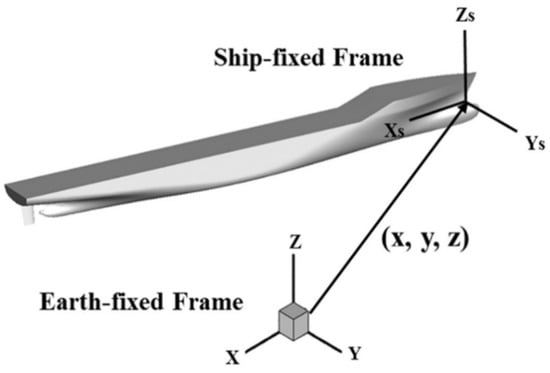
Figure 1.
The coordinate system of HUST-Ship.
To obtain the trim angle and sinkage of a KCS, only 2-DOF motion related to pitching and heaving are solved in this paper.
2.3. Level-Set Method
HUST-Ship can capture the change of free surface based on the single-phase level-set [26] method. The level-set method is a general calculation method for tracking interface motion, which was widely used in the field of numerical simulation; the free surface was thought of as an interface. The term φ is the distance from a point of the field to the free surface. It is always the case that φ = 0 represents all points on the position of the free surface, a positive value of φ represents a particle in air and a negative value represents a point in water. Compared with the classical multi-phase level-set method and the volume of fluid (VOF) method [27], the discrepancy of single-phase level-set method is very small as it ignores the effects of air since the influence of air on free-surface ships is very small. The level-set function [28] is:
where is the vector of the velocity within the domain and only the flow of water would be solved in the area of . The position of the free surface (φ = 0) can be obtained using interpolation. The boundary condition for the velocity at the interface can be defined as:
in which is the normal vector and can be defined as:
The main advantage of the level-set method is that the quality of the grid is stable and easy to control.
2.4. Wall Function
For the calculations of full-scale vessels, the high Reynolds number led to a need for a smaller boundary layer thickness, which increased the grid quantity. Therefore, a wall function is introduced to deal with the near-wall situation, and a multi-layer wall function of a two-point model is adopted, wherein the velocity of the first node far away from the wall can be obtained from the following equation:
where is the tangential velocity; is the wall shear stress; and is the dimensionless wall distance. The constant values are κ = 0.41 and B = 5.1; ΔB is a correction term considering wall friction and thinning of the logarithmic layer, which is defined as:
where is dimensionless surface roughness and ε is the surface roughness. For full-scale calculations, the Tokyo 2005 workshop carried out the model-scale self-propulsion computations of the KCS using the dimensionless skin friction correction factor , from which the value of the surface roughness ε for the KCS scaled model can be derived to be 32 μm according to the literature [29], while ε=0 is assumed for model-scale calculations.
The value of y+ is controlled by giving the first wall thickness of the boundary layer as [30]:
in which, L is the input length of the ship, for the HUST Ship solver, all input parameters are nondimensionalized by the characteristic length Lpp and the service ship speed , so the input length of the ship is 1. In this study, the target values of the wall y+ are 1 and 30 for model scale and full scale respectively.
2.5. Overset Grid Technology
The overall flow field is usually divided into a system of grids which overset one another by one or more grid cells. As shown in Figure 2, the points of mesh 1 that fall into the solid surface of mesh 2 are marked as hole points which do not participate in the calculation of the flow field. The points adjacent to the hole points in grid 1 are hole boundary points. These points accept the flow field information transmitted from mesh 2 through interpolation. Correspondingly, the outer boundary points of mesh 2 would also receive the flow field information transmitted from mesh 1 through interpolation, which is obtained by the trilinear interpolation method. The area between the hole boundary point of mesh 1 and the interpolation point of the mesh 2 outer boundary is the overset area.
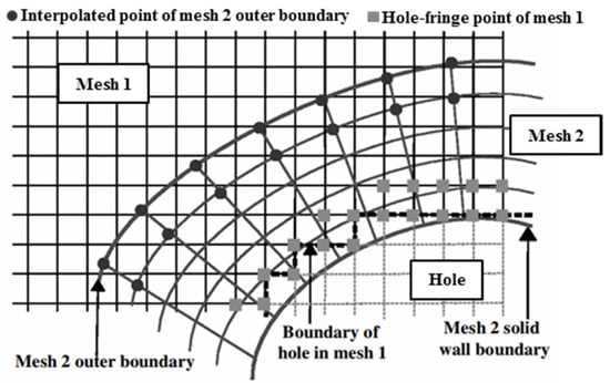
Figure 2.
Details of the overset mesh.
Three steps are required for the overset approach: hole cutting, the identification of interpolation points, and the identification of donor cells. The purpose of hole cutting is to remove unnecessary cells before calculation. The cutting face will be set in the area which needs to be removed, and then the grid points that fall into cutting face will be identified and discarded in the CFD computation process. The hole mapping method is employed for the hole-cutting process. The interpolation point identification identifies two types of interpolation points, as illustrated in Figure 2: hole-fringe points and outer boundary points. The hole-fringe points, as any point near a hole point, are easily identified. The outer-boundary point is any point that lies on the boundary of a computational mesh. The donor cells identification identifies the hexahedral donor cells with the interpolation points as the vertex. The simplest and most reliable way to find donor cells is to traverse the entire mesh domain until the correct cells are found. However, the efficiency of this method is the lowest and the use of an excellent data structure can improve the seeking speed. The attribute distributed tree (ADT) approach is employed for the donor search process.
3. Problem Setup
3.1. HUST-Ship Solver
Based on solving the dimensionless conservation equations of mass and momentum, HUST-Ship adopted the SST k-ω turbulence model to simulate the turbulent flow and multibody and multi-coordinates were employed to solve the 6DOF motion of ships. The structured overset grid technology was used for grid discretization, coupled with the single-phase level-set method to capture the change of the free surface. As a mature CFD solver applicable in the domain of ship hydrodynamics, much previous work has proved the ability of HUST-Ship [31,32].
The whole workflow is shown in Figure 3.
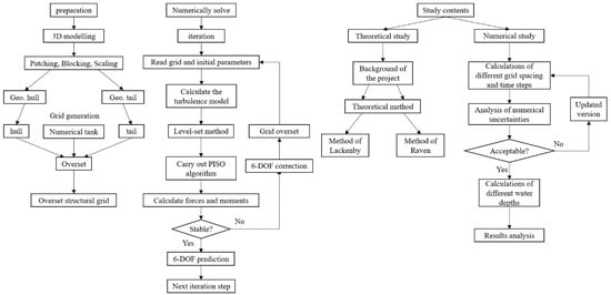
Figure 3.
The workflow flowchart.
3.2. Ship Geometry
The principle parameters of the KCS are given in Table 1.

Table 1.
Main parameters of ship geometry.
3.3. Computational Domain and Boundary Conditions
The prismatic rectangular computational domain was generated to simulate the flow around the KCS. For full-scale calculations, a larger Reynolds number resulted in the need of thinner boundary layers, which increased the number of mesh cells. Due to the symmetry of the ship geometry and the 2DOF ship motion, the hydrodynamic characteristics of the ship obtained by half of the computational domain and the whole computational domain are the same, so only half of the ship and domain were used for full-scale calculations to reduce the number of mesh cells.
Figure 4 and Figure 5 show the computational domains and the boundary conditions of the model scale and full scale respectively. The upstream is the “Inlet” boundary condition and the downstream is the “Exit” boundary condition; the Y = 0 plane of full-scale calculations is set as the symmetrical plane boundary condition “X-axis symmetry”; the side of the tank is set as a constant velocity boundary condition “Zero gradient”; the top of the domain is a far-field boundary condition “Farfield#2”; for limited water depths, the bottom of computational domains are set as the impermeable boundary “Impermeable slip, no force”, on which the force will not be calculated by the solver, while it is usually set as a “Farfield#1” boundary condition in deep water simulations.
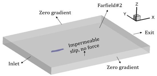
Figure 4.
The computational domain for the model-scale calculations.
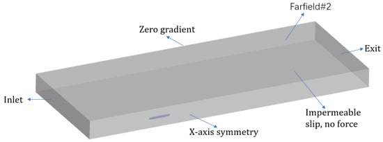
Figure 5.
The computational domain for the full-scale calculations.
Table 2 shows the mathematical description of the boundary conditions listed above.
Table 2.
The mathematical description of boundary conditions.
To simulate the different water depths of the towing tank, computational domains of different sizes are established. Since only the effect of water depth is of concern in this study, i.e., the effect of the tank wall should be ignored, so a series of computational domains that are of sufficient length and width are used. Table 3 shows the size of the full-scale computational domains.
Table 3.
The CFD computational domain size of the full-scale (half hull).
Table 4 shows the size of the model-scale domains.
Table 4.
The CFD computational domain size of the model-scale (full hull).
Figure 6 and Figure 7 give the grid of hull surface and the distribution of the overset grid of the whole computational domain respectively. Figure 8 shows the transverse and longitudinal mesh sections of the overset domain near the hull respectively.
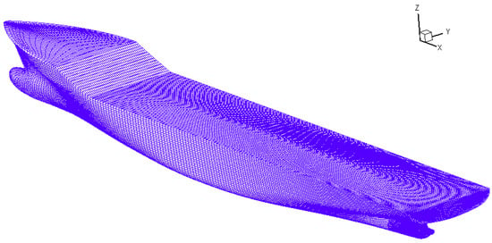
Figure 6.
The grid of the hull surface.
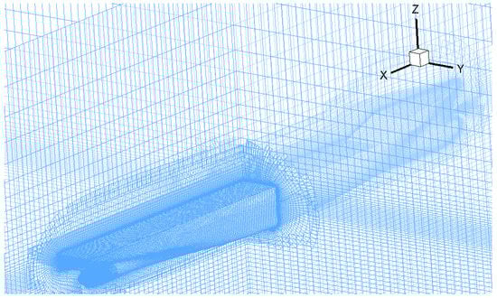
Figure 7.
The overset grid of the computational domain.
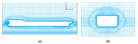
Figure 8.
2D mesh sections: (a) midsection in the Y = 0 plane and (b) midsection in the X = 0.5LPP plane.
3.4. Estimation of Numerical Uncertainties
Verification and validation of the numerical method for calculations of the bare hull resistance have been carried out. ITTC V & V (Verification and Validation) 2008 [34] A validation procedure was used to estimate the uncertainties of the numerical method.
In general, the numerical uncertainty includes the following aspects: uncertainty of iteration steps , the uncertainty of the grid space , the uncertainty of the time step and the other parameters uncertainty . For URANS solver HUST-Ship, , and could be ignored utilizing lots of iterations. For the specific computation in this study, and are of the most concern. Therefore, the numerical uncertainty can be expressed as follows:
Systematic grid-spacing and time-step studies were carried out using the generalized Richardson extrapolation method according to the literature [35].
At first, the uniform parameter refinement ratio between solutions is assumed as:
in which , , and are the space of the coarse grid, medium grid, and fine grid or time step, respectively. , , and are the calculation results obtained by fine, medium and coarse grid spacing or time step, respectively. and are the differences between solutions of medium-fine and coarse-medium grid spacings, respectively. The convergence ratio R is defined as:
There are three possible conditions:
- Monotonic convergence (MC):
- Oscillatory convergence (OC):
- Divergence (D):
When monotonic convergence is achieved, the Richardson extrapolation method can be used. The estimated numerical error and order of accuracy can be calculated as:
The correction factor is defined as:
where is an estimated value for the limiting order of accuracy as the spacing size goes to zero; generally, . The numerical error , benchmark result and uncertainty can be estimated from:
When is significantly less than or greater than 1, which means the solutions are far away from the asymptotic range, the numerical uncertainty can be calculated from:
4. Results
The directions of the drag force, trim angle, and sinkage are defined as shown in Figure 9.
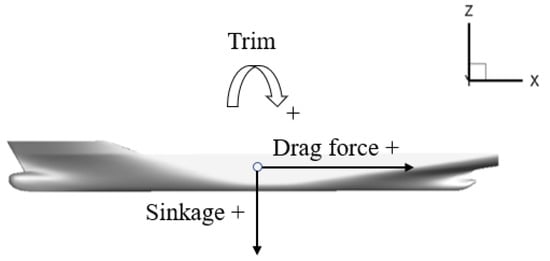
Figure 9.
The directions of the drag force, trim angle and sinkage.
4.1. Verification and Validation
To ensure the reliability of numerical simulation, verification and validation study is conducted for the model-scale ship and the full-scale ship, in deep-water condition.
4.1.1. Model Scale (Fr = 0.26, Re = 1.477e+7)
In the previous work [32], the sensitivity of grid spacing and time step was studied for a KCS scaled model. The velocity of the scaled model is 2.197 m/s and the length between perpendiculars is 7.2786. Three grid cases and three time-step schemes were conducted for the KCS scaled model, as a preparation step; it is a key step to ensure the accuracy of the results. Table 5 shows the results obtained by the different grid cases and Table 6 shows the results obtained for different time step cases. Table 7 shows the results of numerical uncertainty of the KCS scaled model. Three different grids were generated with a grid refinement ratio and three time-step schemes were generated with a refinement ratio of 2.
Table 5.
Total resistance coefficients of different grid cases of the 1:31.6 scaled model.
Table 6.
The total resistance coefficients of different time steps of the 1:31.6 scaled model.
Table 7.
The numerical uncertainties of resistance of the 1:31.6 scaled model.
For both grid-spacing and time-step, the convergence factor R was between 0 and 1, which meant that monotonic convergence was achieved and the generalized Richardson extrapolation method could be used. From Table 7, it can be observed that the uncertainties of the grid and time-step for the total resistance coefficient of the 1:31.6 scaled model were 1.984% and 0.025%, respectively, where is the bench mark experimental data obtained from Equation (25) and the total numerical uncertainty is 1.984% .
4.1.2. Full Scale (Fr = 0.26, Re = 2.84e+9)
Three grid cases and three time-step schemes were conducted for the full-scale KCS ship. Table 8 shows the results obtained for different grid cases and Table 9 shows the results obtained for different time step cases. Table 10 shows the results of numerical uncertainty. Three different grids were generated with a constant refinement ratio and three time-step schemes were generated with a constant refinement ratio . The reference EFD value comes from the literature [29].
Table 8.
The total resistance coefficients of different grids of the full-scale KCS.
Table 9.
The total resistance coefficients of the different time steps of the full-scale KCS.
Table 10.
The numerical uncertainties of the total resistance coefficients of the full-scale KCS.
For both grid-spacing and time-step, the convergence factor R was between 0 and 1, which meant that monotonic convergence was achieved and the generalized Richardson extrapolation method could be used. From Table 10, it can be observed that the uncertainties of grid and time-step for the total resistance coefficient of the 1:31.6 scaled model were 4.926% and 0.924%, respectively, where is the bench mark experimental data obtained from Equation (25) and the total numerical uncertainty is 5.012%.
4.1.3. Grid Spacing Sensitivity
For ships passing through the shallow-water channels, the flow parameters under the keel can change significantly, so the grid spacing between the bottom of the tank and the keel may significantly affect the calculation results.
As a reference for subsequent calculations, the grid spacing of the model scaled at H/T = 4 is chosen to study. Table 11 and Table 12 show the results of the convergence study.
Table 11.
The grid spacing convergence analysis.
Table 12.
The numerical uncertainties of the grid spacing under the keel.
Since the calculated resistance coefficients of the middle and fine grid spacing are very close, the subsequent calculations are carried out using the middle spacing to ensure accuracy and to reduce the number of grid cells for computation processing.
4.1.4. Validation Based on EFD data
Assuming that the benchmark experimental value is D, the comparison error E can be defined as:
in which, is the benchmark numerical result from Equation (25).
The validation uncertainty is given by:
Where, is the uncertainty of the experimental data provided for the KCS towed resistance. The results of the validation study are given in Table 13.
Table 13.
Validation study.
4.2. Force and Attitude
4.2.1. Model Scale (Fr = 0.26, Re = 1.26e + 7)
The velocity of the scaled model is 2.197 m/s and the length between perpendiculars is 7.2786 m, which are same as presented with the previous cases of uncertainty analysis. The only difference is that the experimental kinematic viscosity leads to a slightly different Reynolds number from previous studies, however, previous studies can still be used to prove that the selected grid and time step are appropriate. As shown in Figure 10 and Table 14, the total resistance coefficient increases with a decrease of water depth; the increase of ship resistance in shallow water is shown intuitively. With the decrease of water depth, the total resistance coefficient increases gradually, but the total resistance coefficient of the three calculation cases with draft ratios H/T = 6, H/T = 8, and H/T = 10 does not increase significantly compared with the deep-water resistance measured in the model test. According to the International Towing Tank Conference (ITTC), the water depth H which can ignore the shallow water effect shall meet the following requirements:
where B is the maximum width of the ship; T is the draft; V is the ship speed; and g is the acceleration of gravity.
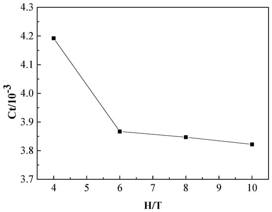
Figure 10.
The total resistance coefficients of the KCS scaled model with different depth/draft ratios (H/T).
Table 14.
The results of resistance, sinkage and trim.
A further calculation shows that the calculation cases of H/T = 6, H/T = 8, and H/T = 10 are in this range, which indicates that the shallow-water effect is not so obvious.
Table 14 shows the detailed data of the resistance coefficients, sinkage, and trim in different calculation cases. The experimental fluid dynamics (EFD) value is obtained from the Tokyo 2015 workshop website.
As shown in Figure 11, the sinkage of the KCS increases monotonically with the decrease of H/T. There are many empirical formulas for predicting sinkage and the calculation results were compared with Raven’s method in the following section. Figure 12 shows the changing trend of the trim angle in different water depths; the negative value means trim by the bow. As the H/T decreases, the trim angle gradually becomes larger.
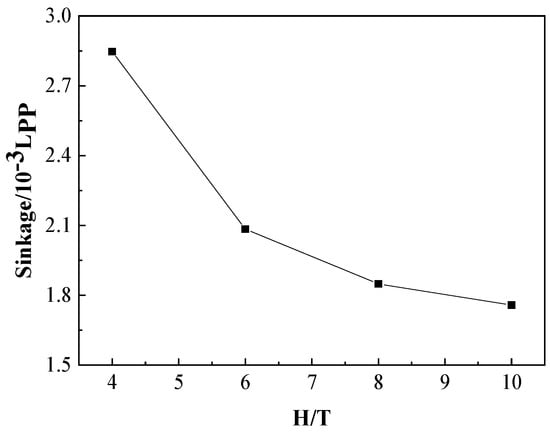
Figure 11.
The dimensionless sinkage of the KCS scaled model with different depth/draft ratios (H/T).
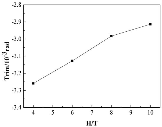
Figure 12.
The trim angle with different depth/draft ratios of KCS scaled model (H/T).
4.2.2. Full Scale (Fr = 0.26, Re = 2.84e + 9)
As shown in Figure 13, the total resistance coefficient increases with the decrease of water depth; the increase of ship resistance in shallow water is shown intuitively. For a KCS, with the decrease of water depth, the total resistance coefficient increases gradually, but the total resistance coefficient of the two working conditions with draft ratio H/T = 6.7 and H/T = 10 does not increase significantly compared with the deep-water working condition (H/T = 21.3), for which the water depth is equal to the length between perpendiculars of the KCS.
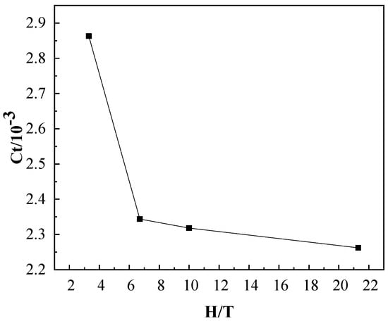
Figure 13.
Total resistance coefficients of the full-scale KCS with different depth/draft ratios (H/T).
4.2.3. Comparison with the Existing Experimental Results
Some calculations were conducted for a 1:75 KCS scaled model to compare with the experimental study of Khaled Elsherbiny [36]; a low-speed point (FnH = 0.32) and a high-speed point (FnH = 0.8) are chosen for comparison. The comparison results of the total resistance coefficient and sinkage are given in Table 15. The EFD value is obtained from the results in the literature by interpolation.
Table 15.
The comparison with the experimental value.
4.3. Wave Properties
As we know, the dispersion relation for limited water depth is:
or
Evidently, for a larger λ/h, the factor introduces a dependence on the ratio of wavelength to water depth. When the water depth h further decreases and the ratio λ/h becomes large, as Equation (27) shows, the propagation speed of waves will reach a limiting value of This indicates that there is an upper limit to the wave propagation speed in shallow water.
The different propagation speeds of waves in different water depths led to the differences in wave properties among the calculation cases. To show the wave properties, the nondimensionalized wave height on the hull surface and the Y = 0.1509 Lpp section are extracted.
4.3.1. Model Scale
As shown in Figure 14, the wave height curves for the cases of H/T = 6, H/T = 8, and H/T = 10 almost coincide, while for the H/T = 4 case, there is a clear departure from the other curves. It can also be seen that the wave height distribution characteristics on the Y = 0.1509 Lpp section are very similar to those on the hull surface, but tend to be flat on the whole. The further away from the ship, the more horizontal the free surface becomes, because the kinetic energy of the wave gradually changes into potential energy in the process of propagation.
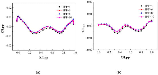
Figure 14.
The model-scale wave profiles at different water depths: (a) on the hull surface and (b) on the Y = 0.1509 Lpp section.
4.3.2. Full Scale
It can be seen from Figure 15 that the wave height distribution characteristics of the full-scale ship are very similar to the wave properties of the scaled model.
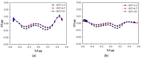
Figure 15.
The full-scale wave profiles at different water depths: (a) on the hull surface and (b) on the Y = 0.1509 Lpp section.
4.4. Comparison with the Method of Raven
To get a proportion of viscous resistance, the estimation method of the form factor is introduced in this study.
According to the literature, “the most popular empirical formula for determining the form factor is attributed to Watanabe” [37].
The calculated value of KCS is close to 0.1.
4.4.1. Correction Process
After studying the effect of shallow water on viscous resistance, Raven began to do further research on the shallow water effect. A complete set of shallow water resistance correction procedures was proposed in his paper [38]. The correction steps are following as:
- The correction of the viscous resistance coefficient isin which T represents the draft; H represents the water depth; and represents the ratio of shallow-water viscous resistance coefficient to deep-water viscous resistance coefficient.
- No correction of wave resistance in the range of the critical Froude number .After analyzing many numerical results and a large amount of test data, Raven thought that the change of wave resistance could be ignored when the Froude depth number is under the critical value 0.65 in Raven’s study.
- Estimate additional sinkageA good prediction formula was first proposed in the 1960s [39]; then Hooft [11] made a small change on it. The estimation formula of additional sinkage is derived from the formula proposed by Hooft; Ankudinov’s [40] idea was used by Raven for reference in the process.in which L is the ship length, is the displacement volume; and is the Froude depth number.
- Estimate the resistance increase due to additional sinkagein which is the factor that represents the effect of the sinkage increase caused by shallow water and is the additional displacement volume due to additional sinkage.
- The total resistance coefficient increase factor caused by shallow water isin which is the correction factor of total resistance; is the relative contribution of viscous resistance in deep water at the same ship speed with a computational case; and , which restricts the use of this method to the case where .
- Range of applicability
- the Froude depth number should be less than 0.65. Otherwise, a significant increase of wave-making resistance will occur.
- the ratio of the draft to the water depth T/H should be less than 0.5. For a higher value, the viscous resistance could not be accurately estimated using a simple formula.
- , the increase of displacement volume should be no more than 5%, otherwise, a better method may be needed to estimate the effect of the draft difference.
4.4.2. Model Scale
Table 16 gives the brief process of resistance correction using Raven’s method and compares the results with CFD results; a maximum difference of 5.8771% appears when H/T = 4.
Table 16.
The difference of total resistance coefficients between Raven’s method and CFD results.
As shown in Figure 16, the calculation results show quite good agreement with Raven’s method when the water depths are deeper, but as the Froude depth number becomes larger with the decreasing of water depth h, a larger difference between the estimation and calculation occurs. In the case of the shallowest water depth, there is a maximum difference, and we find the Froude number, in this case, is close to the critical value 0.65. In Raven’s correction method, the increase of wave resistance was ignored when FnH < 0.65, however, a significant increase in wave resistance may occur when FnH > 0.65, which could be the reason why a small difference is observed.
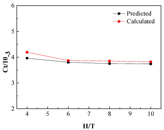
Figure 16.
The comparison of the model-scale total resistance coefficients, estimated from Raven’s equations (Black) and computed by CFD code (Red).
As can be seen in Figure 17, a clear difference appears in the case of H/T = 4: we cannot make sure here whether it is caused by a deficiency of the CFD simulation or a deficiency of the empirical formula. However, when considering the resistance increase caused by an additional sinkage, Raven adopted the method of constant admiralty coefficient, which can be defined as:
in which, and , and are the displacement and effective power at different water depths. As we know, the effective power can be expressed as a product of resistance and ship speed, i.e., . As a result, the ratio of ship resistance at the same speed in different water depths can be derived as:
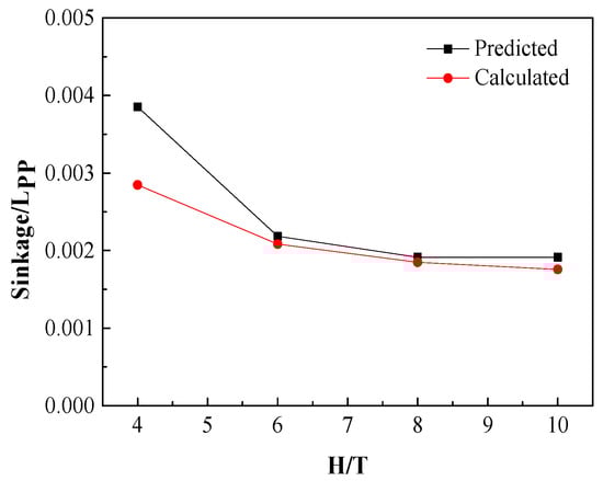
Figure 17.
The comparison of model-scale dimensionless sinkage between the predicted value obtained by Raven’s formula (Black) and the calculated value obtained by CFD simulations (Red).
Assumed is the resistance at a finite water depth and is the resistance in unrestricted water, Equation (31) can be derived.
Although the difference between the predicted sinkage and the value calculated by the CFD code is up to 26%, the value can as low as 0.5% when comparing the , which means it has little influence on estimating the increase of total resistance.
4.4.3. Full Scale
Table 17 gives the brief process of resistance correction using the Raven method and compares the results with the CFD results; a maximum difference of 20.942% appears when H/T = 3.3.
Table 17.
The difference of total resistance coefficients between Raven’s method and CFD results.
As shown in Table 11, the difference between the CFD results and the prediction results are within the acceptable range at the water depth to draft ratios H/T = 6.7 and H/T = 10, but an unacceptable difference occurs when H/T = 3.3.
Even though the comparison differences between the CFD results and the prediction results are larger than the model-scale comparison differences, a similar trend is observed: the largest difference occurs in the case of the minimum water depth to draft ratio. Actually, with the increase of the Froude depth number, the increase of wave resistance in shallow water may be significant, however, it was ignored in the process of resistance correction, which may cause an underestimate of the total resistance coefficient. In addition, there is no experimental data of full-scale trials, so the reference value is extrapolated using the value measured in model test, which may further increase the differences between the CFD and prediction results.
5. Discussion
5.1. Shallow-Water Effect on Ship Resistance
5.1.1. Viscous Resistance
According to fluid dynamics, when encountering a channel of limited water depth, the flow velocity between the tank bottom and the ship keel will increase significantly. As a result, the static pressure of particles will decrease, which results in the dynamic sinkage of ships, as well as the increase of frictional resistance. In addition, the increase of the relative velocity between the ship and the water results in an increase of the pressure gradient, which increases the viscous pressure resistance.
Figure 18 shows the model-scale dimensionless flow velocity in the x-axis direction between the ship keel and the tank bottom. The number marked on the figure represents the overspeed ratio γ, which is defined as:
where U represents the dimensionless flow velocity in the x-axis, and is the nondimensionalized ship speed, i.e., = 1. As a result, can be derived.
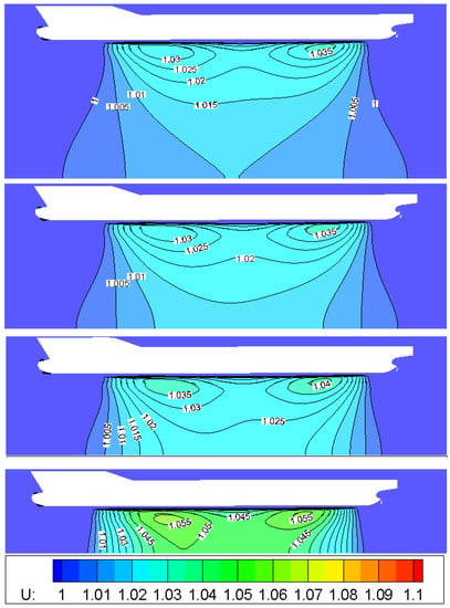
Figure 18.
The overspeed ratios at different water depths for the 1:31.6 scaled model of the KCS (water depth decreases from top to bottom, corresponding to H = 4T, H = 6T, H = 8T, H = 10T respectively).
It is evident from the figure that both the peak value of the overspeed ratio and the gradient of flow velocity increases with a decrease of water depth, which is in line with the above analysis.
5.1.2. Wave Resistance
The influence factor of wave resistance is the Froude depth number FnH. The critical value of the Froude depth number is FnH = 1, where FnH < 1 represents the interval of subcritical speed, and FnH > 1 corresponds to the interval of supercritical speed.
According to the wave theory, the wave resistance increases significantly with the increase of the Froude depth number in the subcritical interval. However, the wave resistance decreases abnormally with the increase of FnH after the ship speed exceeds the critical value.
Figure 19 shows the wave patterns of the full-scale simulations. It can be seen from the figure that a higher Froude depth number indicates a higher wave height contour density. It also means that a higher Froude depth number indicates a larger wave resistance.
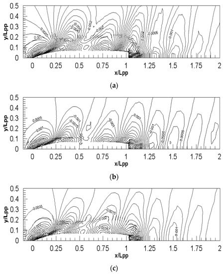
Figure 19.
The wave patterns of full-scale simulations for different Froude depth numbers: (a) FnH = 0.66, (b) FnH = 0.47 and (c) FnH = 0.38.
6. Conclusions
Taking the full-scale and model-scale KCS as study objects, numerical simulations were conducted to calculate the ship resistance at different water depth/draft ratios. The hydrodynamic force, sinkage, trim angle, and wave properties at different water depths are presented and discussed. The in-house URANS CFD solver, based on the finite difference method (FDM), is used for this study. Two right-handed Cartesian coordinate systems are established to predict the 2-DOF motion of the forward ship and the single-phase level-set method is used to capture the change of the free surface. Lots of previous applications of HUST-Ship show quite a good accuracy. All results of resistance, trim angle, sinkage, and wave patterns show differences among different water depths, which indicates that the HUST-Ship solver can well express the effect of shallow water.
Verification study in terms of grid and time step sensitivity was performed to make sure that the numerical method was reliable; the Richardson extrapolation method was used in the process. A validation study was then conducted to judge the availability of the numerical results. Furthermore, the sensitivity of the grid spacing between the keel and the bottom of the towing tank was studied to obtain a proper grid spacing of the computational domain.
The results of total resistance coefficients and dynamic sinkage obtained by the CFD simulations were compared with the predicted value obtained by Raven’s method. The comparison indicates that the differences between the CFD results and Raven’s estimation results are extremely small in larger water depths. When the water depth becomes shallower, the differences between CFD and Raven’s estimation increased rapidly. As Raven claimed in his paper, the increase of wave resistance can be ignored when , however, some classical literatures support different critical values. As the results of this paper show, a lower critical value of FnH may be more appropriate, since the difference between the estimation and the CFD goes up to 20% when FnH is over 0.65 (0.66) in the full-scale simulation, and a maximum difference of 5.8771% occurs in the model-scale simulation when the FnH is close to 0.65 (0.61). Comparing the model-scale simulation results with the full-scale simulation results, a similar trend for the change of resistance and altitude with a decrease of water depths is evident.
Even though the conclusion can be roughly obtained, the drawback of this paper is that only the designed speed of the KCS is considered, and the important impact index FnH can only be controlled by changing the water depth. Future works will contain the simulation of different Froude numbers to get a more persuasive conclusion.
Author Contributions
D.F.: methodology, investigation, resources, writing–original draft, funding acquisition. B.Y.*: software, data curation, visualization, validation, formal analysis. Z.Z.: writing–review and editing, Project administration, funding acquisition. X.W.: supervision, funding acquisition. All authors have read and agreed to the published version of the manuscript.
Funding
This research received no external funding.
Acknowledgments
The research work comes from the ITTC workshop in 2019. This research was sponsored by the Advanced Research Common Technology Project of CHINA CMC (41407010401, 41407020502). The essential support is greatly acknowledged.
Conflicts of Interest
The authors declare no conflict of interest.
List of Symbols
| Direction of the independent coordinates | |
| Ship service speed, incoming velocity | |
| Length between perpendiculars | |
| ρ | Density of water |
| Kinematic viscosity | |
| H | Water depth |
| T | Draft of the ship |
| Froude depth number | |
| Dynamic pressure coefficient | |
| Reynolds stress | |
| k | Turbulent kinetic energy |
| ,, | Components of moment of inertia with respect to the gravity center |
| X, Y, Z | Components of external forces acting on the hull |
| K, M, N | Components of external moments acting on the hull |
| Distance from any point in the flow field to the free surface | |
| Time step | |
| EFD | Results obtained by experimental fluid dynamics |
| MC | Monotonic convergence |
References
- Sezen, S.; Cakici, F. Numerical prediction of total resistance using full similarity technique. China Ocean. Eng. 2019, 33(4), 493–502. [Google Scholar] [CrossRef]
- Zeng, Q.; Hekkenberg, R.; Thill, C.; Rotteveel, E. A numerical and experimental study of resistance, trim and sinkage of an inland ship model in extremely shallow water. In Proceedings of the International Conference on Computer Applications in Shipbuilding, Singapore, 26–28 September 2017; pp. 26–28. [Google Scholar]
- Raven, H.C. A computational study of shallow-water effects on ship viscous resistance. In Proceedings of the 29th Symposium on Naval Hydrodynamics, Gothenburg, Sweden, 27 August 2012. [Google Scholar]
- Choi, J.; Min, K.-S.; Kim, J.; Lee, S.; Seo, H. Resistance and propulsion characteristics of various commercial ships based on CFD results. Ocean. Eng. 2010, 37, 549–566. [Google Scholar] [CrossRef]
- Tezdogan, T.; Demirel, Y.K.; Kellett, P.; Khorasanchi, M.; Incecik, A.; Turan, O. Full-scale unsteady RANS CFD simulations of ship behaviour and performance in head seas due to slow steaming. Ocean. Eng. 2015, 97, 186–206. [Google Scholar] [CrossRef]
- Yang, D.; Sun, Z.; Jiang, Y.; Gao, Z. A Study on the Air Cavity under a Stepped Planing Hull. J. Mar. Sci. Eng. 2019, 7, 468. [Google Scholar] [CrossRef]
- Cucinotta, F.; Guglielmino, E.; Sfravara, F.; Strasser, C. Numerical and experimental investigation of a planing Air Cavity Ship and its air layer evolution. Ocean. Eng. 2018, 152, 130–144. [Google Scholar] [CrossRef]
- Cucinotta, F.; Guglielmino, E.; Sfravara, F. A critical CAE analysis of the bottom shape of a multi stepped air cavity planing hull. Appl. Ocean. Res. 2019, 82, 130–142. [Google Scholar] [CrossRef]
- Duy, T.-N.; Hino, T.; Suzuki, K. Numerical study on stern flow fields of ship hulls with different transom configurations. Ocean. Eng. 2017, 129, 401–414. [Google Scholar] [CrossRef]
- Jachowski, J. Assessment of ship squat in shallow water using CFD. Arch. Civ. Mech. Eng. 2008, 8, 27–36. [Google Scholar] [CrossRef]
- Hooft, J.P. The Influence of Nautical Requirements on the Dimensions and Layout of Entrance Channels and Harbours; Proc. International Course Modern Dredging: The Hague, The Netherlands, 1977. [Google Scholar]
- Pacuraru, F.; Domnişoru, L. Numerical investigation of shallow water effect on a barge ship resistance. IOP Conf. Series Mater. Sci. Eng. 2017, 227, 012088. [Google Scholar] [CrossRef]
- Ji, S.; Ouahsine, A.; Smaoui, H.; Sergent, P. 3D Numerical Modeling of Sediment Resuspension Induced by the Compounding Effects of Ship-Generated Waves and the Ship Propeller. J. Eng. Mech. 2014, 140, 04014034. [Google Scholar] [CrossRef]
- Linde, F.; Ouahsine, A.; Huybrechts, N.; Sergent, P. Three-Dimensional Numerical Simulation of Ship Resistance in Restricted Waterways: Effect of Ship Sinkage and Channel Restriction. J. Waterw. Port. Coastal. Ocean. Eng. 2017, 143, 06016003. [Google Scholar] [CrossRef]
- Du, P.; Ouahsine, A.; Sergent, P.; Hu, H. Resistance and wave characterizations of inland vessels in the fully-confined waterway. Ocean. Eng. 2020, 210, 107580. [Google Scholar] [CrossRef]
- Liu, Y.; Zou, Z.; Zou, L.; Fan, S. CFD-based numerical simulation of pure sway tests in shallow water towing tank. Ocean. Eng. 2019, 189, 106311. [Google Scholar] [CrossRef]
- Xu, H.; Hinostroza, M.; Wang, Z.; Soares, C.G. Experimental investigation of shallow water effect on vessel steering model using system identification method. Ocean. Eng. 2020, 199, 106940. [Google Scholar] [CrossRef]
- Tang, X.; Tong, S.; Huang, G.; Xu, G. Numerical investigation of the maneuverability of ships advancing in the non-uniform flow and shallow water areas. Ocean. Eng. 2020, 195, 106679. [Google Scholar] [CrossRef]
- Schlichting, O. Schiffwiderstand auf beschränkter wassertiefe: Widerstand von seeschiffen auf flachem wasser. Jahrbuch der Schiffbautechnischen Gesellschaft; Springer: Hanburg, Germany, 1934; Volume 35, p. 127. [Google Scholar]
- Lackenby, H. The Effect of Shallow Water on Ship Speed. Nav. Eng. J. 1964, 76, 21–26. [Google Scholar]
- ITTC. Speed and Power Trials, Part 2, Analysis of Speed/Power Trial Data. In Proceedings of the 25th ITTC, Copenhagen, Denmark; 2014. Available online: https://ittc.info/media/4210/75-04-01-012.pdf (accessed on 21 January 2020).
- Jiang, T. A New Method for Resistance and Propulsion Prediction of Ship Performance in Shallow Water; Elsevier: Amsterdam, The Netherlands, 2001; pp. 509–515. [Google Scholar]
- Raven, H.C. A new correction procedure for shallow-water effects in ship speed trials. In Proceedings of the 13th International Symposium on Practical Design of Ships and Other Floating Structures, Copenhagen, Denmark, 4–8 September 2016. [Google Scholar]
- ITTC. Procedures and Guidelines. In Proceedings of the 28th ITTC, Wuxi, China; 2017. [Google Scholar]
- Guo, L.; Yu, J.; Chen, J.; Jiang, K.; Feng, D. Unsteady Viscous CFD Simulations of KCS Behaviour and Performance in Head Seas. In International Conference on Offshore Mechanics and Arctic Engineering; American Society of Mechanical Engineers: New York, NY, USA, 2018; Volume 51210, p. V002T08A040. [Google Scholar] [CrossRef]
- Carrica, P.M.; Wilson, R.V.; Noack, R.W.; Stern, F. Ship motions using single-phase level set with dynamic overset grids. Comput. Fluids 2007, 36, 1415–1433. [Google Scholar] [CrossRef]
- Ji, S.C.; Ouahsine, A.; Smaoui, H.; Sergent, P. 3-D Numerical Simulation of Convoy-Generated Waves in a Restricted Waterway. J. Hydrodyn. 2012, 24, 420–429. [Google Scholar] [CrossRef]
- Burg, C.O.E. Single-phase level set simulations for unstructured incompressible flows. In Proceedings of the 17th AIAA Computational Fluid Dynamics Conference, Toronto, ON, Canada, 6–9 June 2005. [Google Scholar]
- Castro, A.M.; Carrica, P.M.; Stern, F. Full scale self-propulsion computations using discretized propeller for the KRISO container ship KCS. Comput. Fluids 2011, 51, 35–47. [Google Scholar] [CrossRef]
- Hu, K. Near-Wall Treatment. Available online: http://url.cn/jbbb6MO5 (accessed on 20 January 2020).
- Wang, X.; Liu, L.; Zhang, Z.; Feng, D. Numerical study of the stern flap effect on catamaran’ seakeeping characteristic in regular head waves. Ocean. Eng. 2020, 206, 107172. [Google Scholar] [CrossRef]
- Feng, D.; Yu, J.; He, R.; Zhang, Z.; Wang, X. Free running computations of KCS with different propulsion models. Ocean. Eng. 2020, 214, 107563. [Google Scholar] [CrossRef]
- Tokyo 2015 CFD Workshop. Available online: https://t2015.nmri.go.jp/ (accessed on 15 January 2020).
- ITTC, Uncertainty Analysis in CFD, Part 1, Verification and Validation Methodology and Procedures. In Proceedings of the 25th ITTC, Fukuoka, Japan, 14–20 September 2008; Available online: https://ittc.info/media/4184/75-03-01-01.pdf (accessed on 22 January 2020).
- Stern, F.; Wilson, R.V.; Coleman, H.W.; Paterson, E.G. Comprehensive Approach to Verification and Validation of CFD SimulationsMethodology and Procedures. J. Fluids Eng. 2001, 123, 793–802. [Google Scholar] [CrossRef]
- Elsherbiny, K.; Tezdogan, T.; Kotb, M.; Incecik, A.; Day, S. Experimental analysis of the squat of ships advancing through the New Suez Canal. Ocean. Eng. 2019, 178, 331–344. [Google Scholar] [CrossRef]
- Larsson, L.; Raven, H.C. Ship Resistance and Flow; The Society of Naval Architects and Marine Engineers: Jersey City, NJ, USA, 2010; p. 103. [Google Scholar]
- Raven, H.C. A method to correct shallow-water model tests for tank wall effects. J. Mar. Sci. Technol. 2018, 24, 437–453. [Google Scholar] [CrossRef]
- Tuck, E.O. Shallow-water flows past slender bodies. J. Fluid Mech. 1966, 26, 81. [Google Scholar] [CrossRef]
- Ankudinov, V.; Daggett, L.; Huval, C.; Hewlett, C. Squat predictions for maneuvering applications. In Proceedings of the International Conference on Marine Simulation and Ship Maneuverability MARSIM’96, Copenhagen, Denmark, 9–13 September 1996; pp. 467–495. [Google Scholar]


© 2020 by the authors. Licensee MDPI, Basel, Switzerland. This article is an open access article distributed under the terms and conditions of the Creative Commons Attribution (CC BY) license (http://creativecommons.org/licenses/by/4.0/).